On the Global Dynamics of the Anisotropic Manev Problem

Abstract

We study the global flow of the anisotropic Manev problem, which describes the planar motion of two bodies under the influence of an anisotropic Newtonian potential with a relativistic correction term. We first find all the heteroclinic orbits between equilibrium solutions. Then we generalize the Poincaré-Melnikov method and use it to prove the existence of infinitely many transversal homoclinic orbits. Invoking a variational principle and the symmetries of the system, we finally detect infinitely many classes of periodic solutions.

1 Introduction

The anisotropic Manev problem describes the motion of two point masses in an anisotropic configuration plane under the influence of a Newtonian force-law with a relativistic correction term. The isotropic case is the classical Manev problem; its origins lie in the work of Newton, who introduced it in Principia aiming to understand the apsidal motion of the moon (see [11, 14]). Manev found in the 1930s that a proper choice of the constants that show up in the correction term allow the theoretical explanation of the perihelion advance of Mercury and of the other inner planets.

The first author suggested the study of the anisotropic Manev problem in 1995, hoping to find connections between classical, quantum, and relativistic mechanics. It was indeed proved in [10] that the rich collision-orbit manifold of the system exhibits classical, quantum, and relativistic properties. This encouraged further studies, as for example [15] and [24]. In [15], using a suitable generalization of the Poincaré-Melnikov method (see [4, 17, 21, 28] for the classical approach or [5, 6] for a parallel, at least in part, complementary approach), we proved that chaos occurs on the zero-energy manifold, thus showing the complexity of the dynamics. Using perturbations techniques and the Poincaré continuation method, the second author investigated in [24] the classes of periodic solutions that arise from symmetries in the case of small values of the anisotropy parameter.

In this paper we gain a better understanding of the complicated global dynamics encountered in this problem. We first prove that negative-energy solutions are bounded and find the heteroclinic orbits that connect the equilibria of the collision manifold, which we obtain through McGehee-type transformations (see [20]). Physically they correspond to ejection-collision orbits. Then we employ perturbation techniques to detect possible global chaotic behaviour. As remarked in [24], the perturbation analysis of [15, 24] cannot be used to study ejection-collision solutions. However, we surpass this difficulty with the help of McGehee-type coordinates, which allow us to view the anisotropic Manev problem as a perturbation of the classical Manev case.

Using an approach inspired by [5, 6], which works in some degenerate cases—as for example those of unstable nonhyperbolic points or critical points located at infinity (see [7, 8, 9, 15]), we develop a suitable extension of the Poincaré-Melnikov method, which we use to prove the existence of transversal homoclinic orbits to a periodic one. It is interesting to note that our result extends the one obtained in [7, 8, 9] to a non-Hamiltonian system that has negatively and positively asymptotic sets to a nonhyperbolic periodic orbit. In the present context the asymptotic sets are the stable and the unstable manifolds.

Then we return to the original coordinates and apply a variational principle for detecting periodic orbits. Using the rotation index, we divide the set of periodic paths into homotopy classes, which are Sobolev spaces. Then we use the lower semicontinuity version of Hilbert’s direct method (due to Tonelli, see [26]) to find a minimizer of the action in each class. According to the least action principle, the minimizer is a solution of the anisotropic Manev problem. We prove that the minimizer exists, belongs to the homotopy class, and is a solution in the classical sense. This generalizes a result obtained by the second author, [24], where it was shown that such orbits exist for small values of $\mu>1$. In the end we put into the evidence some new properties of symmetric periodic orbits.

The idea of using variational principles to obtain periodic orbits for $n$-body-type particle systems first appeared in [23] and has been recently used in connection with symmetry conditions to obtain new periodic orbits in the classical $n$-body problem (see [2]). But unlike the Newtonian case, the Manev force is “strong” (as defined in [16]), so the variational method is easier to apply in our situation than in the Newtonian one. This is because in the Manev case we do not have to deal with the difficulty of avoiding collision orbits, which have infinite action and therefore cannot be minimizers.

Our paper is organized as follows. In Section 2 we write the equations of motion and transform them to an equivalent system using a “blow-up” technique devised by McGehee, which allow us to introduce the concept of a collision manifold. In Section 3 we present two global results: the boundedness of the solutions for negative energy and the existence of certain symmetric ejection-collision orbits. In Section 4 we describe the anisotropic Manev problem as a perturbation of the Manev case. In Section 5 we develop a suitable generalization of the Poincaré-Melnikov method and in Section 6 we apply it to find infinitely many transverse homoclinic orbits that show that the dynamics of the problem is extremely complex, possibly chaotic. Finally, in Section 7 we use a variational principle to prove the existence of infinitely many classes of symmetric periodic orbits.

2 Equations of Motion

The (planar) anisotropic Manev problem is described by the Hamiltonian

$$H={1\over 2}{\bf p}^{2}-{1\over\sqrt{x^{2}+\mu y^{2}}}-{b\over x^{2}+\mu y^{2}},$$ (1)

where $\mu>1$ is a constant, ${\bf q}=(x,y)$ is the position of one body with respect to the other considered fixed at the origin of the coordinate system, and ${\bf p}=(p_{x},p_{y})$ is the momentum of the moving particle. The constant $\mu$ measures the strength of the anisotropy and we can very well take $\mu<1$; but to remain consistent with the choice made in previous papers, we will consider $\mu>1$. For $\mu=1$ we recover the classical Manev problem. The equations of motion are

$$\left\{\begin{array}[]{l}\dot{\bf q}={\bf p}\\ \dot{\bf p}=-{\partial H\over\partial{\bf q}}.\end{array}\right.$$ (2)

The Hamiltonian provides the first integral

$$H({\bf p}(t),{\bf q}(t))=h,$$ (3)

where $h$ is a real constant. Unlike in the classical Manev case, the angular momentum $K(t)={\bf p}(t)\times{\bf q}(t)$ does not yield a first integral. This is because the anisotropy of the plane destroys the rotational invariance.

Since our first goal is to study collision and near collision solutions, it is helpful to transform system (2) using a method developed by McGehee [20]. The idea is to “blow-up” the collision singularity, replace it with a so-called collision manifold and extend the phase space to it. The collision manifold is fictitious in the sense that it has no physical meaning. However, studying the flow on it provides useful information about near-collision orbits. Consider the coordinate transformations

$$\left\{\begin{array}[]{l}r=|{\bf q}|\\ \theta=\arctan(y/x)\\ v=\dot{r}r=(xp_{x}+yp_{y})\\ u=r^{2}\dot{\theta}=(xp_{y}-yp_{x}),\end{array}\right.$$ (4)

and the rescaling of time

$$d\tau=r^{-2}dt.$$ (5)

Composing these transformations, which are analytic diffeomorphisms in their respective domains, system (2) becomes

$$\left\{\begin{array}[]{l}r^{\prime}=rv\\ v^{\prime}=2r^{2}h+r\Delta^{-1/2}\\ \theta^{\prime}=u\\ u^{\prime}=(1/2)(\mu-1)(r\Delta^{-3/2}+2b\Delta^{-2})\sin 2\theta\end{array}\right.$$ (6)

and the energy relation (3) takes the form

$$u^{2}+v^{2}-2r\Delta^{-1/2}-2b\Delta^{-1}=2r^{2}h,$$ (7)

where $\Delta=\mu\cos^{2}\theta+\sin^{2}\theta$ and the new variables $(r,v,\theta,u)\in(0,\infty)\times{\mathbb{R}}\times S^{1}\times{\mathbb{R}}$ depend on the fictitious time $\tau$. The prime denotes differentiation with respect to $\tau$.

The set

$$C=\{(r,v,\theta,u)|r=0\mbox{ and the energy relation (\ref{energyrelation}) holds}\}$$ (8)

is the collision manifold, which replaces the set of singularities $\{({\bf q},{\bf p})|{\bf q=0}\}$. This 2-dimensional manifold, embedded in ${\mathbb{R}}^{3}\times S^{1}$, is homeomorphic to a torus and it is given by the equations

$$r=0\quad\mbox{and}\quad u^{2}+v^{2}=2b\Delta^{-1}.$$ (9)

The flow on the collision manifold was studied in detail in [10]. Here we will briefly recall its main features. Let’s consider the restriction of system (6) to $C$. The solutions of the restriction lie on the level curves $v=\mbox{constant}$ of the torus $C$. There are eight equilibrium points. In the variables $(r,v,\theta,u)$ the first four equilibria are $A_{0}^{\pm}=(0,\pm\sqrt{2b/\mu},0,0)$ and $A_{\pi}^{\pm}=(0,\pm\sqrt{2b/\mu},\pi,0)$. The corresponding eigenvalues are real and take the values $\pm\sqrt{2b/\mu},0,\pm\sqrt{2b(1-\mu)/\mu}$. The other four equilibria are $A_{\pm\pi/2}^{\pm}=(0,\pm\sqrt{2b},\pm\pi/2,0)$ and the corresponding eigenvalues are $\pm\sqrt{2b},0,\pm\sqrt{2b(1-\mu)}$, where the last two eigenvalues are purely imaginary since $\mu>1$. Moreover there are eight heteroclinic orbits which lie in the level sets $v=\pm\sqrt{2b/\mu}$. All the other solutions are periodic (see Fig. 1).

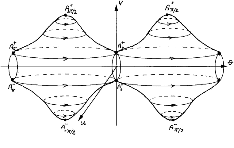
Figure 1: The flow on the collision manifold, which is formed by periodic orbits, eight equilibria, and eight heteroclinic orbits.

3 Heteroclinic Orbits and Bounded Solutions

The flow near the collision manifold was studied in [10], in which most of the results are essentially local. In this section we will prove two global results that extend the understanding of the problem under discussion. The first one concerns the boundedness of solutions on negative energy levels.

Theorem 1

For any negative value of the energy constant, $h<0$, there exists a positive real number $M$ such that any given solution $(r(\tau),v(\tau),\theta(\tau),u(\tau))$ of system (6) satisfies the relation $r<M$.

Proof: Let us assume that there is no $M$ with the above property. Then at least one unbounded solution exists. Since by the energy relation (7), $u^{2}+v^{2}=2r^{2}h+2r\Delta^{-1/2}+2b\Delta^{-1}$, and since $h<0$, there is some $\overline{r}=r(\overline{\tau})$ such that $u^{2}+v^{2}$ is negative—a contradiction. This completes the proof.

The next result deals with the existence of heteroclinic orbits connecting the equilibria but lying outside the collision manifold. But before stating and proving it, let us recall some facts that summarize the behavior of the flow near the collision manifold. Denote by $P_{\eta}$ the periodic orbit on $C$ having $v=\eta$. The following property was proved in [10].

Proposition 1

On the collision manifold $C$ the equilibria $A_{0}^{\pm}$ and $A_{\pi}^{\pm}$ are saddles whereas the equilibria $A_{\pm\pi/2}^{\pm}$ are centers. Outside the collision manifold the equilibria $A_{0}^{\pm}$, $A_{\pm\pi/2}^{+}$, and $A_{\pi}^{+}$ have a $1$-dimensional unstable analytic manifold, whereas the equilibria $A_{0}^{-}$, $A_{\pm\pi/2}$, and $A_{\pi}^{-}$ have a $1$-dimensional stable analytic manifold. Each periodic orbit $P_{\eta}$ on $C$ with $v=\eta>0$($v=\eta<0$) has a $2$-dimensional local unstable analytic manifold, while the periodic orbit $v=0$ has both a $2$-dimensional local unstable and a $2$-dimensional local stable manifold (see Fig. 2)

The above properties are local, the following one, however, is global. We will now show that the equilibria with positive $v$ coordinate have a 1-dimensional global unstable manifold while the equilibria with a negative $v$ have a 1-dimensional stable manifold. Moreover, the equilibria are connected by heteroclinic orbits starting from an equilibrium with positive $v$ and ending in the symmetric one with respect to the $(\theta,u)$ plane.

Theorem 2

There are four heteroclinic orbits outside the collision manifold $C$: $\gamma_{-\pi/2}$ ,$\gamma_{0}$ ,$\gamma_{\pi/2}$ ,$\gamma_{\pi}$ connecting respectively $A_{-\pi/2}^{+}$ with $A_{-\pi/2}^{-}$, $A_{0}^{+}$ with $A_{0}^{-}$, $A_{\pi/2}^{+}$ with $A_{\pi/2}^{-}$, and $A_{\pi}^{+}$ with $A_{\pi}^{-}$ (see Fig. 2)

Proof: First we show that $u=0$ and $\theta=0,\pi,\pm\pi/2$ describe four invariant sets. Consider $\theta(0)=\theta_{0}=0$ and $u(0)=u_{0}=0$, as initial conditions. Then $\theta\equiv 0$, $u\equiv 0$ satisfies system (6), hence (by the uniqueness property for solutions) $u=0$, $\theta=0$ define an invariant set. The same reasoning can be applied if $\theta=\pm\pi/2$ or $\pi$.

Now let’s study the energy relation (7) when $u=0$ and $\theta=0,\pi$. After simple computations we get

$$v^{2}+\left(\sqrt{2|h|}r-{1\over\sqrt{2\mu|h|}}\right)^{2}={2b\over\mu}+{1\over 2\mu|h|}.$$ (10)

The above equation describes an ellipse whose intersections with $r=0$ give $v=\pm\sqrt{2b/\mu}$, which are exactly the equilibrium points $A_{0}^{\pm}$ and $A_{\pi}^{\pm}$. Moreover the maximum value of $|v|$ is

$$v_{max}=\sqrt{{1\over\mu}\Big{(}2b+{1\over 2|h|}\Big{)}}$$ (11)

and the maximum value of $r$, attained when $v=0$, is

$$r_{max}={1\over(2\sqrt{\mu}|h|)}+{\sqrt{{1\over\mu}(1-4hb)}\over 2|h|}.$$ (12)

Consequently for $u=0$, $\theta=0$ ($\theta=\pi$) there exist heteroclinic orbits $\gamma_{0}$, ($\gamma_{\pi}$) ejecting from $A_{0}^{+}$ ($A_{0}^{-}$) and tending to $A_{0}^{-}$ ($A_{\pi}^{-}$) (see Fig. 2).

Similarly when $u=0$ and $\theta=\pm\pi/2$ the energy relation can be reduced to the form

$$v^{2}+\left(\sqrt{2|h|}r-{1\over\sqrt{2|h|}}\right)^{2}=2b+{1\over 2|h|},$$ (13)

which describes an ellipse. The intersections with $r=0$ are $v=\pm\sqrt{2b}$ and represent the equilibria $A_{\pm\pi/2}^{\pm}$. In this case

$$v_{max}=\sqrt{2b+1/2|h|}$$ (14)

and

$$r_{max}={1\over 2|h|}+{\sqrt{1+4b|h|}\over 2|h|}.$$ (15)

Thus we found heteroclinic orbits $\gamma_{\pm\pi/2}$ ejecting from $A_{\pm\pi/2}^{+}$ and tending to $A_{\pm\pi/2}^{-}$ (see Fig. 2). This completes the proof.

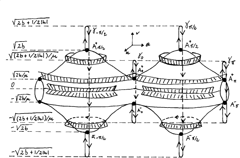
Figure 2: The flow can reach the collision manifold at the equilibria or at any of the periodic orbits. There are four heteroclinic orbits $\gamma_{-\pi/2}$ ,$\gamma_{0}$ ,$\gamma_{\pi/2}$ ,$\gamma_{\pi}$ connecting respectively $A_{-\pi/2}^{+}$ with $A_{-\pi/2}^{-}$, $A_{0}^{+}$ with $A_{0}^{-}$, $A_{\pi/2}^{+}$ with $A_{\pi/2}^{-}$, and $A_{\pi}^{+}$ with $A_{\pi}^{-}$.

4 A Perturbative Approach

We will now write the anisotropic Manev problem as a perturbation of the classical Manev case. Consider weak anisotropies, i.e., choose the parameter $\mu$ close to $1$. Introducing the notation $\mu-1=\epsilon>0$ with $\epsilon\ll 1$, we can expand the equation of motion in powers of $\epsilon$ to obtain

$$\left\{\begin{array}[]{l}r^{\prime}=rv\\ v^{\prime}=2r^{2}h+r-\epsilon(r/2\cos^{2}\theta)\\ \theta^{\prime}=u\\ u^{\prime}=\epsilon(r/2+2b)\sin 2\theta.\end{array}\right.$$ (16)

The energy relation becomes

$$u^{2}+v^{2}-2r-2b+\epsilon(r+2b)\cos^{2}\theta=2r^{2}h.$$ (17)

For $\epsilon=0$, system (16) and equation (17) yield the Manev problem. The collision manifold is the set of solutions given by

$$r=0,\qquad u^{2}+v^{2}=2b.$$ (18)

Notice that, from the geometric point of view, the collision manifold is a cylinder in the three-dimensional space of coordinates $(u,\theta,v)$ and, since $\theta\in[0,2\pi]$, it follows that this cylinder can be identified with a torus. The flow on the collision manifold is formed almost exclusively by non-hyperbolic periodic orbits, except for the upper and lower circles of the torus given by $r=0,\quad u=0,\quad v=\pm\sqrt{2b}$, which consist of equilibrium points. There is only a single orbit ejecting from each fixed point of the upper circle $v=\sqrt{2b}$ and a single orbit tending to the lower circle $v=-\sqrt{2b}$ (see [13]). Moreover it can be easily proved (see [13]) that for every periodic orbit $p_{v}$ on the collision manifold with $0<v<\sqrt{2b}$ there exist a manifold of orbits, lying on a cylinder, which eject from $p_{v}$. Similarly it can be shown that for every orbit $p_{v}$, with $-\sqrt{2b}<v<0$, there exists a manifold of orbits, lying on a cylinder, which tend to $p_{v}$.

If $v=0$ both types of manifolds exist, so $p_{0}$ has a homoclinic manifold. Indeed, the equations that describe the manifold can be found explicitly: they have $u=\pm\sqrt{2b}$. With the energy relation we get

$$v=\pm\sqrt{2r^{2}h+2r},$$ (19)

and using the equation of motion we obtain

$$r^{\prime}=\pm r\sqrt{2r^{2}h+2r}.$$ (20)

By integrating equation (20) it is easy to find that

$$R(\tau-\tau_{0})={2\over 2|h|+(\tau-\tau_{0})^{2}},\quad R^{\prime}=-{4(\tau-\tau_{0})\over(2|h|+(\tau-\tau_{0})^{2})^{2}}$$ (21)

and

$$V(\tau-\tau_{0})={R^{\prime}\over R}=-{2(\tau-\tau_{0})\over 2|h|+(\tau-\tau_{0})^{2}}.$$ (22)

Furthermore

$$U(\tau-\tau_{0})=\pm\sqrt{2b}=\omega\quad\mbox{and}\quad\vartheta(\tau-\tau_{0},\theta_{0})=\Theta(\tau-\tau_{0})-\theta_{0},$$ (23)

where $\Theta(\tau-\tau_{0})=\omega(\tau-\tau_{0})$. As $\tau_{0}$ and $\theta_{0}$ vary, equations (21-23) describe the entire $2$-dimensional homoclinic manifold. An orbit lying on the homoclinic manifold is represented in Fig. 3. Such an orbit is obtained by choosing $\theta_{0}=0$; it ejects from the equator of the collision manifold, spiraling around it and moving upwards, then changes directions, goes downwards and upwards again, spiraling towards the periodic orbit $p_{0}$.

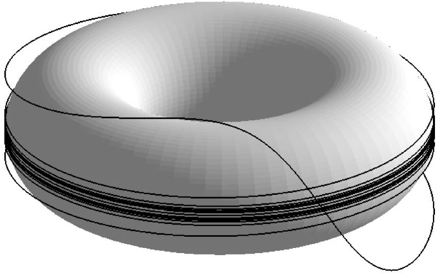
Figure 3: An homoclinic orbit to $p_{0}$ lying on the homoclinic manifold. This orbit spirals out of the equator of the collision manifold and then spirals back to it.

The homoclinic manifold plays an important role in following section and is necessary for developing the generalization of the Melnikov technique.

5 A Generalized Melnikov Method

Let $\chi=(R(\tau),V(\tau),\Theta(\tau),U(\tau))$ be the homoclinic orbit selected when we choose $\tau_{0}=0$ and $\theta_{0}=0$. Consider solutions of the form

$$\left\{\begin{array}[]{l}r(\tau,\tau_{0})=R(\tau-\tau_{0})+\tilde{r}(\tau,\tau_{0})\\ v(\tau,\tau_{0})=V(\tau-\tau_{0})+\tilde{v}(\tau,\tau_{0})\\ \theta(\tau,\tau_{0},\theta_{0})=\Theta(\tau-\tau_{0})-\theta_{0}+\tilde{\theta}(\tau,\tau_{0})\\ u(\tau,\tau_{0})=U(\tau-\tau_{0})+\tilde{u}(\tau,\tau_{0}).\end{array}\right.$$ (24)

Let ${\bf\tilde{z}}=(\tilde{r},\tilde{v},\tilde{\theta},\tilde{u})$, then the variational equation is

$${\bf\tilde{z}}^{\prime}=A(\tau){\bf\tilde{z}}+{\bf\tilde{b}}({\bf\tilde{z}},\chi,\tau,\tau_{0},\theta_{0},\epsilon),$$ (25)

where

$$A(\tau)=\left(\begin{array}[]{cccc}V&R&0&0\\ 1+4Rh&0&0&0\\ 0&0&0&1\\ 0&0&0&0\end{array}\right)$$ (26)

and

$${\bf\tilde{b}}({\bf\tilde{z}},\chi,\tau,\tau_{0},\theta_{0},\epsilon)=\left(\begin{array}[]{c}b_{1}\\ b_{2}\\ b_{3}\\ b_{4}\end{array}\right)=\left(\begin{array}[]{c}\tilde{r}(\tau-\tau_{0})\tilde{v}(\tau-\tau_{0})\\ -\epsilon\left({(R+\tilde{r})\over 2}\cos^{2}(\Theta-\theta_{0}+\tilde{\theta})\right)\\ 0\\ \epsilon\left({(R+\tilde{r})\over 2}+2b\right)\sin 2(\Theta-\theta_{0}+\tilde{\theta})\end{array}\right).$$ (27)

The general solution of the variational equation (25) is

$${\bf\tilde{z}}=\Phi(t)\int_{t_{0}}^{t}\Phi^{-1}(s){\bf\tilde{b}}~{}ds,$$ (28)

(see [18]), where $\Phi$ is the fundamental matrix. If we let $c=\Phi^{-1}{\bf\tilde{b}}$, the previous equation becomes

$$\tilde{z}_{i}(t)=\Phi_{ij}\int_{t_{0}}^{t}c_{j}(s)~{}ds,$$ (29)

where $c_{j}=det~{}D_{j}(t)/(det\Phi)(t)$ and $D_{j}$ is the matrix obtained replacing the $j$-th column of $\Phi$ with ${\bf\tilde{b}}$. Furthermore the following formula for the trace holds:

$$\mbox{det}\Phi(\tau)=Ce^{\int_{\tau_{0}}^{\tau}TrA(s)~{}ds}.$$ (30)

One solution of the homogeneous part of the variational equation is given by

$$\chi^{\prime}(\tau-\tau_{0},\theta_{0})=(R^{\prime}(\tau-\tau_{0}),V^{\prime}(\tau-\tau_{0}),\Theta^{\prime}(\tau-\tau_{0}),U^{\prime}(\tau-\tau_{0})),$$ (31)

where

$$\begin{array}[]{l}R^{\prime}=-{4(\tau-\tau_{0})\over(2|h|+(\tau-\tau_{0})^{2})^{2}}\vskip 3.0pt plus 1.0pt minus 1.0pt\\ V^{\prime}=-{2\over 2|h|+(\tau-\tau_{0})^{2}}+{4(\tau-\tau_{0})^{2}\over(2|h|+(\tau-\tau_{0})^{2})^{2}}\vskip 3.0pt plus 1.0pt minus 1.0pt\\ \Theta^{\prime}=\pm\sqrt{2b}.\vskip 3.0pt plus 1.0pt minus 1.0pt\\ U^{\prime}=0.\end{array}$$ (32)

It is easy to check that other two independent solutions are $(0,0,1,0)$ and $(0,0,0,1)$. Knowing three independent solutions of a linear system, it is possible to find a fourth independent solution $\psi$. This is achieved through the following lemma, which will be used to estimate how fast $\psi$ diverges.

Lemma 1

Let ${\bf\tilde{z}}^{\prime}=A{\bf\tilde{z}}$ be the homogeneous part of (25). Given the three independent solutions above, a fourth is defined by

$$\left\{\begin{array}[]{l}\tilde{z}_{1}^{\prime}=(1+4Rh)/V^{\prime}\tilde{z}_{4}\vskip 3.0pt plus 1.0pt minus 1.0pt\\ \tilde{z}_{2}^{\prime}=\mp{\sqrt{2b}\over V^{\prime}}(1+4Rh)\tilde{z}_{4}\vskip 3.0pt plus 1.0pt minus 1.0pt\\ \tilde{z}_{3}^{\prime}=0\vskip 3.0pt plus 1.0pt minus 1.0pt\\ \tilde{z}_{4}^{\prime}=(V-{R^{\prime}(1+4Rh)\over V^{\prime}})\tilde{z}_{4}\\ \end{array}\right.\qquad\left\{\begin{array}[]{l}\psi_{1}=R^{\prime}\tilde{z}_{1}+\tilde{z}_{4}\vskip 3.0pt plus 1.0pt minus 1.0pt\\ \psi_{2}=V^{\prime}\tilde{z}_{1}\vskip 3.0pt plus 1.0pt minus 1.0pt\\ \psi_{3}=\pm\sqrt{2b}\tilde{z}_{1}+\tilde{z}_{2}\\ \psi_{4}=\tilde{z}_{3}.\end{array}\right.$$ (33)

Proof: To find the fourth independent solution, we can use the “reduction to a smaller system,” (see [18]), whose direct application completes the proof.

In particular it is useful to remark that we can always choose $\psi_{4}=0$, since $(\psi_{1},\psi_{2},\psi_{3},0)$ is a solution that is independent from the other ones. To obtain necessary and sufficient conditions such that the negatively and positively asymptotic sets intersect transversely, we first obtain conditions for the existence of solutions bounded on $\mathbb{R}$ for the non-homogeneous linear variational equation around $\chi$.

For this, let ${\mathcal{B}}({\mathbb{R}})=\{{\bf\tilde{b}}:{\mathbb{R}}\rightarrow\mathbb{R\times R}\times S^{1}\times\mathbb{R}~{}\mbox{bounded, continuous}\}$ with $\|{\bf\tilde{b}}\|=\mbox{sup}_{\tau\in{\mathbb{R}}}\|{\bf\tilde{b}}(\tau)\|$ for ${\bf\tilde{b}}\in\cal{B}({\mathbb{R}})$. Then we have the following version of the Fredholm alternative for solutions bounded on $\mathbb{R}$ (see [5, 6, 8] for a similar approach).

Lemma 2

Let ${\bf\tilde{z}}\in\mathbb{R\times R\times}S^{1}\times\mathbb{R}$ and assume that ${\bf\tilde{z}}\equiv 0$ in the expression of the function ${\bf\tilde{b}}$. Then the variational equation

$${\bf\tilde{z}}^{\prime}=A(\tau){\bf\tilde{z}}+{\bf\tilde{b}}({\bf\tilde{z}},\chi,\tau,\tau_{0},\theta_{0},\epsilon)\quad$$ (34)

has a bounded solution if and only if

$$\int_{-\infty}^{+\infty}e^{-\int_{\tau_{0}}^{\tau}TrA(s)ds}~{}R^{\prime}(\tau-\tau_{0})~{}b_{2}(\chi,\tau,\tau_{0},\theta_{0},\epsilon)~{}d\tau=0.$$ (35)

The solution is unique and continuous and has the form ${\bf\tilde{z}}={\bf L}({\bf\tilde{b}})+{\bf w}$, where ${\bf L}$ is a bounded linear operator, ${\bf w}=(0,0,\tilde{\theta}(\tau_{0}),\tilde{u}(\infty))$, when $\tilde{r}(\tau_{0})R^{\prime}(\tau_{0})+\tilde{v}(\tau_{0})V^{\prime}(\tau_{0}))=0$, and $b_{4}$ satisfies the relation below,

$$\int_{-\infty}^{+\infty}b_{4}(\chi,\tau,\tau_{0},\theta_{0},\epsilon)~{}d\tau=0.$$ (36)

Proof: Using Lemma 1 it is easy to determine the behavior of $\psi$ as $\tau\rightarrow\pm\infty$, precisely,

$$\tau\rightarrow\pm\infty\left\{\begin{array}[]{l}\tilde{z}_{1}\sim\tau^{4}\\ \tilde{z}_{2}\sim\tau^{4}\\ \tilde{z}_{3}\sim\mbox{const.}\\ \tilde{z}_{4}\sim\tau,\\ \end{array}\right.\quad\quad\tau\rightarrow\pm\infty\left\{\begin{array}[]{l}\psi_{1}\sim\tau\\ \psi_{2}\sim\tau^{2}\\ \psi_{3}\sim\tau^{4}\\ \psi_{4}\sim\mbox{const.}\\ \end{array}\right.$$ (37)

Using (29) and (30), the general solution of the complete (non-homogeneous) equation (25) can be written in integral form as

$$\begin{split}\tilde{r}&=R^{\prime}\left(A-\int_{\tau_{0}}^{\tau}e^{-\int_{s_{0}}^{s}TrA(\eta)d\eta}(\psi_{1}b_{2}-\psi_{2}b_{1})~{}ds\right)\\ &+\psi_{1}\left(B+\int_{\tau_{0}}^{\tau}e^{-\int_{s_{0}}^{s}TrA(\eta)d\eta}(R^{\prime}b_{2}-V^{\prime}b_{1})~{}ds\right)\\ \tilde{v}&=V^{\prime}\left(A-\int_{\tau_{0}}^{\tau}e^{-\int_{s_{0}}^{s}TrA(\eta)d\eta}(\psi_{1}b_{2}-\psi_{2}b_{1})~{}ds\right)\\ &+\psi_{2}\left(B+\int_{\tau_{0}}^{\tau}e^{-\int_{s_{0}}^{s}TrA(\eta)d\eta}(R^{\prime}b_{2}-V^{\prime}b_{1})~{}ds\right)\\ \tilde{\theta}&=\pm\sqrt{2b}\left(A-\int_{\tau_{0}}^{\tau}e^{-\int_{s_{0}}^{s}TrA(\eta)d\eta}(\psi_{1}b_{2}-\psi_{2}b_{1})~{}ds\right)\\ &+\psi_{3}\left(B+\int_{\tau_{0}}^{\tau}e^{-\int_{s_{0}}^{s}TrA(\eta)d\eta}(R^{\prime}b_{2}-V^{\prime}b_{1})~{}ds\right)\\ &+C-\int_{\tau_{0}}^{\tau}e^{-\int_{s_{0}}^{s}TrA(\eta)d\eta}\left[(-V^{\prime}\psi_{3}\pm\sqrt{2b}\psi_{2})b_{1}+(R^{\prime}\psi_{3}\pm\sqrt{2b}\psi_{1})b_{2}\right]\\ \tilde{u}&=~{}D+\int_{\tau_{0}}^{\tau}b_{4}~{}ds,\end{split}$$ (38)

where, for notational convenience, we failed to mention the dependence on ${\bf\tilde{z}}$, $\chi$, $\tau_{0}$, etc.

Consider now the linearization of the problem (38) around the solution ${\bf\tilde{z}(\tau)}\equiv 0$; in particular this amounts to deleting the high-order terms in the expression of ${\bf\tilde{b}}$ (i.e. $b_{1}=0$, etc.). Taking also into account the different behavior of the different solutions given in Lemma 1, it is easy to see that to have bounded solutions we need to require that

$$\psi_{i}\left(A-\int_{\tau_{0}}^{\tau}e^{-\int_{s_{0}}^{s}TrA(\eta)d\eta}\psi_{1}b_{2}(\chi,s,\tau_{0},\theta_{0},\epsilon)~{}ds\right)\qquad\mbox{for}~{}i=1,\dots,4,$$ (39)

remains bounded as $\tau\rightarrow\pm\infty$. More precisely ${\bf\tilde{z}}$ is bounded on $[\tau_{0},\infty)$ if and only if

$$A=\int_{\tau_{0}}^{\infty}e^{-\int_{s_{0}}^{s}TrA(\eta)d\eta}\psi_{1}b_{2}~{}ds$$ (40)

and bounded on $(-\infty,\tau_{0}]$ if and only if

$$A=-\int_{-\infty}^{\tau_{0}}e^{-\int_{s_{0}}^{s}TrA(\eta)d\eta}\psi_{1}b_{2}~{}ds.$$ (41)

We also require

$$\tilde{u}(\pm\infty)=\lim_{\tau\to\ \pm\infty}\tilde{u}(\tau)=D+\lim_{\tau\to\pm\infty}\int_{\tau_{0}}^{\tau}b_{4}(\chi,s,\tau_{0},\theta_{0},\epsilon)~{}ds,$$ (42)

where, obviously, $\tilde{u}(\infty)=\tilde{u}(-\infty)$. The latter condition is not needed for the boundedness of the solution, but its role will be clear later when analyzing some properties of the negatively and positively asymptotic sets. It is easy to see that the above conditions are simultaneously satisfied both at $\tau=-\infty$ and at $\tau=+\infty$ if for some $\tau_{0}$ the following Melnikov-type conditions:

$$\begin{split}&\int_{-\infty}^{+\infty}e^{-\int_{\tau_{0}}^{\tau}TrA(\eta)~{}d\eta}\psi_{1}b_{2}(\chi,s,\tau_{0}.\theta_{0},\epsilon)~{}ds=0\\ &\int_{-\infty}^{+\infty}b_{4}(\chi,s,\tau_{0},\theta_{0},\epsilon)~{}ds=0\end{split}$$ (43)

are fulfilled. Thus we can rewrite the general solution (38) using (43) and, by neglecting to mention the dependence on $\chi$, $s$, etc., we obtain

$$\begin{split}\tilde{r}&=-R^{\prime}\int_{\infty}^{\tau}e^{-\int_{s_{0}}^{s}TrA(\eta)d\eta}\psi_{1}b_{2}~{}ds+\psi_{1}\left(B+\int_{\tau_{0}}^{\tau}e^{-\int_{s_{0}}^{s}TrA(\eta)d\eta}R^{\prime}b_{2}~{}ds\right)\\ \tilde{v}&=-V^{\prime}\int_{\infty}^{\tau}e^{-\int_{s_{0}}^{s}TrA(\eta)d\eta}\psi_{1}b_{2}~{}ds+\psi_{2}\left(B+\int_{\tau_{0}}^{\tau}e^{-\int_{s_{0}}^{s}TrA(\eta)d\eta}R^{\prime}b_{2}~{}ds\right)\\ \tilde{\theta}&=\mp\sqrt{2b}\int_{\infty}^{\tau}e^{-\int_{s_{0}}^{s}TrA(\eta)d\eta}\psi_{1}b_{2}~{}ds+\psi_{3}\left(B+\int_{\tau_{0}}^{\tau}e^{-\int_{s_{0}}^{s}TrA(\eta)d\eta}R^{\prime}b_{2}~{}ds\right)\\ &+C-\int_{\tau_{0}}^{\tau}e^{-\int_{s_{0}}^{s}TrA(\eta)d\eta}(R^{\prime}\psi_{3}\pm\sqrt{2b}\psi_{1})b_{2}\\ \tilde{u}&=~{}\tilde{u}({\infty})+\int_{\infty}^{\tau}b_{4}~{}ds.\end{split}$$ (44)

To obtain $\tilde{r}(\tau_{0})R^{\prime}(\tau_{0})+\tilde{v}(\tau_{0})V^{\prime}(\tau_{0}))=0$ we must have

$$B={(R^{\prime 2}(\tau_{0})+V^{\prime 2}(\tau_{0}))\over\psi_{1}(\tau_{0})R^{\prime}(\tau_{0})+\psi_{2}(\tau_{0})V^{\prime}(\tau_{0})}\int_{\infty}^{\tau_{0}}\psi_{1}(s)b_{2}(s)~{}ds.$$ (45)

Moreover we also get

$$C=\tilde{\theta}(\tau_{0})\pm\sqrt{2b}\int_{\infty}^{\tau_{0}}e^{-\int_{s_{0}}^{s}TrA(\eta)d\eta}\psi_{1}b_{2}~{}ds\\$$ (46)

and

$$D=\tilde{u}(\infty)+\int_{\infty}^{\tau_{0}}b_{4}~{}ds.$$ (47)

This uniquely defines $B$, $C-\tilde{\theta}(\tau_{0})$, and $D-\tilde{u}(\infty)$ as continuous linear functionals on ${\cal B}(\mathbb{R})$. From (44) we observe that the corresponding solution is of the form ${\bf\tilde{z}}={\bf L}({\bf\tilde{b}})+{\bf w}$, where ${\bf L}$ is a bounded linear operator. It follows that this operator is continuous and hence the solution ${\bf\tilde{z}}={\bf L}({\bf\tilde{b}})+{\bf w}$ is continuous on ${\cal B}(\mathbb{R})$. This completes the proof.

To obtain necessary and sufficient conditions that the negatively and positively asymptotic sets intersect, let us first consider all the solutions of (25) which are bounded as $\tau\rightarrow-\infty$ and such that their angles remain close to the ones on the periodic orbit. The solution ${\bf\tilde{z}}$ is given by (38) satisfying (41) and (42) with negative sign. In particular the solutions of the variational equation that are bounded as $\tau\rightarrow-\infty$ (i.e. which remain in a sufficiently small neighborhood of the periodic orbit as $\tau\rightarrow-\infty$) and with perturbed angles that do not drift but remain near the angles on the periodic orbit, must be on the negatively asymptotic set. In the same way, we obtain the positively invariant set from the solutions that remain bounded as $\tau\rightarrow\infty$ and whose angles stay close to the one of the periodic orbit, which was in fact the reason why we required that condition (42) be satisfied.

Moreover it is important to remark that the solution we found are not only bounded but also such that $\tilde{r}\rightarrow 0$, $\tilde{v}\rightarrow 0$ as $\tau\rightarrow\infty$ and this is important since, on the collision manifold we have many periodic orbit and this condition is needed to show that the orbits are actually asymptotic to the equator.

With the preparations above, we can now prove the following result.

Theorem 3

System (16) has transversal homoclinic solutions if and only if there exist $\tau_{0}^{*}$ and a $\theta_{0}^{*}$ such that

$$\tilde{M}_{1}(\tau_{0}^{*},\theta_{0}^{*})=\tilde{M}_{2}(\tau_{0}^{*},\theta_{0}^{*})=0\quad\mbox{and}\quad{\partial\tilde{M}_{1}\over\partial\tau_{0}}{\partial\tilde{M}_{2}\over\partial\theta_{0}}-{\partial\tilde{M}_{1}\over\partial\theta_{0}}{\partial\tilde{M}_{2}\over\partial\tau_{0}}\left|{}_{\begin{subarray}{c}\tau_{0}=\tau_{0}^{*}\\ \theta_{0}=\theta_{0}^{*}\end{subarray}}\right.\neq 0,$$ (48)

where

$$\begin{split}\tilde{M}_{1}(\tau_{0},\theta_{0})&=\int_{-\infty}^{+\infty}e^{-\int_{\tau_{0}}^{\tau}TrA(s)ds}~{}R^{\prime}~{}b_{2}({\bf\tilde{z}}^{*},\tau,\tau_{0},\theta_{0},\epsilon)~{}d\tau,\\ \tilde{M}_{2}(\tau_{0},\theta_{0})&=\int_{-\infty}^{+\infty}b_{4}({\bf\tilde{z}}^{*},\tau,\tau_{0},\theta_{0},\epsilon)~{}d\tau,\end{split}$$ (49)

and ${\bf\tilde{z}}^{*}$ is a solution of ${\bf\tilde{z}}={\bf L}({\bf\tilde{b}}({\bf\tilde{z}},\tau,\tau_{0},\theta_{0},\epsilon))+{\bf w}$. Moreover if the perturbation is periodic we get infinitely many intersections.

Proof: The stable and unstable manifolds intersect if and only if the solution (38) satisfies the Melnikov-like conditions (35) and (42) of Lemma 2. This was already proved in the case when ${\bf\tilde{b}}$ did not implicitly depend depend on ${\bf\tilde{z}}$. But because of this implicit dependence we need to apply the implicit function theorem, which states that given ${\bf\tilde{z}}={\bf L}({\bf\tilde{b}}({\bf\tilde{z}},\tau,\tau_{0},\theta_{0},\epsilon))+{\bf w}$ with ${\bf\tilde{z}-w}={\bf L}(0,\tau,\tau_{0},\theta_{0},0)=0$, there exist a $\delta$ and a unique solution ${\bf\tilde{z}^{*}(\epsilon,\tau_{0},\theta_{0})}$ (that has continuous derivatives up to order 2 in $\tau_{0},\theta_{0},\epsilon$) such that $\epsilon<0$, $|{\bf\tilde{z}}|<\delta$ if the linearized operator ${\bf\tilde{z}}={\bf L}({\bf\tilde{b}}(0,\tau,\tau_{0},\theta_{0},\epsilon))+{\bf w}$ is invertible. But Lemma 2 proved that such an operator is invertible. Moreover the homoclinic solutions are transversal if and only if the integrals (49) have simple zeroes, as functions of $\tau_{0}$ and $\theta_{0}$ (see [5, 6]). This concludes the proof.

Unfortunately the Melnikov integrals of Theorem 3 are difficult to compute explicitly. To overcome this difficulty we need to rewrite these integrals to the first order approximation in $\epsilon$. Hence if we let ${\bf\tilde{z}}^{*}=\epsilon\chi$ and ${\bf\tilde{b}}=\epsilon{\bf d}$ with ${\bf d}=(d_{1},d_{2},d_{3},d_{4})$, the next result follows immediately.

Corollary 1

System (16) has transversal homoclinic solutions if and only if there exist $\tau_{0}^{*}$ and a $\theta_{0}^{*}$ such that

$$M_{1}(\tau_{0}^{*},\theta_{0}^{*})=M_{2}(\tau_{0}^{*},\theta_{0}^{*})=0\quad\mbox{and}\quad{\partial M_{1}\over\partial\tau_{0}}{\partial M_{2}\over\partial\theta_{0}}-{\partial M_{1}\over\partial\theta_{0}}{\partial M_{2}\over\partial\tau_{0}}\left|{}_{\begin{subarray}{c}\tau_{0}=\tau_{0}^{*}\\ \theta_{0}=\theta_{0}^{*}\end{subarray}}\right.\neq 0,$$ (50)

where

$$\begin{split}M_{1}(\tau_{0},\theta_{0})&=\int_{-\infty}^{+\infty}e^{-\int_{\tau_{0}}^{\tau}TrA(s)ds}~{}R^{\prime}(\tau-\tau_{0})~{}b_{2}(\chi(\tau-\tau_{0}),\Theta(\tau-\tau_{0})-\theta_{0})~{}d\tau,\\ M_{2}(\tau_{0},\theta_{0})&=\int_{-\infty}^{+\infty}b_{4}(\chi(\tau-\tau_{0}),\Theta(\tau-\tau_{0})-\theta_{0})~{}d\tau.\end{split}$$ (51)

Moreover if the perturbation is periodic we get infinitely many intersections.

Corollary 1 generalizes the Melnikov integrals obtained in [19, 28] to nonhyperbolic whiskered tori (periodic orbits) in non-Hamiltonian systems. We remark that the second integral in (51) converges only conditionally. This is not a new feature of this non-Hamiltonian system since the same nuisance was present in [19, 28]. However some authors, more recently, found a way to write the Melnikov conditions for hyperbolic whiskered tori in Hamiltonian systems using only convergent integrals see [12, 27]. It would be interesting to generalize those results to nonhyperbolic tori in non-Hamiltonian systems and to apply the newly developed technique to the problem under discussion in this paper. But this is not a project we aim to develop here.

6 The Melnikov Integrals

Now we would like to apply Corollary 1 to our problem. The Melnikov conditions take the form

$$\begin{split}M_{1}(\tau_{0},{\theta}_{0})=\int_{-\infty}^{+\infty}\Big{[}e^{-{1\over 2}\int_{\tau_{0}}^{\tau}V(s)ds}R(\tau-\tau_{0})R^{\prime}(\tau-\tau_{0})\\ \times\cos^{2}(\omega(\tau-\tau_{0})-{\theta}_{0})\Big{]}~{}d\tau=0\end{split}$$ (52)

and

$$M_{2}(\tau_{0},{\theta}_{0})={1\over 2}\int_{-\infty}^{+\infty}(R(\tau-\tau_{0})+2b)\sin(2(\omega(\tau-\tau_{0})-{\theta}_{0}))~{}d\tau=0.$$ (53)

Let $\tilde{\theta}_{0}=-{\theta}_{0}-\omega\tau_{0}$. With this assumption we can rewrite the first Melnikov condition as

$$M_{1}=\cos^{2}\tilde{\theta}_{0}I_{1}^{a}+\sin^{2}\tilde{\theta}_{0}I_{1}^{b}-\sin 2\theta_{0}I_{1}^{c},$$ (54)

where

$$\left\{\begin{array}[]{l}I_{1}^{a}=\int_{-\infty}^{+\infty}e^{-{1\over 2}\int_{\tau_{0}}^{\tau}V(s)ds}RR^{\prime}\cos^{2}\omega\tau~{}d\tau\vskip 6.0pt plus 2.0pt minus 2.0pt\\ I_{1}^{b}=\int_{-\infty}^{+\infty}e^{-{1\over 2}\int_{\tau_{0}}^{\tau}V(s)ds}RR^{\prime}\sin^{2}\omega\tau~{}d\tau\vskip 6.0pt plus 2.0pt minus 2.0pt\\ I_{1}^{c}=\int_{-\infty}^{+\infty}e^{-{1\over 2}\int_{\tau_{0}}^{\tau}V(s)ds}RR^{\prime}\sin\omega\tau\cos\omega\tau~{}d\tau.\end{array}\right.$$ (55)

The second Melnikov condition can be expressed as

$$M_{2}=\cos 2\tilde{\theta}_{0}I_{2}^{a}+\sin 2\tilde{\theta}_{0}I_{b}^{2},$$ (56)

where

$$\left\{\begin{array}[]{l}I_{2}^{a}={1\over 2}\int_{-\infty}^{+\infty}(R+2b)\sin 2\omega\tau~{}d\tau\vskip 6.0pt plus 2.0pt minus 2.0pt\\ I_{2}^{b}={1\over 2}\int_{-\infty}^{+\infty}(R+2b)\cos 2\omega\tau~{}d\tau.\\ \end{array}\right.$$ (57)

All the integrals above can be computed using the method of residues. Straightforward computations give

$$I_{1}^{a}=-I_{1}^{b}={-1\over|h|}\int_{-\infty}^{+\infty}{(\tau-\tau_{0})\cos 2\omega\tau\over(2|h|+(\tau-\tau_{0})^{2})^{2}}~{}d\tau={\pi\sin(2\omega\tau_{0})e^{-2\omega\sqrt{2|h|}}\over|h|\sqrt{2|h|}}$$ (58)

and

$$I_{1}^{c}={-1\over|h|}\int_{-\infty}^{+\infty}{(\tau-\tau_{0})\sin\omega\tau\cos\omega\tau\over(2|h|+(\tau-\tau_{0})^{2})^{2}}~{}d\tau=-{\pi\cos(2\omega\tau_{0})e^{-2\omega\sqrt{2|h|}}\over|h|\sqrt{2|h|}}.$$ (59)

Particular care is needed when integrating $I_{2}^{a}$ and $I_{2}^{b}$ since they converge only conditionally. To obtain computational convergence, we choose the limits in $I_{2}^{a}$ such that

$$\begin{split}I_{2}^{a}&=\lim_{N\to\infty}\int_{-N\pi/2\omega}^{N\pi/2\omega}\left(b+{1\over 2|h|+(\tau-\tau_{0})^{2}}\right)\sin 2\omega\tau~{}d\tau\\ &={\pi\sin(2\omega\tau_{0})e^{-2\omega\sqrt{2|h|}}\over\sqrt{2|h|}}.\end{split}$$ (60)

The integral was also computed using the method of residues. Similarly, for $I_{2}^{b}$, we have

$$\begin{split}I_{2}^{b}&=\lim_{N\to\infty}\int_{-N\pi/2\omega}^{N\pi/2\omega}\left(b+{1\over 2|h|+(\tau-\tau_{0})^{2}}\right)\cos 2\omega\tau~{}d\tau\\ &={\pi\cos(2\omega\tau_{0})e^{-2\omega\sqrt{2|h|}}\over\sqrt{2|h|}}\end{split}$$ (61)

and thus

$$M_{1}=M_{2}=\sin(2(\omega\tau_{0}+\tilde{\theta}_{0})){\pi e^{-2\omega\sqrt{2|h|}}\over\sqrt{2|h|}}.$$ (62)

We therefore have only one independent condition; this is clearly a consequence of the energy relation.

We can find simple zeroes when $\sin(2(\omega\tau_{0}+\tilde{\theta}_{0}))=0$, i.e., for $-(\omega\tau_{0}+\tilde{\theta}_{0})=\theta_{0}=\pm k\pi/2$ for $k=0,1,2,\dots$.

Hence, by Corollary 1, we have proved the existence of an infinite sequence of intersections on the Poincaré section of the negatively and positively asymptotic sets of the periodic orbit and the existence of homoclinic orbits leaving the equator of the collision manifold and going back to it. This situation is clearly reminiscent of the chaotic dynamics described by the Poincaré-Birkhoff-Smale theorem in terms of symbolic dynamics and the Smale horseshoe. Unfortunately this theorem cannot be directly applied, nor can the theorems proved in [1], since the Poincaré-Birkhoff-Smale theorem considers hyperbolic fixed points while the arguments in [1] apply to area-preserving diffeomorphisms. However the arguments contained in those theorems strongly suggest the occurrence of a chaotic dynamics.

Moreover it is easy to verify, and interesting to remark, that the orbits we found above are not $\overline{S}_{0}$-symmetric, where the $\overline{S}_{0}$ symmetry is defined by $\overline{S}_{0}(r,v,\theta,u,\tau)=(r,-v,-u,-\tau)$ (see [10]) and an orbit $\gamma(\tau)$ is said to be $\overline{S}_{0}$-symmetric if $\overline{S}_{0}(\gamma(\tau))=\gamma(\tau)$. Indeed an orbit is $\overline{S}_{0}$-symmetric if and only if it has a point on the zero velocity curve, i.e., if there is a $\overline{\tau}$ such that $v(\overline{\tau})=u(\overline{\tau})=0$ (see [24]). But this cannot happen in our problem because the unperturbed solution verifies $u\equiv\pm\sqrt{2b}$. Thus for $\epsilon$ small enough the perturbed orbit can never have $u=0$.

We can now summarize the above discussion as follows:

Theorem 4

Let us consider the anisotropic Manev problem given by the equation of motion (6) with the energy relation (7). Then there is an infinite sequence of intersections in the Poincaré section of the negatively and positively asymptotic sets of the periodic orbits at the equator of the collision manifold (possibly giving rise to a chaotic dynamics). Furthermore there exist the homoclinic non $\overline{S}_{0}$-symmetric orbits to the periodic orbit described above.

7 Periodic Solutions

We now return to the original Cartesian coordinates, which are more convenient for the purpose of finding certain periodic solutions. Let us first notice that the equations (2) admit the following symmetries:

$$\begin{array}[]{l}S_{0}(x,y,p_{x},p_{y},t)=(x,y,-p_{x},-p_{y},-t),\\ S_{1}(x,y,p_{x},p_{y},t)=(x,-y,-p_{x},p_{y},-t),\\ S_{2}(x,y,p_{x},p_{y},t)=(-x,y,p_{x},-p_{y},-t),\\ S_{3}(x,y,p_{x},p_{y},t)=(-x,-y,-p_{x},-p_{y},t),\\ S_{4}(x,y,p_{x},p_{y},t)=(-x,y,-p_{x},p_{y},t),\\ S_{5}(x,y,p_{x},p_{y},t)=(x,-y,p_{x},-p_{y},t),\\ S_{6}(x,y,p_{x},p_{y},t)=(-x,-y,p_{x},p_{y},-t),\end{array}$$

which are the elements of an Abelian group of order eight, isomorphic to ${\bf Z}_{2}\times{\bf Z}_{2}\times{\bf Z}_{2}$, that is generated by $S_{0},S_{1},S_{2}$ (see [24]). (The symmetry $S_{0}$ is the one denoted by $\overline{S}_{0}$ in the McGehee coordinates of the previous section.) To obtain certain families of periodic solutions, we will use the symmetries $S_{0}$,$S_{1}$ and $S_{2}$ in connection with the variational principle according to which extremum values of the action integral yield periodic solutions of the equations (2). To reach this goal we first need to introduce some notations.

Let $C^{\infty}([0,T],\mathbb{R}^{2})$ be the space of $T$-periodic $C^{\infty}$ cycles $f:[0,T]\rightarrow\mathbb{R}^{2}$. Define the inner products

$$\begin{array}[]{l}\langle f,g\rangle_{L^{2}}=\int_{0}^{T}f(t)\cdot g(t)dt,\vskip 6.0pt plus 2.0pt minus 2.0pt\\ \langle f,g\rangle_{H^{1}}=\langle f,g\rangle_{L^{2}}+\langle\dot{f},\dot{g}\rangle_{L^{2}},\end{array}$$ (63)

and let $\|\cdot\|_{L^{2}}$, $\|\cdot\|_{H^{1}}$ be the corresponding norms. Then the completion of $C^{\infty}([0,T],\mathbb{R}^{2})$ with respect to the norm $\|\cdot\|_{L^{2}}$ is denoted by $L^{2}$ and it is the space of square integrable functions. The completion with respect to $\|\cdot\|_{H^{1}}$ is denoted by $H^{1}$ and is the Sobolev space of all absolutely continuous $T$-periodic paths that have $L^{2}$ derivatives defined almost everywhere (see [16]).

Let $\Sigma_{i}([0,T],\mathbb{R}^{2})$ denote the subset of $H^{1}$ formed by the $S_{i}$-symmetric paths, with $i\in\{0,1,2,3,4,5,6\}$. It is easy to see that each $\Sigma_{i}$ is a subspace of $H^{1}$; in fact they are Sobolev spaces and have many interesting properties. In the following we will restrict our attention to the spaces $\Sigma_{i}$ with $i=0,1,2,6$. Let us now prove the following result.

Lemma 3

Let $H^{1}$ be defined as above, then the subspaces $\Sigma_{i}$ of $S_{i}$-symmetric paths with $i=0,1,2,6$ are closed, weakly closed, and complete with respect to the norm $\|\cdot\|_{H^{1}}$, and are therefore Sobolev spaces. Moreover

$$H^{1}=\Sigma_{1}\oplus\Sigma_{2}=\Sigma_{0}\oplus\Sigma_{6}.$$ (64)

Proof: We first show an interesting fact: we can write $f=(f^{1},f^{2})$ as the sum of an $S_{1}$ and an $S_{2}$-symmetric path. Indeed it is well known that we can write $f_{1}$ and $f_{2}$ as the sum of an even and an odd absolutely continuous function, i.e. as $f_{1}=f_{1}^{e}+f_{1}^{o}$ and $f_{2}=f_{2}^{e}+f_{2}^{o}$. Using this idea we can write the path $f(t)$ as the sum of an $S_{1}$-symmetric function, $f_{S_{1}}=(f_{1}^{e},f_{2}^{o})$, and an $S_{2}$-symmetric one, $f_{S_{2}}=(f_{1}^{o},f_{2}^{e})$. Now fix an element $f\in\Sigma_{1}$. Then $\langle f,g\rangle_{H^{1}}=0$ for every $g\in\Sigma_{2}$. This is because

$$\langle f,g\rangle_{H^{1}}=\int_{0}^{T}(f_{1}g_{1}+f_{2}g_{2})~{}dt~{}+~{}\int_{0}^{L}(f_{1}^{\prime}g_{1}^{\prime}+f_{2}^{\prime}g_{2}^{\prime})~{}dt,$$

where the first integrand is an odd function and the second is an odd function almost everywhere. Thus the above scalar product is zero for every $g\in\Sigma_{2}$.

Let us denote the space orthogonal to $\Sigma_{1}$ by $\Sigma_{1}^{\bot}=\{g\in\Sigma_{1}:\langle f,g\rangle_{H^{1}}=0~{}\mbox{for every}~{}g\in\Sigma_{1}\}$. It is easy to see that $\Sigma_{1}^{\bot}$ is closed and that $S_{2}\subset\Sigma_{1}^{\bot}$. Now we need to show that $S_{2}\supset\Sigma_{1}^{\bot}$. Assume there is $h\in\Sigma_{1}^{\bot}$ such that $h\neq 0$ and $h\in\Sigma_{2}$. Then write $h=h_{S_{1}}+h_{S_{2}}$ and consider $\langle h_{S_{1}},h_{S_{1}}+h_{S_{2}}\rangle_{H^{1}}$, which means that $\langle h_{S_{1}},h_{S_{1}}\rangle_{H^{1}}=\|h_{S_{1}}\|=\delta>0$. But this contradicts the hypothesis that $h\in\Sigma_{1}^{\bot}$. Therefore $\Sigma_{2}=\Sigma_{1}^{\bot}$. So $\Sigma_{2}$ and consequently $\Sigma_{1}$ are closed and such that $H^{1}=\Sigma_{1}\oplus\Sigma_{2}$. Moreover, since $H^{1}$ is a metric space, $\Sigma_{1}$ and $\Sigma_{2}$ are complete. Also $\Sigma_{1}$ and $\Sigma_{2}$ are weakly closed since they are norm-closed subspaces. The statements for $\Sigma_{0}$ and $\Sigma_{6}$ can be proved in a similar way. This completes the proof.

Let us now introduce some new definitions. We will say that a path in $\Sigma_{i}$ is of class $L_{n}$, $n=0,\pm 1,\pm 2,\pm 3,\dots$, if its winding number about the origin of the coordinate system is $n$ (i.e. if it makes $n$ loops around the origin). The sign of $n$ is positive for a counterclockwise rotation and negative otherwise. Consider the sets $\overline{\Sigma}_{i}([0,T],\mathbb{R}^{2}\backslash\{0\})$. Notice that they are open submanifolds of the spaces $\Sigma_{i}([0,T],\mathbb{R}^{2})$ and that the family $(L_{n})_{n\in{\bf Z}}$ provides a partition of those spaces into homotopy classes, also called components. Two periodic orbits of the isotropic Manev problem ($\mu=1$), one of class $L_{8}$ and the other of class $L_{-9}$, are depicted in Fig. 4.

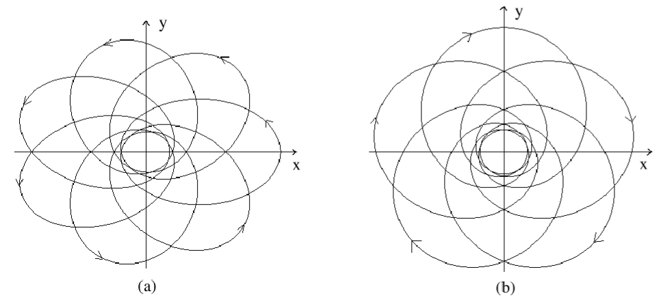
Figure 4: Periodic orbits of the Manev problem: (a) $S_{1}$-symmetric periodic orbit of class $L_{8}$, (b) $S_{2}$-symmetric periodic orbit of class $L_{-9}$. Note that none of these two is $S_{3}$ symmetric.

The Lagrangian $L({\bf q},{\dot{\bf q}})=T({\dot{\bf q}})+U({\bf q})$ of the anisotropic Manev problem given by system (2) has the expression

$$L(x,y,{\dot{x}},{\dot{y}})={1\over 2}({\dot{x}}^{2}+{\dot{y}}^{2})+{1\over\sqrt{x^{2}+\mu y^{2}}}+{b\over x^{2}+\mu y^{2}},$$ (65)

and the action integral along a path $f$ from time $0$ to time $T$, whose Euclidean coordinate representation is ${\bf q}={\bf q}(t)=(x(t),y(t))$, takes the form

$$A_{T}(f)=\int_{0}^{T}L({\bf q}(t),{\bf\dot{q}}(t))dt.$$

According to Hamilton’s principle, the extremals of the functional $A_{T}$ are solutions of the equations (2). Hence we want to obtain periodic solutions of (2) by finding extremals of the functional $A$. For this we will use a direct method of the calculus of variation, namely the lower-semicontinuity method (see [25]). In preparation of a satisfactory theory of existence, the notion of admissible function has to be relaxed since the extremals we obtain belong to a Sobolev space. Therefore the above method provides only “weak” solutions of our problem. To show that the paths are regular enough to be classical solutions, we need the following result, proved in [16].

Lemma 4

The critical points of $A_{T}|_{\overline{\Sigma}_{i}([0,T],\mathbb{R}^{2}\backslash\{0\})}$ are $T$-periodic solutions of equations (2).

In particular it is well known that if $f$ is a minimizer of the action $A_{T}$ in the space $H^{1}([0,t],\mathbb{R}^{2})$ and if $f$ has no collisions, then $f$ is a $T$-periodic solution to (2). Collision have to be excluded because equations (2) break down at collisions and because the action is not differentiable at paths with collisions. In this paper we are interested to restrict ourself to the spaces $\Sigma_{i}$ of $S_{i}$-symmetric paths for $i=0,1,2$. The paths that are $S_{6}$-symmetric have to be excluded in the study of periodic orbits since $S_{6}$-symmetric paths must intersect the origin and therefore encounter collisions.

Now it is not obvious that a collisionless minimizer in $\Sigma_{i}$ is a periodic solution of system (2). However, according to the principle of “symmetric criticality” (see for example [3, 22]) this is actually true. Indeed, it can be proved that if $f$ is a collision free path with $dA_{t}(f)(h)=0$ for every $f\in\Sigma_{i}$, then $dA_{T}(f)(h)=0$ for all $f\in H^{1}([0,T],\mathbb{R}^{2})$ and thus $f$ is a critical point in the bigger loop space $H^{1}$ (see [3]).

The only obstacle left for applying the direct method is the “noncompactness” of the configuration space. Indeed we want to exclude the possibility that the minimizer is obtained when the bodies are at infinite distance from each other or are collision paths. The first problem is solved restricting ourselves to non-simple cycles, i.e., to cycles that are not homotopic to a point and thus are not in the homotopy class $L_{0}$. The second problem is solved by the following result.

Lemma 5

Any family $\Gamma$ of non-simple homotopic cycles in $\overline{\Sigma}_{i}([0,T],\mathbb{R}^{2}\backslash\{0\})$ for $i=0,1,2$ on which $J(f)=\int_{0}^{T}{1\over 2}|{\bf\dot{q}}(t)|^{2}dt$ and $E(f)=\int_{0}^{T}U({\bf q}(t))dt$ are bounded, is bounded away from the origin.

The proof of this result follows from [16] if we remark that the anisotropic Manev potential is “strong” according to Gordon’s definition and that the Lagrangian is positive.

To apply the direct method we still need to recall some properties of lower semicontinuous (l.s.c) functions. Let ${\cal F}:X\rightarrow\mathbb{R}$ be a real valued function on a topological space $X$. Then $\cal{F}$ is l.s.c. if and only if ${\cal F}^{-1}(-\infty,a]$ is closed for every $a\in\mathbb{R}$, in which case $\cal{F}$ is bounded below and attains its infimum on every compact subset of $X$. Moreover when $X$ is Hausdorff then compact sets are necessarily closed and thus we have the following result.

Proposition 2

Suppose ${\cal F}:X\rightarrow\mathbb{R}$ is a real valued function on an Hausdorff space $X$ and

$${\cal F}^{-1}(-\infty,b]~{}\mbox{ is compact for every real b}.$$

Then ${\cal F}$ is l.s.c., bounded below, and attains its infimum value on $X$.

We can now prove the main result of this section.

Theorem 5

For any $T>0$ and any $n=\pm 1,\pm 2,\pm 3,\dots$, there is at least one $S_{i}$-symmetric ($i=0,1,2$) periodic orbit of the anisotropic Manev problem that has period  $T$ and winding number $n$ (i.e., belongs to the homotopy class $L_{n}$).

Proof: Let $X$ be a component of $\overline{\Sigma}_{i}([0,T],\mathbb{R}^{2}\backslash\{0\})$ for $i=0,1,2$, that consist of non-simple cycles. Endow $X$ with the weak topology it inherits from $\Sigma_{i}([0,T],\mathbb{R}^{2})$. Then $X$ is a subset of an Hilbert space and it is weakly compact if and only if it is weakly closed.

We wish to apply Proposition 2 with ${\cal F}=A_{T}$ and thus we have to show that $X\cap A_{T}^{-1}(-\infty,b]$ is a bounded and weak-closed subset of $\Sigma_{i}([0,T],\mathbb{R}^{2})$.

Since $J=A_{T}-E$ and $U>0$, we have $E>0$ and therefore

$$\begin{split}&J\leq b\quad\mbox{on}\quad{A_{T}}^{-1}(-\infty,b]={A_{T}}^{-1}[0,b],\\ &E=A_{T}-J\leq b\quad\mbox{on}\quad{A_{T}}^{-1}[0,b].\end{split}$$ (66)

Since $J\leq b$ the elements of $X$ are bounded in arc length, and from Lemma 5 it follows that the elements of $X$ are bounded away from the origin. Moreover the elements of $X$ are non-simple and thus bounded in the $C^{0}$ norm and hence in the $L^{2}$ norm. This last fact combined with $J\leq b$ shows that $X$ is bounded in the $\|\cdot\|_{H^{1}}$ norm. Thus also $X\cap{A_{T}}^{-1}(-\infty,b]$ is bounded in the $H^{1}$ norm.

Now suppose that $\{f_{n}\}=\{(f^{1}_{n},f^{2}_{n})\}$ is a sequence in $X\cap{A_{T}}^{-1}[0,b]$ that converges weakly to a cycle $f\in\Sigma_{i}([0,T],\mathbb{R}^{2})$ for $i=0,1,2$. From general principles, $\|f_{n}\|_{H^{1}}$ is bounded and $\|f_{n}\|_{L^{2}}\rightarrow\|f_{n}\|_{L^{2}}$ because weak $\Sigma_{i}$-convergence implies $C^{0}$-convergence. Since $J(f_{n})=1/2\|f_{n}\|^{2}_{H^{1}}-1/2\|f_{n}\|^{2}_{L^{2}}$ it means that $J(f_{n})$ is bounded and since $E\leq b$ on ${A_{T}}^{-1}[0,b]$ it follows that $\{E(f_{n})\}$ is bounded. Moreover, Lemma 5 guarantees that the functions $f_{n}$ are bounded away from the origin so that $f$ is homotopic to the $f_{n}$ in $\mathbb{R}^{2}\backslash\{0\}$. Therefore $f\in X$.

To complete the proof we have to show that $f\in{A_{T}}^{-1}[0,b]$. We know that $E(f_{n})\rightarrow E(f)$ since weak convergence in $\Sigma_{i}$ implies $C^{0}$-convergence. For each $n$ let

$$g_{n}(t)={1\over\sqrt{(f^{1}_{n}(t))^{2}+\mu(f_{n}^{2}(t))^{2}}}+{1\over(f_{n}^{1}(t))^{2}+\mu(f_{n}^{2}(t))^{2}}$$

and denote

$$g(t)={1\over\sqrt{(f^{1}(t))^{2}+\mu(f^{2}(t))^{2}}}+{1\over(f^{1}(t))^{2}+\mu(f^{2}(t))^{2}}.$$

Each $g_{n}$ is of class $L^{1}$ since $A_{T}(f_{n})<\infty$. This implies that the set of all $t$ for which $f_{n}(t)=0$ has zero measure, otherwise the integral of $g_{n}(t)$ would be unbounded. So $g_{n}(t)\rightarrow g(t)$ almost everywhere. Also $\int_{0}^{T}g_{n}(t)~{}dt<A_{T}(f_{n})\leq b$. By Fatou’s lemma it follows that $g$ is $L^{1}$ and that

$$\int_{0}^{T}g(t)~{}dt=\int_{0}^{T}\liminf g_{n}(t)~{}dt\leq\liminf\int_{0}^{T}g_{n}(t)~{}dt.$$

Now we can use the fact that the norm is weakly sequentially lower semicontinuous (see [25]), thus

$$\|\dot{f}\|^{2}_{L^{2}}=\|f\|^{2}_{H^{1}}-\|f\|^{2}_{L^{2}}\leq\liminf\|f_{n}\|^{2}_{H^{1}}-\|f\|^{2}_{L^{2}}=\liminf\|\dot{f}_{n}\|^{2}_{L^{2}},$$

where the last equality holds since $\{f_{n}\}$ converges strongly to $f$ in $L^{2}$. Consequently

$$\begin{split}A_{T}(f)&={1\over 2}\|\dot{f}\|^{2}_{L^{2}}+\int_{0}^{T}g(t)~{}dt\\ &\leq\liminf{1\over 2}\|\dot{f}_{n}\|^{2}_{L^{2}}+\liminf\int_{0}^{T}g_{n}(t)~{}dt\leq\liminf A_{T}(f_{n})\leq b.\end{split}$$ (67)

Relation (67) now implies that $f\in{A_{T}}^{-1}[0,b]$. This completes the proof.

Recall now that two intersections of every $S_{1}$-symmetric ($S_{2}$-symmetric) orbit with the $x$ axis ($y$ axis) must be orthogonal. To distinguish them from accidental orthogonal intersections, which do not follow because of the symmetry, we will call them essential orthogonal intersections. From the proof of Theorem 5 and obvious index theory considerations, the following result follows (see also Fig. 4).

Corollary 2

If the essential orthogonal intersections with the $x$-axis ($y$-axis) of an $S_{1}$-symmetric ($S_{2}$-symmetric) periodic orbit lie on the same side of the axis with respect to the origin of the coordinate system, then the orbit has an even winding number. If the essential orthogonal intersections are on opposite sides with respect to the origin, then the periodic orbit has an odd winding number.

Since the symmetries $S_{0},S_{1}$ and $S_{2}$ generate the entire symmetry group, it is clear that Theorem 5 captures all periodic orbits with symmetries. This result, however, does not tell if other symmetric periodic orbits exist beyond the the ones with $S_{0}$, $S_{1}$ and $S_{2}$ symmetries. Let us therefore end our paper by proving that $S_{3}$-periodic orbits do indeed exist. In fact they form a rich set if compared to the one of $S_{3}$-symmetric orbits of the anisotropic Kepler problem (given by (1) with $b=0$), which contains only circular orbits. We will show that in our case each homotopy class $L_{n}$, $n=4k+1$, $k$ integer, contains at least one $S_{3}$-symmetric periodic orbit. Other homotopy classes may have $S_{3}$-symmetric periodic orbits, but our approach proves their existence only for winding numbers of the form $n=4k+1$, $k$ integer.

We consider the set of all paths with one end on the $x$ axis and the other on the $y$ axis of the coordinate system. As in the case of periodic cycles discussed in the first part of this section, for a given $T^{\prime}=T/4>0$ this set can be endowed with a Hilbert space structure, the completion of which is a Sobolev space. We further divide this space in homotopy classes ${\cal L}_{n},n=0,\pm 1,\pm 2,\dots$ according to the winding number $n$.

Using the boundary conditions, it is easy to see that in each class ${\cal L}_{n}$ the minimizer of the action is a an arc orthogonal to the $x$ and $y$ axes. Its existence and the fact that it is a solution in the classical sense can be proved in a similar way as we did for periodic cycles. Once obtaining such a solution with ends on the $x$ and $y$ axes, we can use the $S_{3}$-symmetry and the orthogonality with the axes to complete this solution arc to a periodic orbit of period $T>0$. The symmetry implies that the winding number is of the form $n=4k+1$, $k$ integer. This is because if, for example, a solution arc with the ends on the $x$ and $y$ axes has a loop around the origin, then the corresponding periodic orbit has four loops around the origin. We have thus obtained the following result.

Theorem 6

For any $T>0$ and any $n=4k+1$, $k$ integer, there is at least one $S_{3}$-symmetric periodic orbit of the anisotropic Manev problem that has period $T$ and winding number $n$ (i.e., belongs to the homotopy class $L_{n}$).

It is interesting to note in conclusion that if viewing the anisotropy parameter as a perturbation and the anisotropic Manev problem as a perturbation of the isotropic case (see Section 4), the $S_{i}$-symmetric ($i=0,1,2$) periodic orbits of the isotropic problem are deformed but not destroyed by introducing the anisotropy, no matter how large its size. This shows that the $S_{i}$ symmetries ($i=0,1,2$) play an important role in understanding the system and are an indicator of its robustness relative to perturbations.

Acknowledgements. Florin Diacu was supported in part by the Pacific Institute for the Mathematical Sciences and by the NSERC Grant OGP0122045. Manuele Santoprete was sponsored by a University of Victoria Fellowship and a Howard E. Petch Research Scholarship.

References

- [1] Burns K. and Weiss H.: A Geometric Criterion for Positive Topological Entropy. Commun. Math. Phys. 172, 95-118 (1995).
- [2] Chenciner, A. and Montgomery, R.: A remarkable periodic solution of the three-body problem in the case of equal masses. Ann. Math. 152, 881-901 (2000).
- [3] Chenciner A.: Action minimizing periodic orbits in the Newtonian n-body problem, to appear in the Proceedings of the Evanston Conference dedicated to Don Saari (Dec. 15-19, 1999), to appear.
- [4] Chierchia, L. and Gallavotti G.: Drift and diffusion in phase space. Ann. Inst. Henri Poincaré, B 60, 1-144 (1994).
- [5] Chow S.-N., Hale J.K., and Mallet-Paret J.: An Example of Bifurcation to Homoclinic Orbits. J. Diff. Eqns. 37, 351-373 (1980).
- [6] Chow S.-N. and Hale J.K.: Methods of Bifurcation Theory. New York: Springer Verlag, 1982.
- [7] Cicogna G. and Santoprete M.: Nonhyperbolic homoclinic chaos. Phys. Lett. A 256, 25-30 (1999).
- [8] Cicogna G. and Santoprete M.: An approach to Mel’nikov theory in celestial mechanics. J. Math. Phys. 41, 805-815 (2000).
- [9] Cicogna G. and Santoprete M.: Mel’nikov Method Revisited. Reg. Chaot. Dyn. 6, 377-387 (2001).
- [10] Craig S., Diacu F., Lacomba E. A., and Perez E.: On the anisotropic Manev problem. J. Math. Phys. 40, 1359-1375 (1999).
- [11] Delgado, J., Diacu, F., Lacomba, E.A., Mingarelli, A., Mioc, V., Perez-Chavela, E., and Stoica, C.: The global flow of the Manev problem, J. Math. Phys. 37 (6) 2748-2761 (1996).
- [12] Delshams A. and Gutierrez P.: Splitting Potential and the Poincaré-Melnikov Method for Whiskered Tori in Hamiltonian Systems. J. Nonlin. Sci. 10, 435-476 (2000).
- [13] Diacu F., Mingarelli A., Mioc V., and Stoica C.: The Manev two-body problem: quantitative and qualitative theory. In Dyanamical Systems and Applications. World Sci. Ser. Appl. Anal. vol 4, pp 213-217. River Edge, NJ: World Science Publishing, 1995.
- [14] Diacu, F., Mioc, V., and Stoica, C.: Phase-space structure and regularization of Manev-type problems. Nonlinear Analysis 41 1029-1055 (2000).
- [15] Diacu F. and Santoprete M.: Nonintegrability and chaos in the anisotropic Manev problem. Physica D 156, 39-52 (2001).
- [16] Gordon, W.B.: Conservative Dynamical Systems Involving Strong Forces. Trans. Amer. Math. Soc. 204, 113-135 (1975).
- [17] Guckenheimer J. and Holmes P.: Nonlinear Oscillations, Dynamical Systems, and Bifurcations of Vector Fields. New York: Springer, 1983.
- [18] Hartman P.: Ordinary Differential Equations. New York: Wiley, 1969.
- [19] Holmes P.J. and Marsden J.E.: Melnikov’s method and Arnold diffusion for perturbations of Hamiltonian systems. J. Math. Phys. 23, 669-675 (1982).
- [20] McGehee R.: Triple collisions in the collinear three-body problem. Invent. Math. 27, 191-227 (1974).
- [21] Melnikov V. K.: On the stability of the center for time periodic perturbations. Trans. Moscow Math. Soc. 12, 1-56 (1963).
- [22] Palais R.: The principle of symmetric criticality. Comm. Math Phys. 69, 19-30 (1979).
- [23] Poincaré, H.: Sur les solutions périodiques et le principe de moindre action. Comptes rendus de l’Academie de Sciences, 123, 915-918 (1896).
- [24] Santoprete M.: Symmetric periodic solutions of the anisotropic Manev problem. J. Math. Phys. 43, 3207-3219 (2002).
- [25] Struwe M.: Variational Methods. Applications to nonlinear partial differential equations and Hamiltonian systems Second Edition. Ergebnisse der Mathematik und iherer Grenzgebiete, Berlin: Springer-Verlag, 1996.
- [26] Tonelli L.: Sur une méthode directe du calcul des variations, Rend. Circ. Matem. Palermo 39, 233-263 (1915).
- [27] Treschev D.: Hyperbolic tori and asymptotic surfaces in Hamiltonian systems. Russ. J. Math. Phys. 2, 93-110 (1994).
- [28] Wiggins S.: Global Bifurcations and Chaos New York: Springer, 1988.