Symmetry Breaking and Bifurcations
in the Periodic Orbit Theory: II
— Spheroidal Cavity —

Abstract

We derive a semiclassical trace formula for the level density of the three-dimensional spheroidal cavity. To overcome the divergences and discontinuities occurring at bifurcation points and in the spherical limit, the trace integrals over the action-angle variables are performed using an improved stationary phase method. The resulting semiclassical level density oscillations and shell energies are in good agreement with quantum-mechanical results. We find that the births of three-dimensional orbits through the bifurcations of planar orbits in the equatorial plane lead to considerable enhancement of shell effect for superdeformed shapes.

1 Introduction

The periodic orbit theory (POT) [1, 2, 3, 4, 5, 6, 7, 8, 9, 10] is a nice tool for studying the correspondence between classical and quantum mechanics and, in particular, the interplay of deterministic chaos and quantum-mechanical behavior. But also for systems with integrable or mixed classical non-linear dynamics, the POT leads to a deeper understanding of the origin of shell structure in finite fermion systems such as nuclei,[8, 11, 12, 13] metallic clusters,[14, 15, 16] and mesoscopic semiconductors.[17, 18, 19, 20, 21] Bifurcations of periodic orbits may play significant roles, e.g., in connection with the superdeformations of atomic nuclei,[8, 9, 12, 22, 23, 24] and were recently shown to affect the quantum oscillations observed in the magneto-conductance of mesoscopic devices.[19, 20] This phenomenon is observed for some control parameters (shapes, magnetic field etc.) of the potential well, for which the orbits bifurcate and new type of periodic orbits emerge from the original ones. Examples can be found, e.g., in elliptic billiard and spheroidal cavity.[8, 9, 12, 23, 24, 25, 26, 27, 28] In elliptic billiard, short diametric orbits with repetitions bifurcate at certain values of deformation parameter, and new orbits with hyperbolic caustics (butterfly-shaped orbit etc.) emerge from them. In spheroidal cavity, periodic orbits in the equatorial plane bifurcate, and new three-dimensional orbits emerge.

The semiclassical trace formulae connect the quantum-mechanical density of states with a sum over the periodic orbits of the classical system.[1, 2, 3, 4] In these formulae, divergences arise at critical points where bifurcations of periodic orbits occur or where symmetry breaking (or restoring) transitions take places. At these points, the standard stationary phase method (SSPM), used in the semiclassical evaluation of the trace integrals, breaks down. Various ways of avoiding these divergences have been studied,[3, 5, 29] some of them employing uniform approximations.[29, 30, 31, 32, 33, 34, 35, 36, 37] Here we employ an improved stationary-phase method (ISPM) for the evaluation of the trace integrals in the phase-space representation, which we have derived for the elliptic billiard[28] and very recently for the spheroidal cavity.[24]

The singularities of the SSPM near the bifurcation points are due to the peculiarities of its asymptotic expansions. In the ISPM,[24, 28] the catastrophe integrals[38, 39] are evaluated more exactly within the finite integration limits in the phase-space trace formula [3, 5, 9, 24, 28, 40], and one can overcome the singularity problem due to bifurcations, which occur when the stationary points lie near the ends of the integration region in the action-angle variables. We can also take into account the stationary points outside the classically accessible region (“ghost orbits”).[5] This method is particularly useful for integrable systems where integration limits are easily obtained. This theory has been developed in Ref. mfammsb for the case of the bifurcations through which periodic orbit families with maximal degeneracy emerge from the orbits with smaller degeneracy. The essential difference between our method presented in this paper and that with the uniform approximation of Refs. richens and sie96 is that we improve the calculation of the angle part of the phase-space trace integral for the orbits with smaller degeneracies. Taking the elliptic billiard as an example, we have applied the ISPM to the integration over the angle variable for short diametric orbits, and derived the improved trace formula which is continuous through all bifurcation points including the circular limit and the separatrix. We have then shown that significant enhancements of the shell effect in level densities and shell structure energies occur at deformations near the bifurcation points. Away from the bifurcation points, our result reduces to the extended Gutzwiller trace formula,[4, 8, 9, 10] and for the leading-order families of periodic orbits, it is identical to that of Berry and Tabor[5].

The major purpose of this paper is to extend our semiclassical ISPM to the three-dimensional (3D) spheroidal cavity,[24] which may be taken as a simple (highly idealized) model for a heavy deformed nucleus[8, 11] or a deformed metallic cluster,[14, 15] and to specify the role of periodic orbit bifurcations in the shell structure responsible for superdeformations. Although the spheroidal cavity is integrable, it exhibits all the difficulties mentioned above (i.e., symmetry breaking and bifurcations) and therefore gives rise to an exemplary case study of a non-trivial 3D system. We apply the ISPM for the bifurcating orbits and succeed in reproducing the superdeformed shell structure by the POT, hereby observing a considerable enhancement of the shell effect near the bifurcation points.

2 Classical mechanics for the spheroidal cavity

The semiclassical trace formulas for the oscillating part of the level density for the spheroidal cavity are determined by the characteristic properties of the classical periodic families.[8, 9, 22, 23, 24, 25, 26, 27] This section is an outlook of the definitions and solutions of the classical mechanics for the spheroidal cavity in line of Refs. strusem,mfimbrk,ask98 and ask97. They will be used for the semiclassical derivations of the trace formulas improved at the bifurcation points. We shall pay special attention to the 3D periodic orbits which emerge through bifurcations and play important roles as the semiclassical origin of superdeformed shell structure.[8, 23, 27]

2.1 General periodic-orbit formalism

We characterize the spheroid by its ratio of semi-axes $\eta=b/a$ keeping its volume fixed, and consider the prolate case with $\eta>1$, where the major axis coincides with the symmetry axis. We first transform the Cartesian coordinates $(x,y,z)$ into the usual cylindrical coordinates $(\rho,z,\varphi)$, where $\rho=\sqrt{x^{2}+y^{2}}$, which are expressed in terms of the spheroidal coordinates $(u,v,\varphi)$

$$\rho=\zeta\>\cos u\>\sinh v,\quad z=\zeta\>\sin u\>\cosh v,\quad\zeta=\sqrt{b^{2}-a^{2}}$$ (1)

with

$$-\frac{\pi}{2}\leq u\leq\frac{\pi}{2},\quad 0\leq v<\infty,\quad 0\leq\varphi\leq 2\pi.$$ (2)

The values of $\pm\zeta$ define the positions of the foci of the spheroid lying on the $z$-axis. Taking into account the volume conservation condition $a^{2}b=R^{3}$, one has $b=R\eta^{2/3}$ and $a=R\eta^{-1/3}$. As is well known, the Hamilton-Jacobi equations separate in the coordinates $(u,v,\varphi)$ for the spheroidal cavity.

In the Hamilton-Jacobi formalism, classical dynamics is determined by the partial actions. In the spheroidal coordinates these are given by

$$I_{u} = \frac{p\zeta}{\pi}\int_{-u_{c}}^{u_{c}}du\sqrt{\sigma_{1}-\sin^{2}u-\frac{\sigma_{2}}{\cos^{2}u}},$$ (3a)

$$I_{v} = \frac{p\zeta}{\pi}\int_{v_{c}}^{v_{b}}dv\sqrt{\cosh^{2}v-\sigma_{1}-\frac{\sigma_{2}}{\sinh^{2}v}},$$ (3b)

$$I_{\varphi} = |l_{z}|=p\zeta\sqrt{\sigma_{2}},$$ (3c)

where $l_{z}$ is the projection of the angular momentum onto the symmetry axis, and $p=\sqrt{2m\varepsilon}$, $m$ is the particle mass. In Eqs. (3) we introduced new “action” variables $\sigma_{1}$ and $\sigma_{2}$ related to the turning points $-u_{c}$, $u_{c}$ and $v_{c}$, $v_{b}$ along the trajectory in the $(u,v)$ coordinates; $u=u_{c}$ and $v=v_{c}$ are the (hyperbolic and elliptic) caustic surfaces,

$$\cosh v_{c}=\left\{\frac{1}{2}(1+\sigma_{1})+\left[\frac{1}{4}(1-\sigma_{1})^{2}+\sigma_{2}\right]^{1/2}\right\}^{1/2},$$ (4a)

$$\sin u_{c}=\left\{\frac{1}{2}(1+\sigma_{1})-\left[\frac{1}{4}(1-\sigma_{1})^{2}+\sigma_{2}\right]^{1/2}\right\}^{1/2},$$ (4b)

and $v=v_{b}$ is the spheroid boundary, given by $\cosh v_{b}=\eta/\sqrt{\eta^{2}-1}$. The condition that the kinetic energy must be positive determine the limits for the variables $\sigma_{1}$ and $\sigma_{2}$,

$$\sigma_{1}^{-} = \sigma_{2}\leq\sigma_{1}\leq\frac{\eta^{2}}{\eta^{2}-1}-\sigma_{2}\left(\eta^{2}-1\right)=\sigma_{1}^{+},$$

$$\sigma_{2}^{-} = 0\leq\sigma_{2}\leq\frac{1}{\eta^{2}-1}=\sigma_{2}^{+}.$$ (5)

These inequalities together with $2\pi$ intervals for the corresponding angle variables determine the tori of the classically accessible motion with the boundaries $\sigma_{1}^{\pm}(\sigma_{2})$ and $\sigma_{2}^{\pm}$.

According to Eqs. (3), the particle energy $\varepsilon$ is a function of only the action variables $I_{u}$, $I_{v}$ and $I_{\varphi}$, $\varepsilon=H\left(I_{u},I_{v},I_{\varphi}\right)$ due to integrability of the system under consideration. These relations define the partial frequencies $\omega_{u}$, $\omega_{v}$ and $\omega_{\varphi}$ through $\omega_{j}=\partial H/\partial I_{j}$. The periodicity conditions for the classical trajectories are significantly simplified in terms of the partial frequencies $\omega_{j}$. Introducing the new variables $\kappa$ and $\theta$,

$$\kappa=\frac{\sin u_{c}}{\cosh v_{c}},\quad\theta=\arcsin\left(\frac{\cosh v_{c}}{\cosh v_{b}}\right),$$ (6)

along with the energy $\varepsilon$ instead of the partial actions $I_{u}$, $I_{v}$ and $I_{\varphi}$ (or $\sigma_{1}$ and $\sigma_{2}$), they read

$$\frac{\omega_{u}}{\omega_{v}} \equiv \frac{1}{2}\left[1-\frac{{\mathrm{F}}(\theta,\kappa)}{{\mathrm{F}}(\kappa)}\right]=\frac{n_{u}}{n_{v}},$$ (7a)

$$\frac{\omega_{\varphi}}{\omega_{u}} \equiv \frac{2}{\pi}\left[\left(1-\left(\frac{\kappa}{\bar{\kappa}}\right)^{2}\right)\left(1-\bar{\kappa}^{2}\right)\right]^{1/2}\biggl{\{}\mathchar 5\relax\left(\left(\frac{\kappa}{\bar{\kappa}}\right)^{2},\kappa\right)-{\mathrm{F}}(\kappa)$$ (7b)

$$+\left[\mathchar 5\relax\left({\bar{\kappa}}^{2},\kappa\right)-\mathchar 5\relax\left(\theta,\bar{\kappa}^{2},\kappa\right)\right]\big{/}\left[1-\frac{{\mathrm{F}}(\theta,\kappa)}{{\mathrm{F}}(\kappa)}\right]\biggr{\}}=\frac{n_{\varphi}}{n_{u}}.$$

Here, $n_{u}$, $n_{v}$ and $n_{\varphi}$ are co-prime integers, $n_{u}=1,2,\cdots;\>n_{v}\geq 2n_{u};\>n_{v}\geq 2n_{\varphi},\>n_{\varphi}=1,2,\cdots$, and $\bar{\kappa}=\sqrt{\eta^{2}-1}/(\eta\sin\theta)$. ${\mathrm{F}}$ and $\mathchar 5\relax$ are elliptic integrals of 1st and 3rd kinds (see Appendix A for their definitions). The periodicity condition (7) relates $\kappa(\sigma_{1},\sigma_{2})$ and $\theta(\sigma_{1},\sigma_{2})$ for a given periodic orbit $\beta$ to the integers $n_{u}$, $n_{v}$ and $n_{\varphi}$, which together with the number of repetitions $M$ define this orbit; i.e., $\beta=M(n_{v},n_{\varphi},n_{u})$.

2.2 Three-dimensional periodic orbits

The 3D periodic orbits (3DPO) $M(n_{v},n_{\varphi},n_{u})$ form two-parameter (${\cal K}=2$) families for a given energy $\varepsilon$ since the number ${\cal K}$ of free continuous parameters specifying an orbit with fixed energy and the same action is two. [8, 9] The condition for 3DPO is the existence of real roots $(\kappa,\theta)$ of Eq. (7). They appear at the deformation $\eta=\eta_{\rm bif}$ given by

$$\eta_{\rm bif}=\frac{\sin(\pi n_{\varphi}/n_{v})}{\sin(\pi n_{u}/n_{v})},\quad(n_{u}=1,2,\cdots,~{}n_{v}\geq 2n_{\varphi}+1,~{}n_{\varphi}=2,3,\cdots)$$ (8)

where $\kappa=0$ and $\theta=\pi(1-{2n_{u}}/n_{v})/2$, and exist for larger deformation $\eta>\eta_{\rm bif}$. These roots determine the caustics (the spheroid $v=v_{c}$ and the hyperboloids $u=\pm u_{c}$) of the periodic orbit $M(n_{v},n_{\varphi},n_{u})$ through Eq. (6). These caustics are confocal to the boundary of the spheroid $v=v_{b}$.

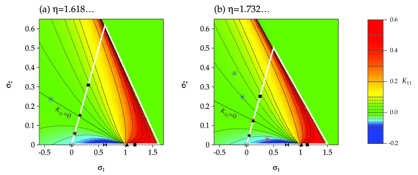
Figure 1: The triangle of the classically accessible region determined by Eq. (5) is indicated by white lines in the $(\sigma_{1},\sigma_{2})$ plane at bifurcation deformations (a) $\eta=1.618\ldots$ and (b) $\eta=\sqrt{3}$. The red and blue dots with circles indicate the 3DPO stationary points inside (really existing 3DPO) and outside (“ghost” 3DPO) of this triangle region, respectively. Several examples of the stationary points are indicated: on the $\sigma_{2}=0$ side, the short 2DPO (elliptic triangle, square, and hyperbolic “butterfly”); on the $\sigma_{2}=\sigma_{1}$ side, the short EQPO (triangle, square, star, and diameter (black crossed circle)). The long diameter (separatrix) is located at ($\sigma_{1}=1,\sigma_{2}=0$). The color and the contour curves indicate (in unit of $p\zeta/\pi$) the curvature $K_{11}$ defined by Eq. (27).

Figure 1 shows the stationary points corresponding to the 3DPO for two bifurcation points $\eta_{\rm bif}$ given by (8). The physical tori region (5) in the variables $\sigma_{i}$ is the triangle. At $\eta_{\rm bif}=1.618\ldots$ (Fig. 1a), the stationary point for the 3DPO $(5,2,1)$ coincides with that for the star-shaped $(5,2)$ orbit in the equatorial plane (discussed below) lying on the boundary with $\sigma_{2}=\sigma_{1}$, and moves toward inside of the physical tori

Figure 2: Short 3D periodic orbits (5,2,1) and (6,2,1) bifurcated from the equatorial plane orbits (5,2) and 2(3,1), respectively. Their projections on the equatorial plane are also represented by thick-dashed lines.

region for larger deformations. At $\eta_{\rm bif}=\sqrt{3}$ (Fig. 1b), the stationary point for the 3DPO $(6,2,1)$ lies at the boundary side and coincides with that for triangular orbits in the equatorial plane. At these bifurcation deformations, the lengths of the 3DPO $(5,2,1)$ and $(6,2,1)$ coincide with those of the star $(5,2)$ and the doubly repeated triangle $2(3,1)$, respectively. Figure 2 illustrates some short 3DPO, and their projections onto the equatorial plane which remind us of the parent equatorial orbits.

2.3 Orbits in the meridian plane

Equation (7) have partial solutions for $\kappa(\sigma_{1},\sigma_{2})$ and $\theta(\sigma_{1},\sigma_{2})$ which correspond to the separate families of orbits, i.e. two-dimensional periodic orbits (2DPO), in the meridian planes (containing the symmetry axis $z$) and in the equatorial plane. First, we consider the special solutions of Eq. (7) corresponding to the two-parametric (${\cal K}=2$) 2DPO families in the meridian plane.[8, 9] For these orbits, $\sigma_{2}=0$ and $\sigma_{1}$ is in the regions

$$0<\sigma_{1}<1,\qquad 1<\sigma_{1}<\frac{\eta^{2}}{\eta^{2}-1},$$ (9)

for the hyperbolic 2DPO (with hyperbolic caustics $u=\pm u_{c}$) and the elliptic 2DPO (with elliptic caustics $v=v_{c}$), respectively. The periodicity condition (7b) becomes the identity $\omega_{\varphi}/\omega_{u}\equiv 1$  ($n_{\varphi}=1$, $n_{u}=1$), and $\theta$ is fixed by

$$\theta=\theta_{h}=\arcsin\left(\frac{\sqrt{\eta^{2}-1}}{\eta}\right),\qquad\theta=\theta_{e}=\arcsin\left(\frac{\sqrt{\eta^{2}-1}}{\kappa\eta}\right),$$ (10)

for the hyperbolic and elliptic 2DPO, respectively. For $\kappa$, we only have the condition Eq. (7a). This $\kappa$ determines $\sigma_{1}$ and thus $I_{u}$ and $I_{v}$ ($I_{\varphi}=0$ since $\sigma_{2}=0$) through

$$\kappa=\kappa_{h}=\sqrt{\sigma_{1}},\qquad\kappa=\kappa_{e}=\frac{1}{\sqrt{\sigma_{1}}},$$ (11)

for the hyperbolic and elliptic orbits, respectively.

Figure 3: Some short meridian-plane orbits in the prolate spheroidal cavity: From the left to the right; the isolated long diameter $(2,1,1)$, the elliptic triangular $(3,1,1)$, the elliptic rhomboidal $(4,1,1)$, the hyperbolic “butterfly” $(4,2,1)$.

Some examples of the hyperbolic and elliptic orbits lying along the triangular boundary side $\sigma_{2}=0$ are indicated in Fig. 1; see also their geometrical illustrations in Fig. 3. The hyperbolic and elliptic tori parts are separated by the separatrix point ($\sigma_{1}=1,\sigma_{2}=0$) related to the long diameter (see below). Another end point of the hyperbolic tori coincides with the stationary point ($\sigma_{1}=\sigma_{2}=0$) for the diametric orbit in the equatorial plane. We can think of these hyperbolic and elliptic orbits as being periodic in the plane $\varphi=\mbox{const}$ and we call them “meridian-plane periodic orbits”.

For the elliptic case, the solution $\kappa$ of Eq. (7) with $\theta=\theta_{e}(\kappa)$ exists for any $n_{u}=1,2,\cdots$ and $n_{v}\geq 2n_{u}+1,(n_{\varphi}=n_{u})$ at any deformation $\eta>1$. Examples are the triangles $(n_{v}=3,n_{\varphi}=1,n_{u}=1)$, the rhomboids $(4,1,1)$ and the star-shaped orbits $(5,2,2)$ as one-parameter families in the meridian plane. The root $\kappa$ found from Eq. (7) gives the elliptic caustics with $u_{c}=\pi/2$ in Eq. (6) and the semi-axes $a_{c}=\zeta\sqrt{1-\kappa^{2}}/\kappa$ and $b_{c}=\zeta/\kappa$.

For the hyperbolic case, the solutions $\kappa$ can be found for $n_{u}=1,2,3,\cdots$ and even $n_{v}$ ($n_{v}\geq 2(n_{u}+1)$). In Fig. 1 the “butterfly” orbit $(4,2,1)$ is indicated as an example. The families of these orbits appear for $\eta>\eta_{\rm bif}$ with

$$\eta_{\rm bif}=\left[\sin\left(\frac{\pi n_{u}}{n_{v}}\right)\right]^{-1}.$$ (12)

This is the deformation where the diametric orbits $M(2,1)$ with $M\geq 2$ in the equatorial plane bifurcate and the hyperbolic orbits emerge from them. Their hyperbolic caustics are expressed in terms of the root $\kappa$ of Eq. (7) and Eq. (6) with $v_{c}=0$. The parameters $a_{c}$ and $b_{c}$ of these caustics are given by $a_{c}=\zeta\sqrt{1-\kappa^{2}}$ and $b_{c}=\zeta\kappa$.

2.4 Orbits in the equatorial plane

In the equatorial plane with $z=0$, the separate families of regular polygons and diameters are the same as in a circular billiard[3] of radius $a$. The restriction $z=0$ decreases the number $\cal K$ to ${\cal K}=1$. This single parameter corresponds to the angle of rotation of the polygons and the diameters about the symmetry axis $z$. Figure 4 illustrates the most important (shortest) equatorial-plane periodic orbits (EQPO); the diameters $M(n_{v}=2,n_{\varphi}=1)$, triangles $M(3,1)$, squares $M(4,1)$ and star-shaped orbits $M(5,2)$. They satisfy, from inequalities (5),

$$\sigma_{1}=\sigma_{2},\qquad 0\leq\sigma_{2}\leq\frac{1}{\eta^{2}-1}.$$ (13)

Therefore their stationary points lie along the $\sigma_{2}=\sigma_{1}$ side in the triangle, as indicated in Fig. 1.

Figure 4: Some short equatorial-plane orbits: From the left to the right, the short diameter $(2,1)$, the triangular $(3,1)$, the rhomboidal $(4,1)$, and the star-shaped $(5,2)$.

The caustic parameters $u_{c}$ and $v_{c}$ for these families are defined by $u_{c}=0$ and $v_{c}=\mathop{\rm arcsinh}[a\cos(\pi n_{\varphi}/n_{v})/\zeta]$. The solutions of Eq. (7) for these orbits are $\kappa=0$ and $\theta=\arcsin\sqrt{1-\sin^{2}(\pi n_{\varphi}/n_{v})/\eta^{2}}$.

2.5 Diametric orbits along the symmetry axis

In the spheroidal cavity, there is also a diametric orbit along the $z$-axis (see Fig. 3). It is isolated (${\cal K}=0$), since we have two additional restrictions $x=0$ and $y=0$ decreasing ${\cal K}$ by one unit more than in the previous case. The solution of Eq. (7) for this orbit is $\kappa=1$ and $\theta=\arcsin(\sqrt{\eta^{2}-1}/\eta)$. Its stationary point coincides with the separatrix values ($\sigma_{1}=1,\sigma_{2}=0$) corresponding formally to the caustic parameters ($u_{c}=\pi/2,~{}v_{c}=0$); see the circle point with the vertical diameter in Fig. 1. (In Fig. 1b, it is very close to the stationary point for the elliptic orbits (3,1,1) in the meridian plane, which lies slightly on the right along the $\sigma_{2}=0$ side.)

2.6 Bifurcations

At the deformations $\eta_{\rm bif}$ given by Eq. (8), the EQPO $M(n_{v},n_{\varphi})$ bifurcate and the 3DPO or the hyperbolic 2DPO $M(n_{v},n_{\varphi},n_{u})$ emerge. We encounter the breaking-of-symmetry problem at these bifurcation points since the degeneracy (symmetry) parameter ${\cal K}$ changes there, for instance, from ${\cal K}=1$ of the EQPO to ${\cal K}=2$ of the 3DPO through them. Before the bifurcations ($\eta<\eta_{\rm bif}$), the stationary points $\sigma_{i}$ of the 3DPO and the hyperbolic 2DPO are situated outside of the triangular tori region (5), and give rise to complex $(\kappa,\theta)$ and complex caustics. Such formal orbits are called “complex” or “ghost” orbits.[5] They cross the $\sigma_{1}=\sigma_{2}$ boundary through the stationary point of the EQPO at bifurcations ($\eta=\eta_{\rm bif}$) and then moves into the triangular tori region for larger $\eta$. In Fig. 1 are also indicated the stationary points for the 3DPO lying outside the physical tori region ((6,2,1) in Fig. 1a, (7,2,1) and (8,2,1) in Fig. 1b). The equatorial diameters $M(2,1)$ correspond to the limiting case, $\sigma_{1}=\sigma_{2}=0$. They bifurcate into themselves (${\cal K}=1$) and the hyperbolic 2DPO $(2M,M,1)$ in the meridian plane (${\cal K}=2$) at the deformations given by Eq. (12).

The spherical limit is a special bifurcation point. Namely, the planar regular polygons (${\cal K}=3$) and diameters (${\cal K}=2$) bifurcate into the meridian 2DPO (${\cal K}=2$), EQPO (${\cal K}=1$) and the isolated long diameter (${\cal K}=0$) for deformations $\eta>1$. Another special point is the separatrix ($\sigma_{1}=1,\sigma_{2}=0$) related to the long diameter. Near this point the complicated 3DPO, elliptic and hyperbolic 2DPO having large values of ($n_{u},n_{v}$) and $n_{u}/n_{v}$ close to $1/2$ appear. Similar bifurcations of the 3DPO, EQPO and elliptic 2DPO appear near other boundary values of $\sigma_{i}$ in the triangular tori on its “creeping” side $\sigma_{1}=\sigma_{1}^{+}(\sigma_{2})$ where some kinds of 3D “creeping” orbits having large values of $n_{v}$ but with finite and generally different $n_{u}$ and $n_{\varphi}$ appear. This is in analogy with the “creeping” singularities discussed for the elliptic orbits in the elliptic billiard[28] near the maximum value of $\sigma_{1}$, $\sigma_{1}^{\rm(cr)}=\cosh^{2}v_{b}=\eta^{2}/(\eta^{2}-1)$, according to Eq. (81) at the right vertex in the “meridian-plane orbit” side $\sigma_{2}=0$. The 3DPO with large number of the corners $n_{v}$ and finite $n_{u}=n_{\varphi}$ approach the “creeping” elliptic orbits in the meridian plane. Another vertex corresponds to the creeping EQPO having large values of $n_{v}$ and $n_{\varphi}$ but for $n_{v}/n_{\varphi}\rightarrow 1/2$.

The bifurcation point related to an appearance of “creeping” orbits cannot be reached for any finite deformation. However, even for finite deformations like superdeformed shapes, the solutions for $\sigma_{1}$ and $\sigma_{2}$ (related to the roots $\kappa$ and $\theta$ of the periodic-orbit conditions (7)) can be close to the “creeping” values of $\sigma_{1}$ and $\sigma_{2}$ (related to their boundary values of (5)). In such cases we have to take into account such bifurcations in the trace formulas for the level density. The bifurcations of the 3D and 2D diameter-like orbits with $n_{v}/n_{u}$ close to $1/2$ near the separatrix are rather long, however, so that they are not important for the shell effects discussed below.

3 Trace formulas for the prolate spheroid

3.1 Phase-space trace formula in action-angle variables

The level density $g(\varepsilon)$ is obtained from the Green function $G(\bm{r},\bm{r}^{\prime};\varepsilon)$ by taking the imaginary part of its trace:

$$g(\varepsilon)=\sum_{n}\delta\left(\varepsilon-\varepsilon_{n}\right)=-\frac{1}{\pi}\mathop{\rm Im}\int d\bm{r}^{\prime\prime}\int d\bm{r}^{\prime}G(\bm{r}^{\prime},\bm{r}^{\prime\prime};\varepsilon)~{}\delta(\bm{r}^{\prime\prime}-\bm{r}^{\prime}),$$ (14)

where $\varepsilon_{n}$ is the single-particle energy. Following Ref. mfammsb, we apply now the Gutzwiller’s trajectory expansion for the Green function $G(\bm{r},\bm{r}^{\prime},\varepsilon)$.[1, 2, 10] After simple transformations,[28] we obtain the phase-space trace formula in the action-angle variables $(\bm{I},\bm{\Theta})$,

$$g_{\rm scl}(\varepsilon) = \frac{1}{(2\pi\hbar)^{3}}\mathop{\rm Re}\sum_{\alpha}\int d\bm{\Theta}^{\prime\prime}\int d\bm{I}^{\prime}\delta\left(\varepsilon-H\left(\bm{I}^{\prime},\bm{\Theta}^{\prime}\right)\right)$$ (15)

$$\times\exp\left[\frac{i}{\hbar}\left(S_{\alpha}\left(\bm{I}^{\prime},\bm{I}^{\prime\prime},t_{\alpha}\right)+\left(\bm{I}^{\prime\prime}-\bm{I}^{\prime}\right)\cdot\bm{\Theta}^{\prime\prime}\right)-i\frac{\pi}{2}\nu_{\alpha}\right],$$

where the sum is taken over all classical trajectories $\alpha$, $\bm{I}=\{I_{u},I_{v},I_{\varphi}\}$ are the actions for the spheroidal cavity, $\bm{\Theta}=\{\Theta_{u},\Theta_{v},\Theta_{\varphi}\}$ the conjugate angles, and $\nu_{\alpha}$ phases related with the Maslov indices.[39, 41, 42, 43] The phase-space trace formula (15) is especially useful for integrable systems since the Hamiltonian $H$ does not depend on the angle variables $\bm{\Theta}$ in this case, i.e., $H=H(\bm{I})$. The action

$$S_{\alpha}\left(\bm{I}^{\prime},\bm{I}^{\prime\prime},t_{\alpha}\right)=-\int_{\bm{I}^{\prime}}^{\bm{I}^{\prime\prime}}d\bm{I}\cdot\bm{\Theta}(\bm{I})$$ (16)

is related to the standard definition

$$S_{\alpha}\left(\bm{\Theta}^{\prime},\bm{\Theta}^{\prime\prime},\varepsilon\right)=\int_{\bm{\Theta}^{\prime}}^{\bm{\Theta}^{\prime\prime}}d\bm{\Theta}\cdot\bm{I}(\bm{\Theta})$$ (17)

by the Legendre transformation

$$S_{\alpha}(\bm{\Theta}^{\prime},\bm{\Theta}^{\prime\prime},\varepsilon)+\bm{I}^{\prime\prime}\cdot(\bm{\Theta}^{\prime}-\bm{\Theta}^{\prime\prime})=S_{\alpha}(\bm{I}^{\prime},\bm{I}^{\prime\prime},t_{\alpha})+\bm{\Theta}^{\prime\prime}\cdot(\bm{I}^{\prime\prime}-\bm{I}^{\prime}),$$ (18)

$t_{\alpha}$ being the time for classical motion along the trajectory $\alpha$. The phase $\nu_{\alpha}$ will be specified below.

3.2 Stationary phase method and classical degeneracy

It should be emphasized that even for integrable systems the trace integral (15) is more general than the Poisson-sum trace formula which is the starting point of Refs. bt76,richens,sie96 for the semiclassical derivations of the level density. These two trace formulas become identical when the phase of the exponent does not depend on the angle variables $\bm{\Theta}$. In this case, the integral over angles in (15) gives simply $(2\pi)^{n}$ where $n$ is the dimension of the system ($n=3$ for the spheroidal cavity), and the stationary condition for all angle variables are identities in the $2\pi$ interval. This is true for the most degenerate classical orbits like the elliptic and hyperbolic 2DPO in the meridian plane and the 3DPO with ${\cal K}=n-1=2$. On the other hand, for orbits with smaller degeneracy like the EQPO (${\cal K}=1$) and the isolated long diameter (${\cal K}=0$), the exponent phase strongly depends on angles and possesses a definite stationary point. Therefore, we have to integrate over such angles by the ISPM in the same way as for the bifurcations of the isolated diameters in the elliptic billiard.[28]

3.3 Stationary phase conditions

Due to the energy conserving $\delta$-function, we can exactly take the integral over $I_{v}^{\prime}$ in Eq. (15) and result in

$$g_{\rm scl}(\varepsilon) = \frac{1}{(2\pi\hbar)^{3}}\mathop{\rm Re}\sum_{\alpha}\int d\Theta_{u}^{\prime\prime}\int d\Theta_{v}^{\prime\prime}\int d\Theta_{\varphi}^{\prime\prime}\int dI_{u}^{\prime}\int dI_{\varphi}^{\prime}\frac{1}{|\omega_{v}^{\prime}|}$$ (19)

$$\times\exp\left[\frac{i}{\hbar}\left(S_{\alpha}\left(\bm{I}^{\prime},\bm{I}^{\prime\prime},t_{\alpha}\right)+\left(\bm{I}^{\prime\prime}-\bm{I}^{\prime}\right)\cdot\bm{\Theta}^{\prime\prime}\right)-i\frac{\pi}{2}\nu_{\alpha}\right].$$

The integration limits for $I_{u}$ and $I_{\varphi}$ are determined by their relations to the variables ($\sigma_{1}$, $\sigma_{2}$) and by the boundaries given by Eq. (5). One of the trajectory $\alpha_{0}$ in the sum (19) is the special one which corresponds to the smooth level density $g_{\rm TF}$ of the Thomas-Fermi model.[10] For all other trajectories, we first write down the stationary phase condition for the action variables $I_{u}^{\prime}$ and $I_{\varphi}^{\prime}$ :

$$\left(\frac{\partial S_{\alpha}(\bm{I}^{\prime},\bm{I}^{\prime\prime},t_{\alpha})}{\partial I_{u}^{\prime}}\right)^{*}-\Theta_{u}^{\prime\prime}\equiv\Theta_{u}^{\prime}-\Theta_{u}^{\prime\prime}=2\pi M_{u},$$ (20a)

$$\left(\frac{\partial S_{\alpha}(\bm{I}^{\prime},\bm{I}^{\prime\prime},t_{\alpha})}{\partial I_{\varphi}^{\prime}}\right)^{*}-\Theta_{\varphi}^{\prime\prime}\equiv\Theta_{\varphi}^{\prime}-\Theta_{\varphi}^{\prime\prime}=2\pi M_{\varphi},$$ (20b)

where $\bm{M}=(M_{u},M_{v},M_{\varphi})=M(n_{u},n_{v},n_{\varphi})$ and $M$ are integer numbers which indicate the numbers of revolution along the primitive periodic orbit $\beta$. The superscript asterisk means that we take the quantities at the stationary point $I_{u}^{\prime}=I_{u}^{*}$ and $I_{\varphi}^{\prime}=I_{\varphi}^{*}$. We next use the Legendre transformation (18). Then, the stationary phase conditions with respect to angles $(\Theta_{u},\Theta_{v},\Theta_{\varphi})$ are given by

$$\left(\frac{\partial S_{\alpha}(\bm{\Theta}^{\prime},\bm{\Theta}^{\prime\prime},\varepsilon)}{\partial\bm{\Theta}^{\prime\prime}}+\frac{\partial S_{\alpha}(\bm{\Theta}^{\prime},\bm{\Theta}^{\prime\prime},\varepsilon)}{\partial\bm{\Theta}^{\prime}}\right)^{*}\equiv\bm{I}^{\prime\prime}-\bm{I}^{\prime}=0.$$ (21)

In the following derivations we have to decide whether the stationary phase conditions (all or partially) given by Eqs. (20) and (21) are identities or equations for the specific stationary points. For this purpose we have to calculate separately the contributions from the most degenerate 3DPO, the 2DPO families in the meridian plane (${\cal K}=2$) and those from orbits with smaller degeneracy like EQPO (${\cal K}=1$) and the isolated long diameter (${\cal K}=0$). The latter two kinds of orbit are different from the former two kinds in the above mentioned decision concerning the integration over angles $\bm{\Theta}$.

3.4 Three-dimensional orbits and meridian-plane orbits

The most degenerate 3DPO and the meridian-plane (elliptic and hyperbolic) 2DPO having the same values of action occupy some 3D finite areas between the corresponding caustic surfaces specified above. In this case the stationary phase conditions (21) for the integration over all angle variables $\Theta_{u}$, $\Theta_{v}$ and $\Theta_{\varphi}$ are identities. The integrand does not depend on the angle variables and the result of the integration is $(2\pi)^{3}$. Since Eq. (21) is identically satisfied (the action does not depend on the angles like the Hamiltonian $H(\bm{I})$) we have the conservation of the action variables, $I_{u}^{\prime}=I_{u}^{\prime\prime}=I_{u}$ and $I_{\varphi}^{\prime}=I_{\varphi}^{\prime\prime}=I_{\varphi}$, along the classical trajectory $\alpha$. The integrals over all $\Theta$ in Eq. (15) yield $(2\pi)^{3}$ and we are left with the Poisson-sum trace formula,[5, 10]

$$g_{\rm scl}(\varepsilon) = \frac{1}{\hbar^{3}}\mathop{\rm Re}\sum_{\bm{M}}\int d\bm{I}\>\delta\left(\varepsilon-H(\bm{I})\right)\>\exp\left[\frac{2\pi i}{\hbar}\bm{M}\cdot\bm{I}-i\frac{\pi}{2}\nu_{\bm{M}}\right]$$ (22)

$$= \frac{1}{\hbar^{3}}\mathop{\rm Re}\sum_{\bm{M}}\int dI_{u}\int dI_{\varphi}\>\frac{1}{|\omega_{v}|}\>\exp\left[\frac{2\pi i}{\hbar}\bm{M}\cdot\bm{I}-i\frac{\pi}{2}\nu_{\bm{M}}\right].$$

It is convenient to transform the integration variables ($I_{u},I_{\varphi}$) to ($\sigma_{1},\sigma_{2}$) defined by Eq. (3),

$$g_{\rm scl}(\varepsilon)=\frac{1}{\hbar^{3}}\mathop{\rm Re}\sum_{\bm{M}}p\zeta\int_{\sigma_{2}^{-}}^{\sigma_{2}^{+}}\frac{d\sigma_{2}}{2\sqrt{\sigma_{2}}}\int_{\sigma_{1}^{-}}^{\sigma_{1}^{+}}d\sigma_{1}\>\frac{\partial I_{u}}{\partial\sigma_{1}}\>\frac{1}{|\omega_{v}|}\>\exp\left[\frac{2\pi i}{\hbar}\,\bm{M}\cdot\bm{I}-i\frac{\pi}{2}\nu_{\bm{M}}\right].$$

(23)

The integration limits are much simplified when written in terms of $\sigma_{i}^{\pm}$ ($i=1,2$) and form the triangular region shown in Figs. 1. We then integrate over $\sigma_{i}$ expanding the exponent phase about the stationary point $\sigma_{i}=\sigma_{i}^{*}$,

$$2\pi\left(\bm{M}\cdot\bm{I}\right) \equiv S_{\alpha}\left(\bm{I},\bm{I}^{\prime\prime},t_{\alpha}\right)+\left(\bm{I}^{\prime\prime}-\bm{I}\right)\cdot\bm{\Theta}^{\prime\prime}$$ (24)

$$= S_{\beta}(\varepsilon)+\frac{1}{2}\sum_{i,j}J_{ij}^{\beta}(\sigma_{i}-\sigma_{i}^{*})(\sigma_{j}-\sigma_{j}^{*})+\cdots,$$

where $S_{\beta}(\varepsilon)$ is the action along the periodic orbit $\beta$,

$$S_{\beta}(\varepsilon)=2\pi M\left[n_{u}I_{u}^{*}+n_{v}I_{v}\left(\varepsilon,I_{u}^{*},I_{\varphi}^{*}\right)+n_{\varphi}I_{\varphi}^{*}\right],$$ (25)

and $I_{v}(\varepsilon,I_{u},I_{\varphi})$ the solution of the energy conservation equation $\varepsilon=H(I_{u},I_{v},I_{\varphi})$ with respect to $I_{v}$. Here the single prime index is omitted for simplicity. The $J_{ij}^{\beta}$ is the Jacobian stability factor with respect to $\sigma_{i}$ along the energy surface,

$$J_{ij}^{\beta}=\left(\frac{\partial^{2}S_{\alpha}}{\partial\sigma_{i}\partial\sigma_{j}}\right)_{\sigma_{i}=\sigma_{i}^{*}}=2\pi Mn_{v}K_{ij}^{\beta},$$ (26)

and $K_{ij}^{\beta}$ is the $(2\times 2)$ curvature matrix of the energy surface taken at the stationary point $\sigma_{i}=\sigma_{i}^{*}$ (at the periodic orbit $\beta$),

$$K_{ij}^{\beta}=\frac{\partial^{2}I_{v}}{\partial\sigma_{i}\partial\sigma_{j}}+\frac{\omega_{u}}{\omega_{v}}\frac{\partial^{2}I_{u}}{\partial\sigma_{i}\partial\sigma_{j}}+\frac{\omega_{\varphi}}{\omega_{v}}\frac{\partial^{2}I_{\varphi}}{\partial\sigma_{i}\partial\sigma_{j}}.$$ (27)

See Appendix A for the explicit expressions of these curvatures. As we shall see below, the off-diagonal curvature $K_{12}$ is non-zero for variables $\sigma_{i}$.

Then we use the ISPM, where we keep exact finite limits for integration over $\sigma_{i}$, and we finally obtain

$$\delta g_{\mathchoice{\genfrac{\{}{\}}{0.0pt}{0}{\rm 3D}{\rm 2D}}{\genfrac{\{}{\}}{0.0pt}{1}{\rm 3D}{\rm 2D}}{\genfrac{\{}{\}}{0.0pt}{2}{\rm 3D}{\rm 2D}}{\genfrac{\{}{\}}{0.0pt}{3}{\rm 3D}{\rm 2D}}}^{(2)}(\varepsilon)=\frac{1}{\varepsilon_{0}}\mathop{\rm Re}\sum_{\beta}A_{\beta}^{(2)}\,\exp\left(ikL_{\beta}-i\frac{\pi}{2}\nu_{\beta}\right),$$ (28)

where $\varepsilon_{0}=\hbar^{2}/2mR^{2}$ ($R^{3}=a^{2}b$ due to the volume conservation condition). The sum runs over all two-parameter families of the 3DPO or the meridian-plane (elliptic and hyperbolic) 2DPO, $A^{(2)}_{\beta}$ is the amplitude for a 3DPO or a 2DPO,

$$A_{\mathchoice{\genfrac{\{}{\}}{0.0pt}{0}{\rm 3D}{\rm 2D}}{\genfrac{\{}{\}}{0.0pt}{1}{\rm 3D}{\rm 2D}}{\genfrac{\{}{\}}{0.0pt}{2}{\rm 3D}{\rm 2D}}{\genfrac{\{}{\}}{0.0pt}{3}{\rm 3D}{\rm 2D}}}^{(2)} = \frac{1}{4\,\pi}\,\frac{L_{\beta}\zeta}{(Mn_{v}R)^{2}\sqrt{\sigma_{2}^{*}\left|\det K^{\beta}\right|}}\,\left[\frac{\partial I_{u}}{\partial\sigma_{1}}\right]_{\sigma_{i}=\sigma_{i}^{*}}\mathop{\rm erf}\left({\cal Z}_{1}^{-},{\cal Z}_{1}^{+}\right)\mathop{\rm erf}\left({\cal Z}_{2}^{-},{\cal Z}_{2}^{+}\right).$$

Here, $L_{\beta}$ represents “length” of the periodic orbit $\beta$

$$L_{\beta} = \frac{2\pi Mn_{v}p}{m\omega_{v}}$$ (30)

$$= 2Mn_{v}b\sin\theta\left[{\mathrm{E}}(\theta,\kappa)-\frac{{\mathrm{F}}(\theta,\kappa)}{{\mathrm{F}}\left(\kappa\right)}\,{\mathrm{E}}\left(\kappa\right)+\cot\theta\sqrt{1-\kappa^{2}\sin^{2}\theta}\right],$$

where $\theta$ and $\kappa$ are defined by the roots of periodic-orbit equations (7) ($S_{\beta}=pL_{\beta}$ for cavities). This “length” taken at the stationary points $\sigma_{i}^{*}$  (the real positive roots of Eq. (7) through Eqs. (4) and (6)) inside the finite integration range (5) represents the true length of the corresponding periodic orbit $\beta$. For other stationary points, the “length” is nothing else than the function (30) continued analytically outside the tori determined by (5). We introduced it formally instead of $\omega_{v}$ by the equation $\omega_{v}=2\pi pMn_{v}/mL_{\beta}$ for convenience. In Eq. (LABEL:amp3d2d) we introduced also the generalized error function $\mathop{\rm erf}\left({\cal Z}^{-},{\cal Z}^{+}\right)$ of the two complex arguments ${\cal Z}^{-}$ and ${\cal Z}^{+}$,

$$\mathop{\rm erf}\left(z^{-},z^{+}\right)=\frac{2}{\sqrt{\pi}}\int_{z^{-}}^{z^{+}}dz\,e^{-z^{2}}=\mathop{\rm erf}(z^{+})-\mathop{\rm erf}(z^{-}),$$ (31)

with $\mathop{\rm erf}(z)$ being the simple error function.[46] The arguments of these error functions are given by

$${\cal Z}_{1}^{\beta\,\pm} = \sqrt{-i\pi Mn_{v}K^{\beta}_{11}/\hbar}\left(\sigma_{1}^{\pm}(\sigma_{2}^{*})-\sigma_{1}^{*}\right),$$ (32a)

$${\cal Z}_{2}^{\beta\,\pm} = \sqrt{-i\pi Mn_{v}(\det K^{\beta}/K^{\beta}_{11})/\hbar}\left(\sigma_{2}^{\pm}-\sigma_{2}^{*}\right),$$ (32b)

in terms of the finite limits $\sigma_{i}^{\pm}$ given by (5), and taken at the stationary point $\sigma_{2}=\sigma_{2}^{*}$. We note that, for the 3DPO $M(3t,t,1)$ with $t=2,3,...$, the curvature $K^{\beta}_{11}$ is zero at any deformation. For such orbits, one should use

$${\cal Z}_{1}^{\beta\,\pm} = \sqrt{-i\pi Mn_{v}(\det K^{\beta}/K^{\beta}_{22})/\hbar}\,\left(\sigma_{1}^{\pm}(\sigma_{2}^{*})-\sigma_{1}^{*}\right),$$ (33a)

$${\cal Z}_{2}^{\beta\,\pm} = \sqrt{-i\pi Mn_{v}K^{\beta}_{22}/\hbar}\,\left[\sigma_{2}^{\pm}-\sigma_{2}^{*}+\frac{K_{12}^{\beta}}{K_{22}^{\beta}}\left(\sigma_{1}^{\pm}(\sigma_{2}^{*})-\sigma_{1}^{*}\right)\right],$$ (33b)

in place of (32). The latter limits (33) are derived by transforming the integration variable $\sigma_{2}$ to $\sigma_{2}-(K_{12}/K_{22})(\sigma_{1}-\sigma_{1}^{*})$.

Let us consider the stationary points $\sigma_{i}^{*}$ far from the bifurcation points. This means that they are located far from the integration limits. Accordingly, one can transform the generalized error functions to the complex Fresnel functions with the real limits and then extend the upper limit to $\infty$ and the lower one to $-\infty$. In this way we obtain asymptotically the Berry-Tabor result of the standard POT,[5] which is identical to the extended Gutzwiller’s result[9] for the most degenerate (3D and meridian-plane) orbit families,

$$A_{\mathchoice{\genfrac{\{}{\}}{0.0pt}{0}{\rm 3D}{\rm 2D}}{\genfrac{\{}{\}}{0.0pt}{1}{\rm 3D}{\rm 2D}}{\genfrac{\{}{\}}{0.0pt}{2}{\rm 3D}{\rm 2D}}{\genfrac{\{}{\}}{0.0pt}{3}{\rm 3D}{\rm 2D}}}^{(2)}(\varepsilon)=\frac{1}{\pi}\,\frac{L_{\beta}\zeta}{(Mn_{v}R)^{2}\sqrt{\sigma_{2}^{*}|\det K^{\beta}|}}\,\left[\frac{\partial I_{u}}{\partial\sigma_{1}}\right]_{\sigma_{i}=\sigma_{i}^{*}}.$$ (34)

The constant part of the phase $\nu_{\beta}$ in Eq. (28), which is independent of $\eta$ and $\varepsilon$, can be found by making use of the above asymptotic expression and applying the Maslov-Fedoryuk theory.[39, 41, 42, 43] This theory relates the Maslov index $\mu_{\beta}$ with the number of turning and caustic points for the orbit family $\beta$. For the 3DPO, the total asymptotic phase $\nu_{\beta}$ is given by

$$\nu_{\rm 3D}=\mu_{\rm 3D}-\frac{1}{2}\epsilon_{\rm 3D}+2(Mn_{u}-1),\quad\mu_{\rm 3D}=M(3n_{v}+2n_{u}).$$ (35)

Here $\mu_{\beta}$ denotes the Maslov index, the numbers of caustic and turning points traversed by the orbit. $\epsilon_{\beta}$ represents the difference of the numbers of positive and negative eigenvalues of curvature $K^{\beta}$. For the hyperbolic and elliptic meridian 2DPO, one obtains

$$\nu_{\rm 2DH}=\mu_{\rm 2DH}-\frac{1}{2}\epsilon_{\rm 2DH}+2\left(Mn_{u}-1\right),\quad\mu_{\rm 2DH}=2M\left(n_{v}+n_{u}\right)$$ (36)

and

$$\nu_{\rm 2DE}=\mu_{\rm 2DE}-\frac{1}{2}\epsilon_{\rm 2DE}+2\left(Mn_{u}-1\right),\quad\mu_{\rm 2DE}=3Mn_{v}$$ (37)

respectively. Note that the total phase includes the argument of the complex amplitude (LABEL:amp3d2d), and depends on both deformation and energy.

Near the bifurcation deformations, the stationary points $\sigma_{i}^{*}$ are close to the boundary of the finite area (5). In such cases the asymptotics of the error functions are not good approximations, and we have to carry out the integration over $\sigma_{i}$ in the calculation of the error functions in Eq. (LABEL:amp3d2d) exactly within the finite limits. One should also note that the contributions from “ghost” periodic orbits are important near the bifurcation points. It makes the trace formula continuous as function of $\eta$ at all bifurcations.

When the stationary phase points $\sigma_{i}^{*}$ are close to other boundaries of the tori, one has also to take the integrals with the finite limits; for instance, near the triangular side $\sigma_{1}=\sigma_{1}^{+}(\sigma_{2})$ where we have the “creeping” points for the 3DPO inside the tori (5) and the meridian elliptic 2DPO near the end point ($\sigma_{1}=\sigma_{1}^{+}$, $\sigma_{2}=0$) with a large number of the vertices $n_{v}\rightarrow\infty$. Another sample of such special bifurcation point is the separatrix ($\sigma_{1}=1,\sigma_{2}=0$) where 3DPO and hyperbolic 2DPO have a finite limit $n_{u}/n_{v}\rightarrow 1/2$ for $n_{v}\rightarrow\infty$ and $n_{u}\rightarrow\infty$. In this case the curvature $K_{11}$ becomes infinite and the amplitude (LABEL:amp3d2d) approaches zero. Thus, to improve the trace formula near the bifurcations, we have to evaluate the generalized error integral $\mathop{\rm erf}({\cal Z}_{i}^{\beta\,-},{\cal Z}_{i}^{\beta\,+})$ (or corresponding complex Fresnel functions[46]) in Eq. (LABEL:amp3d2d) within the finite limits ${\cal Z}_{i}^{\beta\,\pm}$ given by Eqs. (32) or (33).

For the spheroidal cavity we have another bifurcation at the spherical limit where the “azimuthal” Jacobian $J_{22}^{\beta}$ and $J_{12}^{\beta}$ (26) ($\sigma_{2}\propto I_{\varphi}^{2}$) vanishes.[9] This is the reason for the divergence of the standard POT result (34) in the spherical limit. Our improved trace formula (LABEL:amp3d2d) is finite in the spherical limit, because the “azimuthal” generalized error function $\mathop{\rm erf}({\cal Z}_{2}^{\beta\,-},{\cal Z}_{2}^{\beta\,+})$ is proportional to $\sqrt{J_{22}^{\beta}}$ in this limit and thus this “azimuthal” Jacobian is exactly canceled by that coming from the denominator of Eq. (LABEL:amp3d2d). Thus, as shown in Ref. mfimbrk, the elliptic 2DPO term (${\cal K}$=2) in the level density approach the spherical Balian-Bloch result for the most degenerate planar orbits with larger degeneracy (${\cal K}=3$),

$$\delta g_{\rm sph}^{(3)}(\varepsilon) = \frac{\sqrt{kR}}{\varepsilon_{0}}\sum_{t\geq 1,\,q>2t}\sin\left(\frac{2\pi t}{q}\right)\sqrt{\frac{\sin(2\pi t/q)}{q\pi}}$$ (38)

$$\times\sin{\left[2kRq\sin\left(\frac{\pi t}{q}\right)-\frac{3\pi}{2}q-(t-1)\pi-\frac{\pi}{4}\right]},$$

where $t=Mn_{u}$ and $q=Mn_{v}$. Note that Eq. (38) can be derived directly from the phase-space trace formula (15) or from the Poisson-sum trace formula, both rewritten in terms of the spherical action-angle variables.

3.5 Equatorial-plane orbits

We cannot apply the Poisson-sum trace formula (22) for equatorial-plane orbits, because, although the stationary-phase conditions for $\Theta_{\varphi}^{\prime\prime}$ and $\Theta_{v}^{\prime\prime}$ in Eq. (21) are identities, it is not the case for the angle variable $\Theta_{u}^{\prime\prime}$. We thus apply the ISPM for the integration over $\Theta_{u}^{\prime\prime}$.

Coming back to Eq. (19) we transform the phase-space trace formula to new “parallel” ($\Theta_{v}^{\prime\prime};I_{v}^{\prime}$) and “perpendicular” ($\Theta_{u}^{\prime\prime},\Theta_{\varphi}^{\prime\prime};I_{u}^{\prime},I_{\varphi}^{\prime}$) variables as explained in Appendix B for more general (integrable and non-integrable) systems. We then make the integration over the ($I_{u}^{\prime},I_{\varphi}^{\prime}$) variables in terms of the ISPM by transforming them into the $\sigma_{i}$ variables. Next, we consider the integration over the angle variable $\Theta_{u}^{\prime\prime}$ by the ISPM, as there is the isolated stationary point $\Theta_{u}^{*}=0$ or integer multiple of $2\pi$. We expand the exponent phase in a power series of $\Theta_{u}^{\prime\prime}$ about $\Theta_{u}^{*}=0$,

$$S_{\alpha}\left(\bm{I},\bm{I}^{\prime\prime},t_{\alpha}\right)+\left(\bm{I}^{\prime\prime}-\bm{I}\right)\cdot\bm{\Theta}^{\prime\prime}$$ (39)

$$=pL_{\rm EQ}+\frac{1}{2}\sum_{ij}J_{ij}^{\rm EQ}(\sigma_{i}-\sigma_{i}^{*})(\sigma_{j}-\sigma_{j}^{*})+\frac{1}{2}J_{\perp}^{\rm EQ}~{}\left(\Theta_{u}^{\prime\prime}\right)^{2}+\cdots,$$

where the stationary point $\sigma_{1}^{*}=\sigma_{2}^{*}\equiv\sigma^{*}$ is given by

$$\sigma^{*}=\left(\frac{I_{\varphi}^{*}}{p\zeta}\right)^{2}=\frac{a^{2}\cos^{2}\phi}{\zeta^{2}}=\frac{\cos^{2}\phi}{\eta^{2}-1},\qquad I_{\varphi}^{*}=p\,a\cos\phi.$$ (40)

$L_{\rm EQ}$ is the length of the equatorial polygon with $n_{v}$ vertices and $M$ rotations, and is given by

$$L_{\rm EQ}=2Mn_{v}R\sin\phi,\quad\phi=\pi n_{\varphi}/n_{v}.$$ (41)

In this way one finally obtains the amplitudes $A^{(1)}_{\rm EQ}$ for EQPO,

$$\delta g_{\rm EQ}^{(1)}(\varepsilon)=\frac{1}{\varepsilon_{0}}\mathop{\rm Re}\sum_{\rm EQ}A^{(1)}_{\rm EQ}\exp\left\{i\left(kL_{\rm EQ}-\frac{\pi}{2}\nu_{\rm EQ}\right)\right\},$$ (42)

$$A_{\rm EQ}^{(1)}=\sqrt{\frac{\sin^{3}\phi}{\pi Mn_{v}kR\eta F_{z}^{\rm EQ}}}\>\mathop{\rm erf}\left({\cal Z}_{1}^{-},{\cal Z}_{1}^{+}\right)\,\mathop{\rm erf}\left({\cal Z}_{2}^{-},{\cal Z}_{2}^{+}\right)\,\mathop{\rm erf}\left({\cal Z}_{3}^{-},{\cal Z}_{3}^{+}\right),$$ (43)

see Appendix B for a detailed derivation. Here, ${\cal Z}_{i}^{\pm}$ are the limits given by Eqs. (32) or (33) for $i=1,2$, and ${\cal Z}_{3}^{-}=0,{\cal Z}_{3}^{+}={\cal Z}_{\perp}^{+}$ from Eq. (133). The latter is related to the finite limits $0\leq\Theta_{u}\leq\pi/2$ for the angle $\Theta_{u}$ in the trace integration in Eq. (19), taking into account explicitly the factor 4 due to the time-reversal and spatial symmetries.

For the total asymptotic phase $\nu_{\rm EQ}$, one finds

$$\nu_{\rm EQ}=\mu_{\rm EQ}+\frac{1}{2},\quad\mu_{\rm EQ}=3Mn_{v},$$ (44)

where $\mu_{\rm EQ}$ is the Maslov index. We calculated this phase using the Maslov-Fedoryuk theory[43] at a point asymptotically far from the bifurcations. Note that the total phase is defined as the sum of the asymptotic phase $\nu_{\rm EQ}$ and the argument of the amplitude $A_{\rm EQ}$, Eq. (43), so that it depend on $kR$ and $\eta$ through the complex arguments of the product of the error functions. In the derivations of Eq. (43) we have taken into account the off-diagonal curvature as in the previous subsection, but much smaller corrections due to the mixed derivatives of the action $S_{\alpha}$ with respect to $\Theta_{u}^{\prime\prime}$ and $\sigma_{i}$ are neglected, taking $\sigma_{i}=\sigma_{i}^{*}$ in Eq. (39).

The bifurcation points are associated with zeros of the stability factor $F_{z}^{\rm EQ}$ and given by

$$\eta_{\rm bif}=\frac{\sin\phi}{\sin\left(n\phi/M\right)},\qquad n=1,2,\cdots,M.$$ (45)

The bifurcation points most important for the superdeformed shell structure are listed in Table 1.

Table 1: Bifurcation points of some short periodic orbits.

periodic orbit	$\eta_{\rm bif}$	periodic orbit	$\eta_{\rm bif}$
(4,2,1)	$\sqrt{2}$	(6,3,1)	2
(5,2,1)	1.618…	(7,3,1)	2.247…
(6,2,1)	$\sqrt{3}$	(8,3,1)	2.414…
(7,2,1)	1.802…	(9,3,1)	2.532…
(8,2,1)	1.848…

When the stationary points are located inside the finite integration region far from the ends, we transform the error functions in Eq. (43) into the Fresnel ones and extend their arguments to $\pm\infty$, except for the case when the lower limit is exactly zero. According to the definitions of the limit, Eqs. (32) and (133), for ${\cal Z}_{i}^{\pm}$, we have asymptotically ${\cal Z}_{i}^{+}\rightarrow+\infty~{}(i=1,2,3)$, ${\cal Z}_{1}^{-}={\cal Z}_{3}^{-}\rightarrow 0$, ${\cal Z}_{2}^{-}\rightarrow 0$ for diameters and ${\cal Z}_{2}^{-}\rightarrow-\infty$ for the other EQPO. Finally, we arrive at the standard Balian-Bloch formula[3] for the amplitude $A^{(1)}_{\rm EQ}$,

$$A^{(1)}_{\rm EQ}=\frac{f_{\rm EQ}}{\sqrt{\pi kR\eta}}\,\sqrt{\frac{\sin^{3}\phi}{Mn_{v}F_{z}^{\rm EQ}}}$$ (46)

where $f_{\rm EQ}=1$ for the diameters and 2 for the other EQPO ($\mathop{\rm erf}({\cal Z}_{2}^{-},{\cal Z}_{2}^{+})\rightarrow f_{\rm EQ}$ in this limit).

As seen from Eq. (46), there is a divergence at the bifurcation points where $F_{z}^{\rm EQ}\rightarrow 0$. We emphasize that our ISPM trace formula (42) has no such divergences. Indeed, the stability factor $F_{z}^{\rm EQ}$ responsible for this divergence is canceled by $F_{z}^{\rm EQ}$ from the upper limit ${\cal Z}_{3}^{+}$, Eq. (133), of the last error function in Eq. (43), ${\cal Z}_{3}^{+}\propto\sqrt{F_{z}^{\rm EQ}}$ , and we obtain the finite result at the bifurcation point:

$$A_{\rm EQ}^{(1)}=\frac{\eta^{1/3}\sin\phi\sqrt{\eta^{2}-\sin^{2}\phi}}{\sqrt{2i(\eta^{2}-1)}Mn_{v}}\>\mathop{\rm erf}\left({\cal Z}_{1}^{-},{\cal Z}_{1}^{+}\right)\,\mathop{\rm erf}\left({\cal Z}_{2}^{-},{\cal Z}_{2}^{+}\right).$$ (47)

It is very important to note that there is a local enhancement of the amplitude (47) by a factor of order $\sqrt{kR}$  near the bifurcation point. This enhancement is associated with a change of the degeneracy parameter ${\cal K}$ by one unit locally near the bifurcation point and results from exactly carrying out one integration more than in the SSPM case. In general, any change of the degeneracy parameter ${\cal K}$ by $\Delta{\cal K}$ is accompanied by the amplitude enhancement by $(kR)^{\Delta{\cal K}/2}$ because of the $\Delta{\cal K}$ extra exact integrations. These enhancement mechanism of the amplitude obtained in the ISPM is quite general and is independent of the specific choice of the potential shapes.

We mention that a more general trace formula which can be applied also to non-integrable but axially symmetric systems can be derived from the phase-space trace formula (see Appendix B).

The contribution of the equatorial diameters in Eq. (42) for deformations far from bifurcation points reduces to the Balian-Bloch result for the spherical diameters (${\cal K}=2$),

$$\delta g_{\rm sph}^{(2)}(\varepsilon)=-\frac{1}{\varepsilon_{0}}\sum_{M}\frac{1}{2\pi M}\,\sin(4MkR).$$ (48)

The amplitude for the planar polygons in the equatorial plane vanish in the spherical limit (see Appendix B). Note that the contributions of the planar polygons in the spherical cavity, Eq. (38), are obtained as the limit of $A_{\rm 2D}^{(2)}$, Eq. (LABEL:amp3d2d), for elliptic orbits in the meridian plane.[9]

3.6 Long diametric orbits and separatrics

As mentioned in §2, the curvatures $K_{ij}^{\beta}$ become infinite near the separatrix ($\sigma_{1}=1,\sigma_{2}=0$), see Appendix C. This separatrix corresponds to the isolated long diameters (${\cal K}=0$) along the symmetry axis. Thus, for the derivation of their contributions to the trace formula, the expansion up to the second order in action-angle variables considered above fails like for the turning and caustic points in the usual phase space coordinates. However, we can apply the Maslov-Fedoryuk theory [39, 41, 42, 43] in a similar way as the calculation of the Maslov indices associated with the turning and caustic points but with the use of the action-angle variables in place of the usual phase space variables. This is similar to the derivation of the long diametric term in the elliptic billiard.[28]

Starting from the phase space trace formula (19) we note that the spheroidal separatrix problem differs from the one for the elliptic billiard [28] by the integrals over the two azimuthal variables $\Theta_{\varphi}^{\prime\prime}$ and $I_{\varphi}^{\prime}$ which are additional to the integrals over $\Theta_{u}^{\prime\prime}$ and $I_{u}^{\prime}$. We expand the phase of exponent in Eq. (19) with respect to the action $I_{\varphi}^{\prime}$ and angle $\Theta_{\varphi}^{\prime\prime}$ about the stationary points $I_{\varphi}^{*}=0$ and an arbitrary $\Theta_{\varphi}^{*}$ (for instance, $\Theta_{\varphi}^{*}=0$), and take into account the third order terms, in a similar way as for the variables $\Theta_{u}^{\prime\prime}$ and $I_{u}^{\prime}$ (see Appendix C). Note that we consider here small deviations from the long diameters, and $\Theta_{\varphi}^{*}$ determines the azimuthal angle of the final point $\bm{r}^{\prime\prime}$ of this trajectory near the symmetry axis.

After the procedure explained in Appendix C, we obtain

$$\delta g^{(0)}_{\rm LD}(\varepsilon) = \frac{\pi b}{2\varepsilon_{0}R}\mathop{\rm Re}\sum_{M}\frac{1}{kR}\>e^{ikL_{\rm LD}-i\frac{\pi}{2}\nu_{\rm LD}}\prod_{j=1}^{2}e^{\frac{2i}{3}\left[(w_{j}^{\parallel})^{3/2}+(w_{j}^{\perp})^{3/2}\right]}\frac{\left(w_{j}^{\parallel}w_{j}^{\perp}\right)^{1/4}}{\sqrt{|c_{2,j}^{\parallel}c_{2,j}^{\perp}|}}$$ (49)

$$\times[\mathop{\rm Ai}(-w_{j}^{\parallel})+i\mathop{\rm Gi}(-w_{j}^{\parallel})]$$

$$\times[\mathop{\rm Ai}(-w_{j}^{\perp},{\cal Z}_{\perp}^{-},{\cal Z}_{\perp}^{+})+i\mathop{\rm Gi}(-w_{j}^{\perp},{\cal Z}_{\perp}^{-},{\cal Z}_{\perp}^{+})]$$

(see Appendix C for notations used here).

For finite deformations and sufficiently large $kR$, i.e. for large $p\zeta\propto kR\sqrt{\eta^{2}-1}$, near the separatrix $\sigma_{1}\rightarrow 1,\sigma_{2}\rightarrow 0$, the incomplete Airy functions in this equation can be approximated by the complete ones. Thus, Eq. (49) reduces to the standard Gutzwiller’s result for the isolated diameters,[3, 9]

$$\delta g^{(0)}_{\rm LD}(\varepsilon)=\frac{2b}{\pi\varepsilon_{0}kR^{2}}\sum_{M}\frac{1}{|F_{xy}^{\rm LD}|}\cos\left[kL_{\rm LD}(M)-\frac{\pi}{2}\nu_{\rm LD}\right],$$ (50)

with the length $L_{\rm LD}(M)=4Mb=4M\eta^{2/3}R$ and the stability factor $F_{xy}^{\rm LD}$ for long diameters given by Eq. (157).

For the calculation of the asymptotic phase $\nu_{\rm LD}$ we use this asymptotic expression and calculate the Maslov indices $\mu_{\rm LD}$ by the Maslov-Fedoryuk theory,[43]

$$\nu_{\rm LD}=\mu_{\rm LD}+2,\quad\mu_{\rm LD}=4M.$$ (51)

The additional phases, dependent on deformation and energy, come from the arguments of the complex exponents and Airy functions of the complex amplitude.

In the spherical limit, both the upper and lower limits of the incomplete Airy functions in Eq. (49) approach zero and the angle integration has the finite limit $\pi/2$ (see Appendix C). With this, the other factors ensure that the amplitude for long diameters becomes zero; namely, the long diametric contribution to the level density vanishes in the spherical limit.

4 Level density, shell energy and averaging

4.1 Total level density

The total semiclassical level density improved at the bifurcations can be written as a sum over all periodic orbit families in the spheroidal cavity considered in the previous section,

$$\delta g_{\rm scl}(\varepsilon)=\delta g_{\rm 3D}^{(2)}(\varepsilon)+\delta g_{\rm 2D}^{(2)}(\varepsilon)+\delta g_{\rm EQ}^{(1)}(\varepsilon)+\delta g_{\rm LD}^{(0)}(\varepsilon)=\sum_{\beta}\delta g_{\rm scl}^{(\beta)}(\varepsilon),$$ (52)

where the first two terms represent the contributions from the most degenerate (${\cal K}=2$) families of periodic orbits, the 3DPO and the meridian-plane 2DPO, given by Eq. (28), the third term the EQPO given by Eq. (42), and the fourth term the long diameters given by Eq. (49).

4.2 Semiclassical shell energy

The shell energy $\delta E$ can be expressed in terms of the oscillating part $\delta g_{\rm scl}^{(\beta)}(\varepsilon)$ of the semiclassical level density (52) as[4, 9, 10]

$$\delta E=\sum_{\beta}\left(\frac{\hbar}{t_{\beta}}\right)^{2}\delta g_{\rm scl}^{(\beta)}(\varepsilon_{\mathrm{F}}),\qquad N=\int_{0}^{\varepsilon_{\mathrm{F}}}d\varepsilon\>g(\varepsilon).$$ (53)

Here, $t_{\beta}$ denotes the period for a particle moving with the Fermi energy $\varepsilon_{\mathrm{F}}$ along the periodic orbit $\beta$,

$$t_{\beta}=MT_{\beta}=\frac{2\pi M}{\Omega_{\beta}},$$ (54)

$T_{\beta}$ being the primitive period ($M=1$), $M$ the number of repetitions, and $\Omega_{\beta}$ the frequency. The Fermi energy $\varepsilon_{\mathrm{F}}$ is determined by the second equation of (53) where $N$ is the particle number.

In the derivation of Eq. (53) we used an expansion of the amplitudes $A_{\beta}(\varepsilon)$ about the Fermi energy $\varepsilon=\varepsilon_{\mathrm{F}}$. Although $A_{\beta}(\varepsilon)$ are oscillating functions of the energy $\varepsilon$ (or $kR$), we can apply such an expansion, because $A_{\beta}$ are much more smooth compared to the oscillations coming from the exponent function of $kL_{\beta}$. The latter oscillations are responsible for the shell structure, while the oscillations of $A_{\beta}$ merely lead to slight modulations with much smaller frequencies.

Thus, the trace formula for $\delta E$ differs from that for $\delta g$ only by a factor $({\hbar/t_{\beta}})^{2}=(\hbar^{2}k_{\mathrm{F}}/mL_{\beta})^{2}$ near the Fermi surface, i.e. longer orbits are additionally suppressed by a factor $1/L_{\beta}^{2}$. The semiclassical shell energy is therefore determined by short periodic orbits.

4.3 Average level density

For the purpose of presentation of the level density improved at the bifurcations we need to consider only an average level density, thus also avoiding the convergence problems that usually arise when one is interested in a full semiclassical quantization.

The average level density is obtained by folding the level density with a Gaussian of width $\Gamma$:

$$g_{\Gamma}(\varepsilon)=\frac{1}{\sqrt{\pi}\Gamma}\int_{-\infty}^{\infty}d\varepsilon^{\prime}\,g(\varepsilon^{\prime})\,e^{-(\frac{\varepsilon-\varepsilon^{\prime}}{\Gamma})^{2}}\quad.$$ (55)

The choice of the Gaussian form of the averaging function is immaterial and guided only by mathematical simplicity.

Applying now the averaging procedure defined above to the semiclassical level density (52), one obtains [3, 9]

$$\delta g_{\Gamma,{\rm scl}}(\varepsilon)=\sum_{\beta}\delta g_{\rm scl}^{(\beta)}(\varepsilon)\,e^{-(\frac{\Gamma MT_{\beta}}{2\hbar})^{2}}=\sum_{\beta}\delta g_{\rm scl}^{(\beta)}(\varepsilon)\,e^{-(\frac{\gamma L_{\beta}}{2R})^{2}}.$$ (56)

The latter equation is written specifically for cavity problems in terms of the orbit length $L_{\beta}$ (in units of a typical length scale $R$) and a dimensionless parameter $\gamma$,

$$\Gamma=2\gamma\sqrt{\varepsilon\varepsilon_{0}}~{},$$ (57)

where $\gamma$ is a dimensionless quantity for averaging with respect to $kR$. Thus, the averaging yields an exponential decrease of the amplitudes with increasing $L_{\beta}$ and $\gamma$. In Ref. mfimbrk, the $\gamma$ is chosen to be 0.6. In this case, all longer orbits are strongly damped and only the short periodic orbits contribute to the oscillating part of the level density. For the study of the bifurcation phenomena in the superdeformed region, we need a significantly smaller value of $\gamma$.

Finally, we can say that the higher the degeneracy of an orbit, the larger the volume occupied by the orbit family in the phase space, and the shorter its length, the more important is its contribution to the average density of states.

5 Quantum Spheroidal Cavity

5.1 Oscillating level density

We calculated the quantum spectrum by the spherical wave decomposition method[50] in which wave functions are decomposed into the spherical waves as

$$\psi_{m}(\bm{r})={\sum_{l}}^{\prime}C_{l}\,j_{l}(kr)\,Y_{lm}(\Omega).$$ (58)

Here, $m$ denotes the magnetic quantum number, and $\sum^{\prime}$ means that $l$ is summed over even(odd) numbers for positive(negative) parity states. $j_{l}$ and $Y_{lm}$ are the usual spherical Bessel function and spherical harmonics, respectively. The expansion coefficients $C_{l}$’s are determined so that the wave function (58) satisfies the Dirichlet boundary condition

$$\psi_{m}(r=R(\Omega))=0$$ (59)

or equivalently,

$$\int d\Omega Y^{*}_{lm}(\Omega)\psi_{m}(r=R(\Omega))=0,\quad^{\forall}l.$$ (60)

By inserting (58) into (60), one obtains the matrix equation

$${\sum_{l^{\prime}}}^{\prime}B_{ll^{\prime}}(k)C_{l^{\prime}}=0,\quad B_{ll^{\prime}}(k)=\int d\Omega Y^{*}_{lm}(\Omega)j_{l^{\prime}}(kR(\Omega))Y_{l^{\prime}m}(\Omega).$$ (61)

Truncating the summation $l$ by sufficiently large number $l_{c}$, one can obtain the energy eigenvalue $\varepsilon_{n}=\hbar^{2}k_{n}^{2}/2m$ by searching the roots

$$\det{B(k_{n})}=0.$$ (62)

Figure 5: Single-particle spectrum for the spheroidal cavity as a function of axis ratio $\eta$. Solid and dashed curves represent the positive and negative parity levels, respectively.

Figure 5 shows the energy level diagram for the prolate spheroidal cavity as functions of axis ratio $\eta>1$.

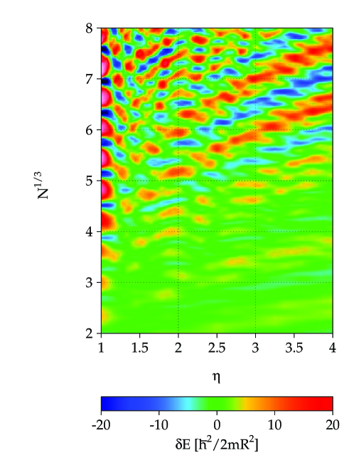
Figure 6: Shell structure energy $\delta E$ as a function of $\eta$ and $N^{1/3}$, where $N$ is the neutron (proton) number taking the spin-degeneracy factor two into account. Energies are counted in units of $\hbar^{2}/2mR^{2}~{}(\sim 30A^{-2/3}\mbox{MeV})$.

In Fig. 6, we plot shell structure energy

$$\delta E(N,\eta)=\sum_{n=1}^{N}\varepsilon_{n}(\eta)-\tilde{E}(N,\eta)$$ (63)

as functions of $\eta$ and particle number $N$. As well as the strong shell effect at the spherical shape ($\eta=1$), one clearly see a remarkable shell structure at the superdeformed shape ($\eta\sim 2$).

Next, we calculated the coarse-grained level density by the usual Strutinsky smoothing procedure by taking wave number $k$ as smoothing variable:

$$g_{\gamma}(k)=\frac{1}{\gamma}\int_{0}^{\infty}dk^{\prime}R\,f_{M}\left(\frac{kR-k^{\prime}R}{\gamma}\right)g(k^{\prime}).$$ (64)

As a smoothing function $f_{M}(x)$, we took a Gaussian with $M$-th order curvature corrections

$$f_{M}(x)=\frac{1}{\sqrt{\pi}}e^{-x^{2}}L_{M/2}^{1/2}(x^{2}),$$ (65)

where $L_{n}^{\alpha}(z)$ represents a Laguerre polynomial. Eq. (55) corresponds to the case of $M=0$. In the following, we took the order of curvature corrections $M=6$ and smoothing width $\tilde{\gamma}=2.5$ with which we can nicely satisfy the plateau condition.[44] The coarse-graining is also performed by the same smoothing function but with smaller $\gamma$. We define the oscillating part of the level density by subtracting the smooth part as

$$\delta g_{\gamma}(k)=g_{\gamma}(k)-g_{\tilde{\gamma}}(k).$$ (66)

The left-hand side of Fig. 7 shows $\delta g_{\gamma}(k)$ with $\gamma=0.3$, as functions of $\eta$ and $kR$. One will note that a remarkable shell structure emerges at $\eta\sim 2$, corresponding to the superdeformed shape.

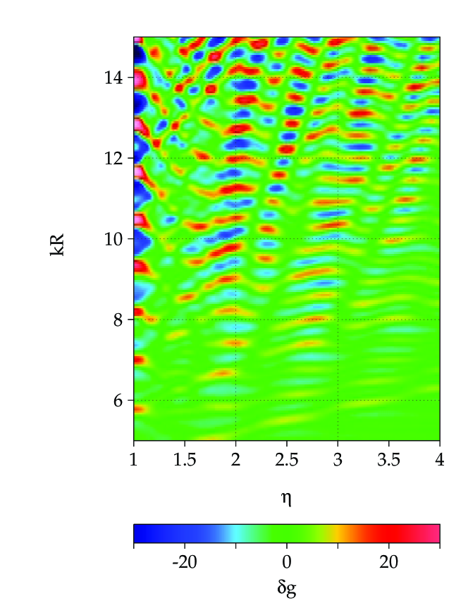
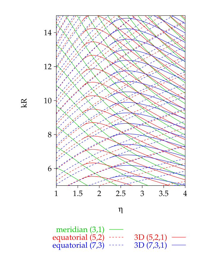
Figure 7: Oscillating part $\delta g$ of the single-particle level density as a function of $\eta$ and $kR$ (left-hand side) and stationary-action curves for several periodic orbits (right-hand side). Clear correspondence between the enhancement of the shell effect and the periodic-orbit bifurcations is seen.

Let us consider the mechanism of this strong shell effect. If a single orbit makes a dominant contribution to the periodic-orbit sum

$$\delta g_{\rm scl}(\varepsilon)=\sum_{\beta}a_{\beta}(k)\cos(kL_{\beta}-\pi\nu_{\beta}/2),\quad a_{\beta}(k)=A_{\beta}/\varepsilon_{0},$$ (67)

the major oscillating pattern in $\delta g$ should be determined by the phase factor of the dominant term. In that case, the positions of valley curves for $\delta g$ in the $(\eta,kR)$ plane are given by

$$kL_{\beta}-\pi\nu_{\beta}/2=(2n+1)\pi,\qquad(n=0,1,2,\cdots).$$ (68)

The right-hand side of Fig. 7 shows the stationary action curves (68) for several periodic orbits. Green solid curves represent the triangular orbit in the meridian plane. Other longer meridian orbits also make the same behavior but with smaller distances. Red dashed curves represent the star-shaped orbit with five vertices in the equatorial plane. It causes bifurcates at $\eta=1.618\ldots$ and the 3D orbit (5,2,1) appear (red solid curves). The sequence ($n$,2,1) ($n=5,6,7,\cdots$) make the same behavior shifting the bifurcation points a little bit to larger $\eta$. Comparing with the plot of quantum $\delta g$, one notices a clear correspondence between the superdeformed shell structure and the bifurcation of above star-shaped orbits. One will also note the correspondence between the bifurcations of the equatorial-plane orbits ($n$,3) ($n=7,8,9,\cdots$) with the hyperdeformed shell structure emerging at $\eta\simeq 2.5$. The significant shell energy gain at the superdeformed shape obtained in Fig. 6 is considered as a result of this strong shell effect in the level density.

5.2 Fourier analysis of level density

Fourier analysis is a useful tool to investigate quantum-classical correspondence in the level density.[3] Due to the simple form of action integral $S_{\beta}=\hbar kL_{\beta}$, one can easily Fourier transform the semiclassical level density $g_{\rm scl}(k)$ with respect to $k$. Let us define the Fourier transform $F(L)$ by

$$F(L)=\int dke^{-ikL}g(k).$$ (69)

In actual numerical calculations, we multiply the integrand by a Gaussian truncation function as

$$F_{\Delta}(L)=\frac{\Delta}{\sqrt{2\pi}}\int dke^{-\frac{1}{2}(k\Delta)^{2}}e^{-ikL}g(k).$$ (70)

Inserting the semiclassical level density (67), the Fourier transform is expressed as

$$F^{\rm scl}_{\Delta}(L)=\bar{F}_{\Delta}(L)+\frac{1}{2}\sum_{\beta}e^{-i\pi\nu_{\beta}/2}a_{\beta}\left(i\frac{\partial}{\partial L}\right)\exp\left[-\frac{1}{2}\left(\frac{L-L_{\beta}}{\Delta}\right)^{2}\right].$$ (71)

This is a function which has peaks at the lengths of classical periodic orbits $L=L_{\beta}$. On the other hand, we can calculate $F(L)$ by inserting the quantum mechanical level density $g(k)=\sum_{n}\delta(k-k_{n})$ as

$$F^{\rm qm}_{\Delta}(L)=\frac{\Delta}{\sqrt{2\pi}}\sum_{n}e^{-\frac{1}{2}(k_{n}\Delta)^{2}}e^{-ik_{n}L}.$$ (72)

It should present successive peaks at orbit lengths $L=L_{\beta}$. Thus we can extract information on classical periodic orbits from the quantum spectrum.

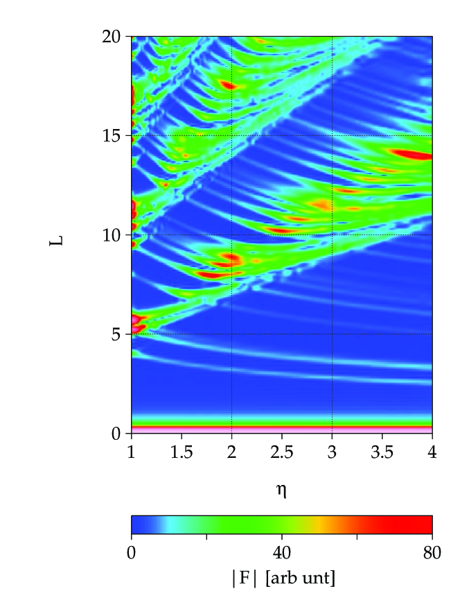
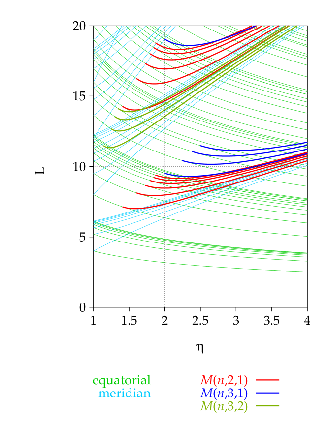
Figure 8: Fourier amplitude $|F(L)|$ of the single-particle level density (left-hand side) and lengths of classical periodic orbits (right-hand side).

In the left-hand side of Fig. 8, we plot the Fourier transform (72) as a function of $L$ and $\eta$. In the right-hand side of Fig. 8, lengths of classical periodic orbits $L_{\beta}(\eta)$ are shown. Red curves represent the orbits $M(n_{v},2,1)$ $(n_{v}=4,5,6,\cdots)$. We found strong Fourier peaks at $\eta\simeq 2$ corresponding to the periodic orbits (5,2,1), (6,2,1) and (7,2,1) just after the bifurcation points. We also found Fourier peaks at $\eta\simeq 2.5$ corresponding to the periodic orbits (7,3,1) and (8,3,1) etc. Thus, we can conclude that those periodic orbit bifurcations play essential roles in the emergence of superdeformed and hyperdeformed shell structures.

5.3 Coarse-grained shell structure energy

In order to prove that the shell structure at the superdeformed shape is due to the bifurcated orbits, we calculated the ‘coarse-grained’ shell energy defined by

$$\delta\tilde{E}_{\gamma}(N)=\int^{\tilde{k}_{\mathrm{F}}(\gamma)}\varepsilon(k)g_{\gamma}(k)dk-\int^{\tilde{k}_{\mathrm{F}}(\tilde{\gamma})}\varepsilon(k)g_{\tilde{\gamma}}(k)dk,$$ (73)

where the smoothed Fermi wave number $\tilde{k}_{\mathrm{F}}$ in each term is determined so that they satisfy the particle number condition

$$\int^{\tilde{k}_{\mathrm{F}}(\gamma)}g_{\gamma}(k)dk=\int^{\tilde{k}_{\mathrm{F}}(\tilde{\gamma})}g_{\tilde{\gamma}}(k)dk=N.$$ (74)

By coarse-graining with width $\gamma$, a shell structure of resolution $\Delta kR=\gamma$ is extracted. Classical orbits relevant for such a structure are those with lengths

$$L<L_{\rm max}=\frac{2\pi R}{\gamma}.$$ (75)

Taking $\gamma=0.6$, contributions from periodic orbits with $L\mathop{\vbox{\offinterlineskip\hbox{$>$}\hbox{$\sim$}}}10R$ are smeared out. Around the superdeformed shape, bifurcated orbits have lengths $L\sim 10R$ and those contributions are significantly weakened by smoothing with $\gamma=0.6$, and the major oscillating pattern of $\delta E$ should disappear if those bifurcated orbits are responsible for the superdeformed shell effect.

Figure 9: Shell structure energies plotted as functions of $N^{1/3}$. Solid curves represent the exact shell structure energies. Dashed and dotted curves represent those calculated by using the coarse-grained level density $g_{\gamma}(k)$ with the smoothing width $\gamma=0.3$ and $0.6$, respectively.

In Fig. 9, the coarse-grained shell energies (73) calculated for $\eta=1,2,3$, with $\gamma=0.3$ and 0.6, are compared with the exact shell structure energies. In the upper panel, one observes that the spherical shell structure survives after smoothing with $\gamma=0.6$, indicating that the major structure is determined by orbits whose lengths are sufficiently shorter than 10$R$. On the other hand, in the middle panel, one notices that the major oscillating pattern of the superdeformed shell structure is considerably broken after smoothing with $\gamma=0.6$. The same argument is valid also for $\eta=3$. This strongly supports the significance of bifurcated orbits for the superdeformed and hyperdeformed shell structures.

6 Enhancement of semiclassical amplitudes near the bifurcation points

In this section, we present some results of the semiclassical ISPM calculation, which clearly show enhancement phenomena of the semiclassical amplitudes $|A_{\rm 3D}|$ and $|A_{\rm EQ}|$ near the bifurcation points.

Figure 10: (a) Semiclassical amplitudes $|A_{\rm 3D}|$ for the 3DPO (5,2,1) and $|A_{\rm EQ}|$ for the EQPO (5,2), calculated at $kR=25$ by the ISPM, are plotted as functions of the deformation parameter $\eta$ by thick and thin solid curves, respectively. They are compared with the SSPM amplitudes (dashed curves). (b) The same as (a) but for the 3DPO (6,2,1) and the EQPO 2(3,1).

Figure 11: (a) ISPM3 amplitudes for the 3DPO (5,2,1), calculated at $kR=25$, are shown as function of deformation $\eta$ by thick-solid curves. For comparison, the ISPM amplitudes and the results of exact integration in the Poisson-sum trace formula are plotted with thin-solid and thick-dotted curves, respectively. (b) The same as (a) but for the 3DPO (6,2,1).

Figure 11a shows the modulus of the complex amplitude $A_{\rm 3D}$ (Eq. (LABEL:amp3d2d)) for the 3DPO $(5,2,1)$ and $A_{\rm EQ}$ (Eq. (43)) for the EQPO $(5,2)$ as functions of the deformation parameter $\eta$. They are compared with those of the SSPM. The SSPM amplitude for the EQPO $(5,2)$ is divergent at the bifurcation deformation $\eta_{\rm bif}=1.618\ldots$, while the ISPM amplitude is finite and continuous through this bifurcation point with a rather sharp maximum at this point. This is due to a local change of the symmetry parameter ${\cal K}$ from 1 to 2 at the bifurcation, and the associated enhancement of the amplitude is of the order $\sqrt{kR}$. As seen from Fig. 11a, the ISPM amplitude for the $(5,2,1)$ is continuous through the bifurcation point and exhibit a remarkable enhancement a little on the right of it. It approaches the SSPM amplitude given by Eq. (34) away from the bifurcation point. The ISPM enhancement for the 3DPO is also of the order $\sqrt{kR}$, because of the same change of the degeneracy parameter ${\cal K}$ from 1 to 2 as in the case of the bifurcating EQPO. The same is true for the 3DPO (6,2,1) and the EQPO 2(3,1) as shown in Fig. 11b.

In Fig. 11, we consider corrections from the 3rd-order terms in the expansion of the action about the stationary point. Here we incorporate the 3rd-order terms in the $\sigma_{1}$ variable (ISPM3) which are expected to be important for the 3DPO (6,2,1) whose curvature $K_{11}$ is identically zero (see Appendix D). We also show results of exact integration in the Poisson-sum trace formula (23) (marked POISSON). One sees that the results of the ISPM3 for the $(5,2,1)$ and $(6,2,1)$ orbits are in good agreement with those of the ISPM in the most important regions near the bifurcations and on the right-hand sides of them. It is gratifying to see that the ISPM and the ISPM3 amplitudes $|A_{\rm 3D}|$ for $(5,2,1)$ and $(6,2,1)$ are also in good agreement with the results of exact integration in the Poisson-sum trace formula. With the 3rd-order corrections, excessive ghost orbit contributions in the ISPM (bumps in the ISPM amplitudes in the left-hand side of the bifurcation point) are removed and better agreement with the result of exact integration is obtained. Except for that, the corrections due to the 3rd-order terms are rather small, and good convergence is achieved up to the second-order terms.

The amplitudes $|A_{\beta}|$ are slightly oscillating functions of $kR$. Since the period of this oscillation is much larger than that of the shell energy oscillation, one can use the expansion about the Fermi energy $\varepsilon_{\mathrm{F}}$ (or $k_{\mathrm{F}}R$) in the derivations of both the semiclassical ISPM shell energy $\delta E_{\rm scl}$ and the oscillating level density $\delta g_{\rm scl}$ (28).

Figure 12: (a) Semiclassical amplitudes $|A_{\rm 3D}|$ for the 3DPO (5,2,1) and $|A_{\rm EQ}|$ for the EQPO (5,2) are plotted by bold and thin solid curves, respectively, as functions of $kR$ at the bifurcation point $\eta=1.618\ldots$. (b) The same as (a) but for the 3DPO (6,2,1) and the EQPO 2(3,1) at the bifurcation point $\eta=1.732\ldots$. (c) Semiclassical amplitudes $|A_{\rm 3D}|$ for (5,2,1), (6,2,1) and $|A_{\rm EQ}|$ for (5,2) are plotted by thin-solid, thick-solid and dotted curves, respectively, as functions of $kR$ at $\eta=2.0$.

Figure 12 shows the semiclassical amplitudes $A_{\rm 3D}$ for the 3DPO (5,2,1) and $A_{\rm EQ}$ for the EQPO $(5,2)$ as functions of $kR$ at $\eta=1.618\ldots$ (top panel) and $\eta=2$ (bottom panel). In this figure, the semiclassical amplitudes $A_{\rm 3D}$ for the 3DPO (6,2,1) and $A_{\rm EQ}$ for the EQPO 2(3,1) are also plotted as functions of $kR$ at the bifurcation point $\eta=\sqrt{3}$ (middle panel). We see that for $\eta=2$ the amplitudes $|A_{\rm 3D}|$ for the 3DPO $(5,2,1)$ and $(6,2,1)$ become much larger than the amplitude $|A_{\rm EQ}|$ for the EQPO.

7 Comparison between quantum and semiclassical calculations

In this section we present results of calculation of level densities and shell energies with the use of the quantum Strutinsky method and the semiclassical ISPM, and make comparisons between the quantum and semiclassical calculations. In the quantum calculations, the averaging parameter $\gamma=0.3$ is used.

Figure 13: Oscillating level densities evaluated by the semiclassical ISPM, and by the quantum mechanics are shown by dotted and solid curves, respectively, as functions of $kR$ for several deformations $\eta$.

Figure 13 shows oscillating level densities $\delta g$ for relatively small deformations; QM and ISPM denote the $\delta g$ obtained by the quantum Strutinsky method and the semiclassical ISPM, respectively. For $\eta=1.2$ we obtain a good convergence of the periodic orbit sum (52) by taking into account the short elliptic 2DPO with $n_{v}\leq 12$, $n_{u}=1$, the short EQPO with the maximum vertex number $p_{\rm max}=M(n_{v})_{\rm max}=14$, and the maximum winding number $t_{\rm max}=Mn_{\varphi}=1$ ($M=1,n_{\varphi}=1$). The ISPM result is in good agreement with the quantum result. For the bifurcation point $\eta=\sqrt{2}$ of the butterfly orbit $(4,2,1)$ and $\eta=1.5$ slightly on the right of it, the convergence of the periodic-orbit sum is attained by taking into account the contributions from the bifurcating orbits, $(4,2,1)$ and the twice-repeated diameter $2(2,1)$ with $t_{\rm max}=2$, in addition to the 2DPO and the EQPO considered in the $\eta=1.2$ case.

Figure 14: The same as Fig. 13 but for larger deformations.

Figure 15: Comparison of the oscillating level densities calculated by quantum mechanics (solid curves) and those obtained by some specific semiclassical calculations (dotted curves); (a) the top panel shows a comparison with the SSPM result for $\eta=1.2$, (b) the middle panel shows the ISPM result in which only the bifurcating 3DPO $(5,2,1)$, the EQPO $(5,2)$, and the 2DPO butterfly $(4,2,1)$ are taken into account for the POT sum in Eq. (28) for $\eta=1.618\ldots$, (c) the bottom panel shows the ISPM result in which only the four shortest 3DPO are taken into account for $\eta=2.0$.

Figure 15 presents the oscillating level densities for the bifurcation deformations; $\eta=1.618\ldots$ for the EQPO $(5,2)$, $\eta=\sqrt{3}$ for the EQPO $2(3,1)$, and $\eta=2$ for the triply repeated equatorial diameters $3(2,1)$. It is interesting to compare this figure with Fig. 15 where some results of simplified semiclassical calculations are shown.

Figure 16: Semiclassical ISPM and quantum shell energies (in unit of $\varepsilon_{0}$) are plotted by dotted and solid curves, respectively, as functions of $N^{1/3}$.

Figure 17: The same as Fig. 17 but for larger deformations.

In the top panel of Fig. 15, the SSPM is used instead of the ISPM. We see that the SSPM is a good approximation for $\eta=1.2$. In the middle and bottom panels, only bifurcating orbits are taken into account in the periodic-orbit sum: only the 3DPO $(5,2,1)$, the EQPO $(5,2)$ and the butterfly $(4,2,1)$ are accounted for in the middle panel, while only the 3DPO $(5,2,1)$, $(6,2,1)$, $(7,2,1)$,$(8,2,1)$ in the bottom panel. By comparing with the corresponding ISPM results shown in Fig. 15, we see that, for $\eta=1.618\ldots$ and 2, the major patterns of the oscillation are determined by these short 3DPO.

Figures 17 and 17 show the shell energies which respectively correspond to the oscillating level densities shown in Figs. 13 and 15. Again, we see good agreement between the results of the semiclassical ISPM and the quantum calculations. For $\eta=1.2$, a good convergence is attained by including only the shortest elliptic 2DPO and EQPO, in the same way as for the level density $\delta g$, see Ref. mfimbrk. For $\eta=\sqrt{2}$ and 1.5, properties of the ISPM shell energies are similar to those considered for the elliptic billiard in Ref. mfammsb. Now, let us more closely examine the bifurcation effects in the superdeformed region by comparing Fig. 17 with Fig. 18.

Figure 18: Comparison of quantum shell energies (solid curves) with those obtained with specific semiclassical calculations (dotted curves): (a) the top panel shows the ISPM result for $\eta=1.618...$, where only the bifurcating orbits (5,2,1), (5,2) and (4,2,1) are taken into account, (b) the middle panel shows for $\eta=1.732...$ the contributions of only the three orbits; the 3DPO $(5,2,1)$ and $(6,2,1)$, and the EQPO $2(3,1)$, (c) the bottom panel shows for $\eta=2.0$ the contributions of only the four shortest 3DPO to the ISPM sum.

In the top panel of Fig. 18, we show the ISPM result for $\eta=1.618\ldots$ in which only the bifurcating 3DPO $(5,2,1)$, the short EQPO $(5,2)$ and the hyperbolic 2DPO $(4,2,1)$ are taken into account. In the middle panel of this figure, we show the ISPM shell energies at $\eta=1.732\ldots$, calculated by taking into account only the 3DPO $(5,2,1)$, the bifurcating 3DPO $(6,2,1)$ and the EQPO $2(3,1)$. These comparisons clearly indicate that a few dominant periodic orbits determine the property of quantum shell structure at those bifurcation deformations. The bottom panel in this figure shows the dominating contributions of only a few shortest 3DPO at $\eta=2.0$. Evidently, the short 3DPO $(5,2,1)$, $(6,2,1)$, $(7,2,1)$ and $(8,2,1)$ determine the major oscillating pattern of the shell energy. Thus, we can say that they are responsible for the formation of the shell structure at large deformations around the superdeformed shape. These results of calculation are in good agreement with those obtained in Ref. ask98 from the analysis of the length spectra (Fourier transforms of the quantum level densities).

8 Conclusion

We have obtained an analytical trace formula for the 3D spheroidal cavity model, which is continuous through all critical deformations where bifurcations of periodic orbits occur. We find an enhancement of the amplitudes $|A_{\beta}|$ at deformations $\eta\sim 1.6\mbox{--}2.0$ due to bifurcations of 3D orbits from the short 2D orbits in the equatorial plane. The reason of this enhancement is quite general and independent of the specific potential shapes. We believe that this is an important mechanism which contributes to the stability of superdeformed systems, also in the formation of the second minimum related to the isometric states in nuclear fission. Our semiclassical analysis may therefore lead to a deeper understanding of shell structure effects in superdeformed fermionic systems – not only in nuclei or metal clusters but also, e.g., in deformed semiconductor quantum dots whose conductance and magnetic susceptibilities are significantly modified by shell effects.

Appendix A Curvatures

A.1 Three-dimensional orbits

The action is written as

$$S=2\pi M\left(n_{v}I_{v}+n_{u}I_{u}+n_{\varphi}I_{\varphi}\right),$$ (76)

where $I_{u}$, $I_{v}$ and $I_{\varphi}$ are the partial actions. In a dimensionless form,

$$I_{u}=\frac{p\zeta}{\pi}\tilde{I}_{u},\qquad I_{v}=\frac{p\zeta}{\pi}\tilde{I}_{v},\qquad I_{\varphi}=\frac{p\zeta}{\pi}\tilde{I}_{\varphi},$$ (77)

where

$$\tilde{I}_{u} = 2\int_{0}^{z_{-}}\frac{dz}{1-z^{2}}\,\sqrt{(z^{2}-z_{-}^{2})(z^{2}-z_{+}^{2})},$$ (78a)

$$\tilde{I}_{v} = \int_{z_{+}}^{z_{b}}\frac{dz}{z^{2}-1}\,\sqrt{(z^{2}-z_{-}^{2})(z^{2}-z_{+}^{2})},$$ (78b)

$$\tilde{I}_{\varphi} = \pi\sqrt{\sigma_{2}}.$$ (78c)

$z_{\pm}$ are related to the $\sigma_{i}$ variables by

$$z_{+}^{2}+z_{-}^{2}=\sigma_{1}+1,\qquad z_{+}^{2}z_{-}^{2}=\sigma_{1}-\sigma_{2}.$$ (79)

In terms of the elliptic integrals, (78) can be expressed as

$$\tilde{I}_{u} = \frac{2}{z_{+}}\,\left[(z_{-}^{2}-1){\mathrm{F}}(k)-\sigma_{2}\mathchar 5\relax(z_{-}^{2},k)+z_{+}^{2}{\mathrm{E}}(k)\right],$$ (80a)

$$\tilde{I}_{v} = \frac{1}{z_{+}}\,\left\{(z_{+}^{2}-z_{-}^{2})\left[{\mathrm{F}}(\varphi,k)-\mathchar 5\relax(\varphi,n,k)\right]-z_{+}^{2}{\mathrm{E}}(\varphi,k)\right\}+z_{b}\sin{\varphi},$$ (80b)

with

$$k=\frac{z_{-}}{z_{+}},\qquad n=\frac{1-z_{-}^{2}}{1-z_{+}^{2}},\qquad\varphi=\arcsin\sqrt{\frac{z_{b}^{2}-z_{+}^{2}}{z_{b}^{2}-z_{-}^{2}}},$$

$$z_{b}=\cosh v_{b}=\frac{\eta}{\sqrt{\eta^{2}-1}}.$$ (81)

Here, we used the standard definitions of the elliptic integrals of the first and the third kind

$${\mathrm{F}}(\varphi,k)=\int_{0}^{\varphi}\frac{dx}{\sqrt{1-k^{2}\sin^{2}{x}}},$$ (82a)

$${\mathrm{E}}(\varphi,k)=\int_{0}^{\varphi}\sqrt{1-k^{2}\sin^{2}{x}}\>dx,$$ (82b)

$$\mathchar 5\relax(\varphi,n,k)=\int_{0}^{\varphi}\frac{dx}{(1-n\sin^{2}{x})\sqrt{1-k^{2}\sin^{2}x}}.$$ (82c)

and omit argument $\varphi=\pi/2$ for complete elliptic integrals. The action (76) is written as

$$S=2p\zeta M\left(n_{v}\tilde{I}_{v}+n_{u}\tilde{I}_{u}+n_{\varphi}\tilde{I}_{\varphi}\right).$$ (83)

The curvatures $K_{ij}$ of the energy surface $\varepsilon=H(\sigma_{1},\sigma_{2},\varepsilon)$ are defined as

$$K_{ij}=\frac{p\zeta}{\pi}\tilde{K}_{ij}=\frac{\partial^{2}I_{v}}{\partial\sigma_{i}\partial\sigma_{j}}+\frac{\omega_{u}}{\omega_{v}}\,\frac{\partial^{2}I_{u}}{\partial\sigma_{i}\partial\sigma_{j}}+\frac{\omega_{\varphi}}{\omega_{v}}\,\frac{\partial^{2}I_{\varphi}}{\partial\sigma_{i}\sigma_{j}\partial,}$$ (84)

and the frequency ratios in Eq. (84) are given by

$$\frac{\omega_{u}}{\omega_{v}}\equiv-\left(\frac{\partial I_{v}}{\partial I_{u}}\right)_{I_{\varphi}}=-\frac{\partial\tilde{I}_{v}/\partial\sigma_{1}}{\partial\tilde{I}_{u}/\partial\sigma_{1}}\,,$$ (85)

$$\frac{\omega_{\varphi}}{\omega_{v}}\equiv-\left(\frac{\partial I_{v}}{\partial I_{\varphi}}\right)_{I_{u}}=-\frac{2\sqrt{\sigma_{2}}}{\pi}\,\left[\frac{\partial\tilde{I}_{v}}{\partial\sigma_{2}}+\frac{\omega_{u}}{\omega_{v}}\frac{\partial\tilde{I}_{u}}{\partial\sigma_{2}}\right]\,.$$ (86)

We used here the properties of Jacobians for the transformations from the variables ($I_{u},I_{\varphi}$) to ($\sigma_{1},\sigma_{2}$). For the first derivatives of the actions (78) with respect to $\sigma_{1}$ and $\sigma_{2}$, one obtains

$$\frac{\partial\tilde{I}_{u}}{\partial\sigma_{1}}=\frac{1}{z_{+}}\,{\mathrm{F}}(k)\,,\qquad\frac{\partial\tilde{I}_{v}}{\partial\sigma_{1}}=-\frac{1}{2z_{+}}\,{\mathrm{F}}(\varphi,k)\,,$$ (87a)

$$\frac{\partial\tilde{I}_{u}}{\partial\sigma_{2}}=-\frac{1}{z_{+}}\,\mathchar 5\relax(z_{-}^{2},k)\,,\qquad\frac{\partial\tilde{I}_{v}}{\partial\sigma_{2}}=C_{\mathrm{F}}\,{\mathrm{F}}(\varphi,k)+C_{\mathchar 5\relax}\,\mathchar 5\relax(\varphi,n,k)\,,$$ (87b)

with

$$C_{\mathrm{F}} = \frac{z_{+}^{2}-1}{2z_{+}\sigma_{2}}=-\frac{1}{2z_{+}(z_{-}^{2}-1)}\,,$$

$$C_{\mathchar 5\relax} = -\frac{z_{+}^{2}-z_{-}^{2}}{2z_{+}\sigma_{2}}=\frac{z_{+}^{2}-z_{-}^{2}}{2z_{+}(z_{+}^{2}-1)(z_{-}^{2}-1)}\,.$$ (88)

For the second derivatives of these actions, one obtains

$$\frac{\partial^{2}\tilde{I}_{u}}{\partial\sigma_{1}^{2}} = \frac{1}{2z_{+}^{3}}\,\left\{\frac{1}{k^{2}}\left[\mathchar 5\relax(k^{2},k)-{\mathrm{F}}(k)\right]\left(\frac{\partial z_{-}^{2}}{\partial\sigma_{1}}-k^{2}\frac{\partial z_{+}^{2}}{\partial\sigma_{1}}\right)-\frac{\partial z_{+}^{2}}{\partial\sigma_{1}}{\mathrm{F}}(k)\right\}\,,$$ (89a)

$$\frac{\partial^{2}\tilde{I}_{v}}{\partial\sigma_{1}^{2}} = -\frac{1}{4z_{+}^{3}}\,\biggl{\{}\frac{1}{k^{2}}\left[\mathchar 5\relax(\varphi,k^{2},k)-{\mathrm{F}}(\varphi,k)\right]\left(\frac{\partial z_{-}^{2}}{\partial\sigma_{1}}-k^{2}\frac{\partial z_{+}^{2}}{\partial\sigma_{1}}\right)$$ (89b)

$$\hskip 135.0002pt-\frac{\partial z_{+}^{2}}{\partial\sigma_{1}}\,{\mathrm{F}}(\varphi,k)+\frac{2z_{+}^{2}}{\Delta_{\varphi}}\,\frac{\partial\varphi}{\partial\sigma_{1}}\biggr{\}},$$

$$\frac{\partial^{2}\tilde{I}_{u}}{\partial\sigma_{2}^{2}} = \frac{1}{2z_{+}^{5}k_{1}^{2}}\left[\mathchar 5\relax(z_{-}^{2},k)+2z_{+}^{2}\,\frac{\partial\mathchar 5\relax(z_{-}^{2},k)}{\partial n}+\frac{1+k^{2}}{k}\,\frac{\partial\mathchar 5\relax(z_{-}^{2},k)}{\partial k}\right],$$ (89c)

$$\frac{\partial^{2}\tilde{I}_{v}}{\partial\sigma_{2}^{2}} = \frac{\partial C_{\mathrm{F}}}{\partial\sigma_{2}}\,{\mathrm{F}}(\varphi,k)+C_{\mathrm{F}}\left(\frac{1}{\Delta_{\varphi}}\frac{\partial\varphi}{\partial\sigma_{2}}+\frac{\partial{\mathrm{F}}(\varphi,k)}{\partial k}\frac{\partial k}{\partial\sigma_{2}}\right)+\frac{\partial C_{\mathchar 5\relax}}{\partial\sigma_{2}}\,\mathchar 5\relax(\varphi,n,k)$$

$$+C_{\mathchar 5\relax}\left(\frac{\partial\mathchar 5\relax(\varphi,n,k)}{\partial\varphi}\frac{\partial\varphi}{\partial\sigma_{2}}+\frac{\partial\mathchar 5\relax(\varphi,n,k)}{\partial n}\frac{\partial n}{\partial\sigma_{2}}+\frac{\partial\mathchar 5\relax(\varphi,n,k)}{\partial k}\frac{\partial k}{\partial\sigma_{2}}\right),$$

and

$$\frac{\partial^{2}\tilde{I}_{u}}{\partial\sigma_{1}\partial\sigma_{2}} = -\frac{1}{2z_{+}^{5}k_{1}^{2}}\,\left[{\mathrm{F}}(k)+\frac{1+k^{2}}{k}\,\frac{\partial{\mathrm{F}}(k)}{\partial k}\right],$$ (89e)

$$\frac{\partial^{2}\tilde{I}_{v}}{\partial\sigma_{1}\partial\sigma_{2}} = \frac{1}{4z_{+}^{5}k_{1}^{2}}\left[{\mathrm{F}}\left(\varphi,k\right)-\frac{(\sigma_{1}+1-2z_{b}^{2})\tan\theta}{\Delta_{\varphi}z_{b}^{2}\Delta_{\theta}^{2}k_{1}}+\frac{1+k^{2}}{k}\,\frac{\partial{\mathrm{F}}(\varphi,k)}{\partial k}\right].$$

Here,

$$\Delta_{x}=\sqrt{1-k^{2}\sin^{2}x},\quad k_{1}=\sqrt{1-k^{2}},\quad\theta=\arcsin\left(\frac{z_{+}}{z_{b}}\right),$$ (90)

and

$$\frac{\partial z_{\pm}^{2}}{\partial\sigma_{1}}=\frac{1}{2}\,\left[1\pm\frac{\sigma_{1}-1}{\sqrt{(\sigma_{1}-1)^{2}+4\sigma_{2}}}\right]=\frac{1}{2}\,\left[1\pm\frac{z_{+}^{2}+z_{-}^{2}-2}{z_{+}^{2}-z_{-}^{2}}\right]\,,$$ (91)

$$\frac{\partial\varphi}{\partial\sigma_{1}}=\frac{1}{2}\,\frac{\frac{\partial z_{-}^{2}}{\partial\sigma_{1}}(z_{b}^{2}-z_{+}^{2})-\frac{\partial z_{+}^{2}}{\partial\sigma_{1}}(z_{b}^{2}-z_{-}^{2})}{(z_{b}^{2}-z_{-}^{2})\sqrt{(z_{b}^{2}-z_{+}^{2})(z_{+}^{2}-z_{-}^{2})}}\,,$$ (92)

$$\frac{\partial k^{2}}{\partial\sigma_{2}}=-\frac{1+k^{2}}{z_{+}^{4}k_{1}^{2}}\,,$$ (93)

$$\frac{\partial C_{\mathrm{F}}}{\partial\sigma_{2}} = \frac{z_{-}^{2}-2z_{+}^{2}-1}{4z_{+}^{3}(1-z_{-}^{2})^{2}(z_{+}^{2}-z_{-}^{2})},$$

$$\frac{\partial C_{\mathchar 5\relax}}{\partial\sigma_{2}} = -\frac{\sigma_{2}(3z_{+}^{2}+z_{-}^{2})-2z_{+}^{2}(z_{+}^{2}-z_{-}^{2})^{2}}{4z_{+}^{3}\sigma_{2}^{2}(z_{+}^{2}-z_{-}^{2})}\,,$$ (94)

$$\frac{\partial\varphi}{\partial\sigma_{2}}=\frac{\left(2z_{b}^{2}-(\sigma_{1}+1)\right)\tan{\theta}}{2z_{b}^{2}z_{+}^{4}k_{1}^{3}\Delta_{\theta}^{2}},$$ (95)

$$\frac{\partial n}{\partial\sigma_{2}}=\frac{\sigma_{1}-1}{(1-z_{+}^{2})^{2}(z_{+}^{2}-z_{-}^{2})},$$ (96)

$$\frac{\partial z_{\pm}^{2}}{\partial\sigma_{2}}=\pm\frac{1}{z_{+}^{2}-z_{-}^{2}}.$$ (97)

Derivatives of elliptic integrals are given by

$$\frac{\partial{\mathrm{F}}(\varphi,k)}{\partial k}=\frac{1}{k}\left[\mathchar 5\relax(\varphi,k^{2},k)-{\mathrm{F}}(\varphi,k)\right]\,,$$ (98)

$$\frac{\partial\mathchar 5\relax(\varphi,n,k)}{\partial\varphi}=\frac{1}{(1-n\sin^{2}{\varphi})\Delta_{\varphi}}\,,$$ (99)

$$\frac{\partial\mathchar 5\relax(\varphi,n,k)}{\partial n}=\frac{1}{n}\left[\mathchar 5\relax_{21}(\varphi,n,k)-\mathchar 5\relax(\varphi,n,k)\right],$$ (100)

$$\frac{\partial\mathchar 5\relax(\varphi,n,k)}{\partial k}=\frac{1}{k}\left[\mathchar 5\relax_{13}(\varphi,n,k)-\mathchar 5\relax(\varphi,n,k)\right],$$ (101)

with

$$\mathchar 5\relax_{ij}(\varphi,n,k)=\int_{0}^{\varphi}\frac{dx}{(1-n\sin^{2}{x})^{i}(1-k^{2}\sin^{2}{x})^{j/2}}\,.$$ (102)

A.2 Meridian-plane orbits

For the meridian-plane orbits for which $I_{\varphi}=0$ ($\sigma_{2}=0$), the actions $I_{u}$ and $I_{v}$ defined by Eq. (3) can be simplified. In the dimensionless form (77) one obtains for the elliptic orbits

$$\tilde{I}_{u} = 2\sqrt{\sigma}~{}{\mathrm{E}}\left(\frac{1}{\sqrt{\sigma}}\right),$$ (103a)

$$\tilde{I}_{v} = \sqrt{\sigma}\left[{\mathrm{E}}\left(\theta_{e},\frac{1}{\sqrt{\sigma}}\right)-{\mathrm{E}}\left(\frac{1}{\sqrt{\sigma}}\right)\right]+\frac{\sqrt{\eta^{2}-\sigma(\eta^{2}-1)}}{\eta\sqrt{\eta^{2}-1}}$$ (103b)

Here we used the identity [47]

$$\mathchar 5\relax(\varphi,k^{2},k)=\left[{\mathrm{E}}(\varphi,k)-k^{2}\sin{\varphi}\cos{\varphi}/\sqrt{1-k^{2}\sin^{2}{\varphi}}\right]/(1-k^{2})\,.$$ (104)

In this subsection, we omit the suffix “1” for the variable $\sigma_{1}$ for shortness. For the hyperbolic orbits,

$$\tilde{I}_{u} = 2\left[{\mathrm{E}}(\sqrt{\sigma})-(1-\sigma)~{}{\mathrm{F}}(\sqrt{\sigma})\right],$$ (105a)

$$\tilde{I}_{v} = (1-\sigma)\left[{\mathrm{F}}(\sqrt{\sigma})-{\mathrm{F}}(\theta_{h},\sqrt{\sigma})\right]+{\mathrm{E}}(\theta_{h},\sqrt{\sigma})$$ (105b)

$$\hskip 93.89409pt-{\mathrm{E}}(\sqrt{\sigma})+\frac{\sqrt{\eta^{2}-\sigma(\eta^{2}-1)}}{\eta\sqrt{\eta^{2}-1}}$$

Equations (103) and (105) may be regarded as parametric equations in terms of the parameter $\sigma$  for the energy surface of the meridian-plane orbits, $\varepsilon(\tilde{I}_{u},\tilde{I}_{v},\tilde{I}_{\varphi}=0)$, for its elliptic and hyperbolic parts, respectively.

The curvature $K_{11}$ of the energy curve for the meridian-plane orbits can be obtained by differentiating Eqs. (103) and (105) implicitly through the parameter $\sigma$. In this way one obtains Eq. (26) with the dimensionless derivatives for the elliptic orbits

$$\frac{\partial\tilde{I}_{u}}{\partial\sigma}=\frac{1}{\sqrt{\sigma}}~{}{\mathrm{F}}\left(\frac{1}{\sqrt{\sigma}}\right),$$ (106a)

$$\frac{\partial^{2}\tilde{I}_{u}}{\partial\sigma^{2}}=-\frac{1}{2\sqrt{\sigma^{3}}}~{}\mathchar 5\relax\left(\frac{1}{\sigma},\frac{1}{\sqrt{\sigma}}\right),$$ (106b)

$$\frac{\partial\tilde{I}_{v}}{\partial\sigma}=-\frac{1}{2\sqrt{\sigma}}~{}\left[{\mathrm{F}}\left(\frac{1}{\sqrt{\sigma}}\right)-{\mathrm{F}}\left(\theta_{e},\frac{1}{\sqrt{\sigma}}\right)\right],$$ (106c)

$$\frac{\partial^{2}\tilde{I}_{v}}{\partial\sigma^{2}}=\frac{1}{4\sqrt{\sigma^{3}}}~{}\left[\mathchar 5\relax\left(\frac{1}{\sigma},\frac{1}{\sqrt{\sigma}}\right)-\mathchar 5\relax\left(\theta_{e},\frac{1}{\sigma},\frac{1}{\sqrt{\sigma}}\right)+\frac{\eta\sqrt{\eta^{2}-1}}{\sqrt{1-(1-\sigma^{-1})\eta^{2}}}\right].$$ (106d)

For the hyperbolic orbits,

$$\frac{\partial\tilde{I}_{u}}{\partial\sigma}={\mathrm{F}}(\sqrt{\sigma}),$$ (107a)

$$\frac{\partial^{2}\tilde{I}_{u}}{\partial\sigma^{2}}=\frac{1}{2\sigma}~{}\left[\mathchar 5\relax(\sigma,\sqrt{\sigma})-{\mathrm{F}}(\sqrt{\sigma})\right],$$ (107b)

$$\frac{\partial\tilde{I}_{v}}{\partial\sigma}=\frac{1}{2}~{}\left[{\mathrm{F}}(\theta_{h},\sqrt{\sigma})-{\mathrm{F}}(\sqrt{\sigma})\right],$$ (107c)

$$\frac{\partial^{2}\tilde{I}_{v}}{\partial\sigma^{2}}=\frac{1}{4\sigma}~{}\left[\mathchar 5\relax(\theta_{h},\sigma,\sqrt{\sigma})-\mathchar 5\relax(\sigma,\sqrt{\sigma})z+{\mathrm{F}}(\sqrt{\sigma})-{\mathrm{F}}(\theta_{h},\sqrt{\sigma})\right].$$ (107d)

Thus, for elliptic orbits

$$\tilde{K}_{11}=\frac{1}{4\sqrt{\sigma^{3}}}\left[\frac{{\mathrm{F}}(\theta_{e},\kappa)}{{\mathrm{F}}(\kappa)}\mathchar 5\relax(\kappa^{2},\kappa)-\mathchar 5\relax(\theta_{e},\kappa^{2},\kappa)+\frac{\sqrt{\eta^{2}-\sigma(\eta^{2}-1)}}{\eta\sqrt{\eta^{2}-1}}\right],$$ (108)

and for hyperbolic orbits

$$\tilde{K}_{11}=-\frac{1}{4\sigma}\left[\frac{{\mathrm{F}}(\theta_{h},\kappa)}{{\mathrm{F}}(\kappa)}\mathchar 5\relax(\kappa^{2},\kappa)-\mathchar 5\relax(\theta_{h},\kappa^{2},\kappa)\right].$$ (109)

A.3 Equatorial-plane orbits

For the equatorial limit $\sigma_{2}=\sigma_{1}\equiv\sigma$ one obtains from (79)

$$z_{-}^{2}=0,\qquad z_{+}^{2}=\sigma+1\,.$$ (110)

We thus obtain in this limit ($k\to 0$)

$$\frac{\partial\tilde{I}_{u}}{\partial\sigma_{1}}=\frac{\pi}{2\sqrt{\sigma+1}},\qquad\frac{\partial\tilde{I}_{v}}{\partial\sigma_{1}}=-\frac{\varphi_{\rm EQ}}{2\sqrt{\sigma+1}},$$

$$\frac{\partial z_{\pm}^{2}}{\partial\sigma_{1}}=\mathchoice{\genfrac{\{}{\}}{0.0pt}{0}{\sigma/(\sigma+1)}{1/(\sigma+1)}}{\genfrac{\{}{\}}{0.0pt}{1}{\sigma/(\sigma+1)}{1/(\sigma+1)}}{\genfrac{\{}{\}}{0.0pt}{2}{\sigma/(\sigma+1)}{1/(\sigma+1)}}{\genfrac{\{}{\}}{0.0pt}{3}{\sigma/(\sigma+1)}{1/(\sigma+1)}}\,.$$ (111)

and

$$\frac{\partial^{2}\tilde{I}_{u}}{\partial\sigma_{1}^{2}} = \frac{\pi(1-2\sigma)}{8(\sigma+1)^{5/2}},$$

$$\frac{\partial^{2}\tilde{I}_{v}}{\partial\sigma_{1}^{2}} = \frac{1}{8(\sigma+1)^{5/2}}\Biggl{\{}(2\sigma-1)\varphi_{\rm EQ}+\frac{1}{2}\sin{(2\varphi_{\rm EQ})}$$

$$-\frac{2\sqrt{\sigma+1}\left[z_{b}^{2}(1-\sigma)-(\sigma+1)\right]}{z_{b}^{2}\sqrt{z_{b}^{2}-(\sigma+1)}}\Biggr{\}},$$

$$\varphi_{\rm EQ} = \arcsin\frac{\sqrt{z_{b}^{2}-(\sigma+1)}}{z_{b}}$$ (112)

Substituting (111) and (112) into (84) one finally obtains the equatorial limit

$$\tilde{K}_{11}^{\rm EQ}=\frac{z_{b}^{2}(2\sigma-1)+(\sigma+1)}{8z_{b}^{2}(\sigma+1)^{2}\sqrt{z_{b}^{2}-(\sigma+1)}}.$$ (113a)

In the same way, one obtains

$$\tilde{K}_{22}^{\rm EQ} = \frac{z_{b}^{2}(2-\sigma)+\sigma(\sigma+1)}{8z_{b}^{2}\sigma(\sigma+1)^{2}\sqrt{z_{b}^{2}-(\sigma+1)}},$$ (113b)

$$\tilde{K}_{12}^{\rm EQ} = \frac{3z_{b}^{2}-(\sigma+1)}{8z_{b}^{2}(\sigma+1)^{2}\sqrt{z_{b}^{2}-(\sigma+1)}},$$ (113c)

The determinant of the curvature matrix for EQPO becomes

$$\det\tilde{K}^{\rm EQ}=-\frac{1}{32z_{b}^{2}\sigma(\sigma+1)^{2}}$$ (114)

which is negative for any orbit and for any deformation $\eta>1$. It shows that bifurcations of EQPO’s occur only through the zeros of stability factor $F_{z}^{\rm EQ}$.

Appendix B Derivation of trace formula for the equatorial-plane orbits

We start with the phase-space trace formula[9, 28, 31, 40]

$$\delta g_{\rm scl}(\varepsilon) = \mathop{\rm Re}\sum_{\alpha}\int\frac{d\bm{q}^{\prime\prime}d\bm{p}^{\prime}}{(2\pi\hbar)^{3}}~{}\delta\left(\varepsilon-H\left(\bm{q}^{\prime},\bm{p}^{\prime}\right)\right)\left|{\cal J}\left(\bm{p}_{\perp}^{\prime\prime},\bm{p}_{\perp}^{\prime}\right)\right|^{1/2}$$ (115)

$$\times\exp\left\{\frac{i}{\hbar}\left[S_{\alpha}\left(\bm{p}^{\prime},\bm{p}^{\prime\prime},t_{\alpha}\right)+\left(\bm{p}^{\prime\prime}-\bm{p}^{\prime}\right)\cdot\bm{q}^{\prime\prime}\right]-i\frac{\pi}{2}\nu_{\alpha}\right\},$$

where the sum runs over all trajectories $\alpha$, $\bm{q}=\bm{q}_{\alpha}(t,\bm{q}^{\prime\prime},\bm{p}^{\prime})$ determined by the fixed initial momentum $\bm{p}^{\prime}$ and the final coordinate $\bm{q}^{\prime\prime}$, $H\left(\bm{q},\bm{p}\right)$ is the classical Hamiltonian, $\nu_{\alpha}$ the phase related to the Maslov index, number of caustics and turning points.[39, 41, 42, 43] The $S_{\alpha}\left(\bm{p}^{\prime},\bm{p}^{\prime\prime},t_{\alpha}\right)$ is the action in the mixed phase-space representation,

$$S_{\alpha}\left(\bm{p}^{\prime},\bm{p}^{\prime\prime},t_{\alpha}\right)=-\int_{\bm{p}^{\prime}}^{\bm{p}^{\prime\prime}}~{}d\bm{p}\cdot\bm{q}\left(\bm{p}\right),$$ (116)

related to the standard definition of the action $S_{\alpha}\left(\bm{q}^{\prime},\bm{q}^{\prime\prime},\varepsilon\right)$,

$$S_{\alpha}\left(\bm{q}^{\prime},\bm{q}^{\prime\prime},\varepsilon\right)=\int_{\bm{q}^{\prime}}^{\bm{q}^{\prime\prime}}~{}d\bm{q}\cdot\bm{p}\left(\bm{q}\right)$$ (117)

by the Legendre transformations (the integration by parts),

$$S_{\alpha}\left(\bm{p}^{\prime},\bm{p}^{\prime\prime},t_{\alpha}\right)=S_{\alpha}\left(\bm{q}^{\prime},\bm{q}^{\prime\prime},\varepsilon\right)+\left(\bm{p}^{\prime}-\bm{p}^{\prime\prime}\right)\bm{q}^{\prime\prime},$$ (118)

$t_{\alpha}$ being the time for motion of the particle along the trajectory $\alpha$. The ${\cal J}\left(\bm{p}_{\perp}^{\prime\prime},\bm{p}_{\perp}^{\prime}\right)$ in Eq. (115) is the Jacobian for the transformation from $\bm{p}_{\perp}^{\prime\prime}$ to $\bm{p}_{\perp}^{\prime}$. Here, we introduced the local system of the phase-space coordinates $\bm{q}=\left\{q_{\parallel},\bm{q}_{\perp}\right\}$ and $\bm{p}=\left\{p_{\parallel},\bm{p}_{\perp}\right\}$ splitting the vectors into the parallel and perpendicular components with respect to the trajectory $\alpha$.

For the equatorial-plane periodic orbits (EQPO) one of the perpendicular components $\bm{q}_{\perp}$ and $\bm{p}_{\perp}$ can be taken along the symmetry axis $z$, say $z$ and $p_{z}$, keeping for other perpendicular components the same suffix, $q_{\perp}$ and $p_{\perp}$. After the transformation to this local phase-space coordinate system and integration over the “parallel” momentum $p_{\parallel}=p=\sqrt{2m\varepsilon}$ by using the $\delta$-function in Eq. (115), one obtains for the contribution from the EQPO (${\cal K}=1$)

$$\delta g_{\rm EQ}^{(1)}(\varepsilon) = \frac{1}{(2\pi\hbar)^{3}}\mathop{\rm Re}\sum_{\alpha}\int\frac{dq_{\parallel}^{\prime\prime}}{|\dot{q}_{\parallel}^{\prime\prime}|}\int dq_{\perp}^{\prime\prime}dp_{\perp}^{\prime}\int dz^{\prime\prime}dp_{z}^{\prime}\left|{\cal J}\left(\bm{p}^{\prime\prime},\bm{p}^{\prime}\right)\right|^{1/2}$$ (119)

$$\times\exp\left\{\frac{i}{\hbar}\left[S_{\alpha}\left(\bm{p}^{\prime},\bm{p}^{\prime\prime},t_{\alpha}\right)+\left(\bm{p}^{\prime\prime}-\bm{p}^{\prime}\right)\cdot\bm{q}^{\prime\prime}\right]-i\frac{\pi}{2}\nu_{\alpha}\right\},$$

where $\dot{q}_{\parallel}=\partial H/\partial p_{\parallel}=p/m$ is the velocity. In the spheroidal action-angle variables, $q_{\parallel}=\Theta_{v}$, $p_{\parallel}=I_{v}$, $\dot{q}_{\parallel}=\omega_{v}$, $q_{\perp}=\Theta_{\varphi}=\varphi$, $p_{\perp}=I_{\varphi}$, $z=\Theta_{u}$, $p_{z}=I_{u}$, and we have

$$\delta g_{\rm EQ}^{(1)}(\varepsilon) = \frac{1}{(2\pi\hbar)^{3}}\mathop{\rm Re}\sum_{\alpha}\int\frac{d\Theta_{v}^{\prime\prime}}{|\omega_{v}|}\int d\Theta_{\varphi}^{\prime\prime}\,dI_{\varphi}^{\prime}\int d\Theta_{u}^{\prime\prime}\,dI_{u}^{\prime}\left|{\cal J}\left(I_{\varphi}^{\prime\prime}I_{u}^{\prime\prime},I_{\varphi}^{\prime}I_{u}^{\prime}\right)\right|^{1/2}$$ (120)

$$\times\exp\left\{\frac{i}{\hbar}\left[S_{\alpha}\left(\bm{I}^{\prime},\bm{I}^{\prime\prime},t_{\alpha}\right)+\left(\bm{I}^{\prime\prime}-\bm{I}^{\prime}\right)\cdot\bm{\Theta}^{\prime\prime}\right]-i\frac{\pi}{2}\nu_{\alpha}\right\},$$

We now perform the integrations using the expansion of the action $S_{\alpha}$ about the stationary points

$$S_{\alpha}\left(\bm{I}^{\prime},\bm{I}^{\prime\prime},t_{\alpha}\right)+\left(\bm{I}^{\prime\prime}-\bm{I}^{\prime}\right)\cdot\bm{\Theta}^{\prime\prime}$$ (121)

$$=S_{\beta}(\varepsilon)+\frac{1}{2}\sum_{ij}J_{ij}(\sigma_{i}-\sigma_{i}^{*})(\sigma_{j}-\sigma_{j}^{*})+\frac{1}{2}J_{\perp}\left(z-z^{*}\right)^{2}+\cdots$$

Here we omit the corrections associated with mixed derivatives of type $\partial^{2}S/\partial\Theta\partial I$ for simplicity. $J_{\perp}$ is the Jacobian corresponding to the second variation of the action $S_{\alpha}$ with respect to the angle variable $\Theta_{u}$,

$$J_{\perp}^{\rm EQ}=\left(\frac{\partial^{2}S_{\alpha}}{\partial{\Theta_{u}^{\prime}}^{2}}+2\frac{\partial^{2}S_{\alpha}}{\partial\Theta_{u}^{\prime}\partial\Theta_{u}^{\prime\prime}}+\frac{\partial^{2}S_{\alpha}}{\partial{\Theta_{u}^{\prime}}^{2}}\right)_{\rm EQ}=\left(-\frac{\partial I_{u}^{\prime}}{\partial\Theta_{u}^{\prime}}-2\frac{\partial I_{u}^{\prime}}{\partial\Theta_{u}^{\prime\prime}}+\frac{\partial I_{u}^{\prime\prime}}{\partial\Theta_{u}^{\prime\prime}}\right)_{\rm EQ}.$$

(122)

This quantity can be expressed in terms of the curvatures $K^{\rm EQ}$ and the Gutzwiller’s stability factor $F_{z}^{\rm EQ}$,

$$F_{z}^{\rm EQ} = -\left[\left(-\frac{\partial I_{u}^{\prime}}{\partial\Theta_{u}^{\prime}}-2\frac{\partial I_{u}^{\prime}}{\partial\Theta_{u}^{\prime\prime}}+\frac{\partial I_{u}^{\prime\prime}}{\partial\Theta_{u}^{\prime\prime}}\right)\Big{/}\frac{\partial I_{u}^{\prime}}{\partial\Theta_{u}^{\prime\prime}}\right]_{\rm EQ}$$ (123)

$$= 4\sin^{2}\left[\frac{1}{2}Mn_{v}\arccos\left(1-2\eta^{-2}\sin^{2}\phi\right)\right],$$

as

$$J_{\perp}^{\rm EQ}=-\frac{F_{z}^{\rm EQ}}{(J_{u}-J_{u\varphi}^{2}/J_{\varphi})^{\rm EQ}}=-\frac{F_{z}^{\rm EQ}}{2\pi Mn_{v}(K_{u}-K_{u\varphi}^{2}/K_{\varphi})^{\rm EQ}}$$ (124)

In these equations we used simple identical Jacobian transformations

$$\left(\frac{\partial I_{u}^{\prime}}{\partial\Theta_{u}^{\prime\prime}}\right)_{I_{\varphi}^{\prime}}^{-1} = \frac{\partial(\Theta_{u}^{\prime\prime},I_{\varphi}^{\prime})}{\partial(I_{u}^{\prime},I_{\varphi}^{\prime})}=\frac{\partial\Theta_{u}^{\prime\prime}}{\partial I_{u}^{\prime}}-\frac{\partial\Theta_{u}^{\prime\prime}}{\partial I_{\varphi}^{\prime}}\,\frac{\partial I_{\varphi}^{\prime}}{\partial I_{u}^{\prime}}=J_{u}-J_{u\varphi}\frac{J_{u\varphi}}{J_{\varphi}}$$

The curvature $K_{u}^{\rm EQ}$ is the quantity $K_{u}$ defined in (127), evaluated at stationary point $\sigma_{1}=\sigma_{2}=\sigma^{*}$ given by Eq. (40), and so on.

The integrand of (120) does not depend on the angles ($\Theta_{v}$, $\Theta_{\varphi}$) and we obtain simply $(2\pi)^{2}$ for the integration over these angle variables. We transform integration variables $(I_{u},I_{\varphi})$ into $(\sigma_{1},\sigma_{2})$ to obtain simple integration limits, and integrate over $(\sigma_{1},\sigma_{2})$ by the ISPM. In this way we obtain

$$\delta g_{\rm EQ}^{(1)}(\varepsilon) = \sqrt{\frac{\pi}{2\hbar^{3}}}\mathop{\rm Re}\sum_{\beta}e^{i(kL_{\beta}-\pi\nu_{\beta}/2)}\frac{1}{\omega_{v}}\left|\frac{\partial(I_{u},I_{\varphi})}{\partial(\sigma_{1},\sigma_{2})}\right|\sqrt{\frac{1}{J_{\perp}|\det J^{\rm EQ}|}}$$ (125)

$$\times\mathop{\rm erf}({\cal Z}_{\perp}^{-},{\cal Z}_{\perp}^{+};{\cal Z}_{1}^{-},{\cal Z}_{1}^{+};{\cal Z}_{2}^{-},{\cal Z}_{2}^{+})$$

where

$$\mathop{\rm erf}\left(x^{-},x^{+};y^{-},y^{+};z^{-},z^{+}\right)=\left(\frac{2}{\sqrt{\pi}}\right)^{3}\int_{x^{-}}^{x^{+}}dx\int_{y^{-}}^{y^{+}}dy\int_{z^{-}}^{z^{+}}dz\,e^{-x^{2}-y^{2}-z^{2}},$$

(126)

Note that the integration limits for the internal integrals over $y$ and $z$ in $\mathop{\rm erf}\left(x^{-},x^{+};y^{-},y^{+};z^{-},z^{+}\right)$ in general depend on the variable of the next integrations, $y^{\pm}=y^{\pm}(x)$ and $z^{\pm}=z^{\pm}(x,y)$. Here we define curvatures in the $(I_{u},I_{\varphi})$ variables as

$$J_{u}=\frac{\partial^{2}S_{\alpha}}{\partial I_{u}^{2}}=2\pi Mn_{v}K_{u},\quad J_{\varphi}=\frac{\partial^{2}S_{\alpha}}{\partial I_{\varphi}^{2}}=2\pi Mn_{v}K_{\varphi},$$

$$J_{u\varphi}=\frac{\partial^{2}S_{\alpha}}{\partial I_{u}\partial I_{\varphi}}=2\pi Mn_{v}K_{u\varphi}.$$ (127)

Using (124) and relations

$$\det J\equiv J_{11}J_{22}-{J_{12}}^{2}=\left|\frac{\partial(I_{u},I_{\varphi})}{\partial(\sigma_{1},\sigma_{2})}\right|^{2}(J_{u}J_{\varphi}-{J_{u\varphi}}^{2}),$$ (128)

$$K_{\varphi}=\frac{1}{\pi pa\sin\phi},\qquad\omega_{v}=\frac{\pi p}{ma\sin\phi},$$ (129)

one finally obtains

$$\delta g_{\rm EQ}^{(1)}(\varepsilon)=\frac{1}{\varepsilon_{0}}\mathop{\rm Re}\sum_{\rm EQ}~{}A_{\rm EQ}\exp\left(ikL_{\rm EQ}-i\frac{\pi}{2}\nu_{\rm EQ}\right),$$ (130)

$$A_{\rm EQ}=\frac{1}{2}\sqrt{\frac{\sin^{3}\phi}{\pi Mn_{v}kR\eta F_{z}}}\mathop{\rm erf}\left({\cal Z}_{\perp}^{-},{\cal Z}_{\perp}^{+};{\cal Z}_{1}^{-},{\cal Z}_{1}^{+};{\cal Z}_{2}^{-},{\cal Z}_{2}^{+}\right),$$ (131)

where $L_{\rm EQ}$ represents length of the EQPO. The “triple” error function in Eq. (131) can be separated into the product of three standard error functions,

$$\mathop{\rm erf}\left({\cal Z}_{\perp}^{-},{\cal Z}_{\perp}^{+};{\cal Z}_{1}^{-},{\cal Z}_{1}^{+};{\cal Z}_{2}^{-},{\cal Z}_{2}^{+}\right)\approx\mathop{\rm erf}\left({\cal Z}_{\perp}^{-},{\cal Z}_{\perp}^{+}\right)\mathop{\rm erf}\left({\cal Z}_{1}^{-},{\cal Z}_{1}^{+}\right)\mathop{\rm erf}\left({\cal Z}_{2}^{-},{\cal Z}_{2}^{+}\right)$$

(132)

by taking the limits at the stationary points for all deformations, except for a small region near the spherical shape. In this way we obtain the simple results (43). The arguments of the error functions are given by (32) or (33) for ${\cal Z}_{i}^{\pm}$ ($i=1,2$) and

$${\cal Z}_{\perp}^{\pm}=\pm\frac{\pi}{2}\sqrt{-\frac{iJ_{\perp}^{\rm EQ}}{2\hbar}}=\pm\frac{\hbar(k\zeta)^{2}}{16}\sqrt{\frac{iF_{z}^{\rm EQ}}{Mn_{v}ka\sin\phi\,\sigma^{*}(\sigma^{*}+1)\det K^{\rm EQ}}}.$$ (133)

The spherical limit is easily obtained by using the spherical action-angle variables $\{\Theta_{\theta},\Theta_{r},\Theta_{\varphi};I_{\theta},I_{r},I_{\varphi}\}$. In these variables

$$A_{\rm EQ}=\frac{1}{2}\sqrt{\frac{\sin^{3}\phi}{\pi Mn_{r}kR\eta F_{z}}}\,\mathop{\rm erf}\left({\cal Z}_{\perp}^{-},{\cal Z}_{\perp}^{+};{\cal Z}_{\theta}^{-},{\cal Z}_{\theta}^{+};{\cal Z}_{\varphi}^{-},{\cal Z}_{\varphi}^{+}\right),$$ (134)

where $n_{r}\equiv n_{v}$ for the equatorial-plane orbits with ($n_{v},n_{\varphi}$), the invariant stability factor $F_{\theta}\equiv F_{z}^{\rm EQ}$ given by (123),

$${\cal Z}_{\perp}^{\pm}=\sqrt{\frac{-i\pi F_{\theta}^{\rm EQ}}{16Mn_{r}\hbar K_{\theta}^{\rm EQ}}}(z^{\pm}-z^{*}),\quad{\cal Z}_{\mathchoice{\genfrac{\{}{\}}{0.0pt}{0}{\theta}{\varphi}}{\genfrac{\{}{\}}{0.0pt}{1}{\theta}{\varphi}}{\genfrac{\{}{\}}{0.0pt}{2}{\theta}{\varphi}}{\genfrac{\{}{\}}{0.0pt}{3}{\theta}{\varphi}}}^{\pm}=\sqrt{-i\pi Mn_{r}K_{\mathchoice{\genfrac{\{}{\}}{0.0pt}{0}{\theta}{\varphi}}{\genfrac{\{}{\}}{0.0pt}{1}{\theta}{\varphi}}{\genfrac{\{}{\}}{0.0pt}{2}{\theta}{\varphi}}{\genfrac{\{}{\}}{0.0pt}{3}{\theta}{\varphi}}}^{\rm EQ}/\hbar}\left(I_{\mathchoice{\genfrac{\{}{\}}{0.0pt}{0}{\theta}{\varphi}}{\genfrac{\{}{\}}{0.0pt}{1}{\theta}{\varphi}}{\genfrac{\{}{\}}{0.0pt}{2}{\theta}{\varphi}}{\genfrac{\{}{\}}{0.0pt}{3}{\theta}{\varphi}}}^{\pm}-I_{\mathchoice{\genfrac{\{}{\}}{0.0pt}{0}{\theta}{\varphi}}{\genfrac{\{}{\}}{0.0pt}{1}{\theta}{\varphi}}{\genfrac{\{}{\}}{0.0pt}{2}{\theta}{\varphi}}{\genfrac{\{}{\}}{0.0pt}{3}{\theta}{\varphi}}}^{*}\right).$$

(135)

The quantities $K_{\theta}^{\rm EQ}$ and $K_{\varphi}^{\rm EQ}$

$$K_{\mathchoice{\genfrac{\{}{\}}{0.0pt}{0}{\theta}{\varphi}}{\genfrac{\{}{\}}{0.0pt}{1}{\theta}{\varphi}}{\genfrac{\{}{\}}{0.0pt}{2}{\theta}{\varphi}}{\genfrac{\{}{\}}{0.0pt}{3}{\theta}{\varphi}}}^{\rm EQ}=\left(\frac{\partial^{2}I_{r}}{\partial I_{\mathchoice{\genfrac{\{}{\}}{0.0pt}{0}{\theta}{\varphi}}{\genfrac{\{}{\}}{0.0pt}{1}{\theta}{\varphi}}{\genfrac{\{}{\}}{0.0pt}{2}{\theta}{\varphi}}{\genfrac{\{}{\}}{0.0pt}{3}{\theta}{\varphi}}}^{2}}\right)_{\rm EQ}\,,\qquad$$ (136)

are the curvatures of the energy surface $\varepsilon=H(I_{\theta},I_{r},I_{\varphi})$ in the spherical coordinate system. In that system the maximum value of $I_{\varphi}$ is equal to the absolute value of the classical angular momentum $I_{\theta}$, $I_{\varphi}^{\pm}=\pm I_{\theta}$, $I_{\theta}^{+}$ being the maximum value of $|I_{\theta}|$, and $I_{\theta}^{-}=0$. We note that for the diametric orbits the stationary points $I_{\theta}^{*}$ and $I_{\varphi}^{*}$ are exactly zero and there are also specific integration limits in Eq. (134). In this case the internal integral over $I_{\varphi}$ within a small region can be evaluated approximately as $2I_{\theta}$, and one obtains for the “triple” error function

$$\mathop{\rm erf}\left({\cal Z}_{\perp}^{-},{\cal Z}_{\perp}^{+};{\cal Z}_{\theta}^{-},{\cal Z}_{\theta}^{+};{\cal Z}_{\varphi}^{-},{\cal Z}_{\varphi}^{+}\right)\rightarrow\sqrt{\frac{-4iF_{z}}{M\pi^{2}n_{r}\hbar K_{\theta}^{\rm EQ}}}=\sqrt{\frac{-4iF_{z}kR}{2\pi M}}.$$ (137)

We used here the fact that, in the spherical limit $F_{z}\rightarrow 0$, the integral over ${\cal Z}_{\theta}$ can be approximated by the upper limit ${\cal Z}_{\theta}^{+}$ given by Eq. (135). We omitted also the strong oscillating value of $\int dz^{2}e^{-z^{2}}$ at the upper limit since it vanishes after any small averaging over $kR$ and equals 1 in this approximation. We also accounted for the fact that $K_{\theta}^{\rm EQ}\rightarrow{1/(\pi pR)}$ for the diameters; see Eq. (136) ($\phi=\pi/2$ for the diameters). Finally, the stability factor $F_{z}$ is canceled and one obtains the Balian-Bloch result (46) for the contribution of the diametric orbits in the spherical cavity.[3]

For all other EQPO one has the stationary points $I_{\varphi}^{*}=I_{\theta}^{*}\neq 0$ and $I_{\varphi}$ is identical to its maximum value $I_{\theta}$ in the spherical limit. This is the reason why there is no next order ($1/\sqrt{kR}$) corrections to the Balian-Bloch trace formula for the contribution of the planar orbits with $n_{r}\geq 3$. The latter comes from the spherical limit of the elliptic orbits in the meridian plane (LABEL:amp3d2d), see Ref. mfimbrk.

Appendix C Separatrix

Like for the case of the turning points, [39, 41, 42, 43] we first expand the exponent phase in Eq. (19) with respect to $I_{u}^{\prime}$ :

$$S_{\alpha}\left(\bm{I}^{\prime},\bm{I}^{\prime\prime},t_{\alpha}\right)-\left(\bm{I}^{\prime\prime}-\bm{I}^{\prime}\right)\cdot\bm{\Theta}^{\prime\prime} = c_{0}^{\parallel}+c_{1}^{\parallel}x+c_{2}^{\parallel}x^{2}+c_{3}^{\parallel}x^{3}+\ldots$$ (138)

$$\equiv \tau_{0}^{\parallel}+\tau_{1}^{\parallel}z+\frac{1}{3}z^{3}.$$

Here

$$x=\frac{1}{\hbar}\left(I_{u}^{\prime}-{I_{u}^{\prime}}^{*}\right),$$ (139)

$$c_{0}^{\parallel}=\frac{1}{\hbar}\left[S_{\alpha}^{*}\left(\bm{I}^{\prime},\bm{I}^{\prime\prime},\varepsilon\right)-\left(\bm{I}^{\prime}-\bm{I}^{\prime\prime}\right)^{*}\cdot{\bm{\Theta}^{\prime\prime}}^{*}\right]=\frac{1}{\hbar}S_{\alpha}^{*}\left(\bm{\Theta}^{\prime},\bm{\Theta}^{\prime\prime},\varepsilon\right),$$ (140)

$$c_{1}^{\parallel}=\left(\frac{\partial S_{\alpha}}{\partial I_{u}^{\prime}}-\Theta_{u}^{\prime\prime}\right)^{*}=\Theta_{u}^{\prime}-\Theta_{u}^{\prime\prime}\rightarrow 0,\qquad\sigma_{1}\rightarrow 1,$$ (141)

$$c_{2}^{\parallel}=\frac{\hbar}{2}\left(\frac{\partial^{2}S_{\alpha}}{\partial{I_{u}^{\prime}}^{2}}\right)^{*}=2p\zeta M\hbar\tilde{K}_{u}^{\alpha}\rightarrow\infty,\qquad\sigma_{1}\rightarrow 1,$$ (142)

$$c_{3}^{\parallel}=\frac{\hbar^{3}}{6}\left(\frac{\partial^{3}S_{\alpha}}{\partial{I_{u}^{\prime}}^{3}}\right)^{*}=\frac{2\pi^{3}\hbar^{2}M}{3(p\zeta^{2})^{2}}\left(\frac{\partial\tilde{K}_{u}^{\alpha}}{\partial\tilde{I}_{u}}\right)<0,\quad\sigma_{\parallel}\rightarrow 1,$$ (143)

where the superscript asterisk indicates the value at $I_{u}^{\prime}=I_{u}^{\prime\prime}=I_{u}^{*}$. The asymptotic behavior of the constants $c_{i}^{\parallel}$ near the separatrix $\sigma_{1}\approx 1$ is found from

$$\tilde{K}_{u}^{\alpha}\rightarrow\frac{\log\left[(1+\sin\theta)/(1-\sin\theta)\right]}{(\sigma_{1}-1)\log^{3}(\sigma_{1}-1)},\qquad\sigma_{1}\rightarrow 1,$$ (144)

$\theta\rightarrow\theta_{h}(\eta)$  formally, see (6),

$$\frac{\partial\tilde{K}_{u}^{\alpha}}{\partial\tilde{I}_{u}}\rightarrow-\frac{2\log\left[(1+\sin\theta)/(1-\sin\theta)\right]}{\left((\sigma_{1}-1)\log^{2}(\sigma_{1}-1)\right)^{2}},\qquad\sigma_{1}\rightarrow 1.$$ (145)

The rightmost part of Eq. (138) is obtained by a linear transformation with some constants $\alpha$ and $\beta$,

$$x=\alpha z+\beta,\qquad\alpha=\left(3c_{3}^{\parallel}\right)^{-1/3},\qquad\beta=-c_{2}^{\parallel}/(3c_{3}^{\parallel}),$$ (146)

$$\tau_{0}^{\parallel}=\left(c_{0}-c_{1}c_{2}/(3c_{3})+2c_{2}^{3}/(27c_{3}^{2})\right)^{\parallel},\qquad\tau_{1}^{\parallel}=\alpha\left[c_{1}-c_{2}^{2}/(3c_{3})\right]^{\parallel}.$$ (147)

Near the stationary point for $\sigma_{1}\rightarrow 1$, one obtains $c_{1}^{\parallel}\rightarrow 0$ and $\tau_{1}^{\parallel}\rightarrow-w^{\parallel}$ with the positive quantity

$$w^{\parallel}=\left(\frac{c_{2}^{2}}{(3c_{3})^{4/3}}\right)^{\parallel}\rightarrow\left|\frac{M\log\left[(1+\sin\theta)/(1-\sin\theta)\right](\sigma_{1}-1)}{\hbar\log(\sigma_{1}-1)}\right|^{2/3}.$$ (148)

Using expansion (138) in Eq. (19) and taking the integral over $\Theta_{v}^{\prime\prime}$ exactly (i.e., putting $2\pi$ for this integral), we obtain

$$\delta g_{\rm LD}^{(0)} = -\frac{2}{2\pi\hbar^{2}}\mathop{\rm Re}\sum_{\alpha}\int d\Theta_{\varphi}^{\prime\prime}\int dI_{\varphi}^{\prime}\int d\Theta_{u}^{\prime\prime}\frac{1}{|\omega_{v}^{*}|}e^{i\left(\tau_{0}^{\parallel}-\frac{\pi}{2}\nu_{\alpha}\right)}\qquad$$

$$\times\sqrt{\frac{\sqrt{w^{\parallel}}}{c_{2}^{\parallel}}}\left[\mathop{\rm Ai}\left(-w^{\parallel},{\cal Z}_{\parallel}^{-},{\cal Z}_{\parallel}^{+}\right)+i\mathop{\rm Gi}\left(-w^{\parallel},{\cal Z}_{\parallel}^{-},{\cal Z}_{\parallel}^{+}\right)\right]~{}$$

$$\approx-\frac{2}{\hbar}\mathop{\rm Re}\sum_{\alpha}\int d\Theta_{u}^{\prime\prime}\frac{1}{|\omega_{v}^{*}|}\sqrt{\frac{\sqrt{w^{\parallel}}}{c_{2}^{\parallel}}}\left[\mathop{\rm Ai}\left(-w^{\parallel}\right)+i\mathop{\rm Gi}\left(-w^{\parallel}\right)\right]e^{i\left(\tau_{0}^{\parallel}-\frac{\pi}{2}\nu_{\alpha}\right)}\,,$$

where

$${\cal Z}_{\parallel}^{-}=\sqrt{w^{\parallel}},\qquad{\cal Z}_{\parallel}^{+}=\sqrt{\frac{c_{2}^{\parallel}}{\sqrt{w^{\parallel}}}}\frac{I_{u}^{\rm(cr)}}{\hbar}+\sqrt{w^{\parallel}},$$ (150)

$\mathop{\rm Ai}(-w,z_{1},z_{2})$ and $\mathop{\rm Gi}(-w,z_{1},z_{2})$ are the incomplete Airy and Gairy functions defined by

$$\mathchoice{\genfrac{\{}{\}}{0.0pt}{0}{\mathop{\rm Ai}}{\mathop{\rm Gi}}}{\genfrac{\{}{\}}{0.0pt}{1}{\mathop{\rm Ai}}{\mathop{\rm Gi}}}{\genfrac{\{}{\}}{0.0pt}{2}{\mathop{\rm Ai}}{\mathop{\rm Gi}}}{\genfrac{\{}{\}}{0.0pt}{3}{\mathop{\rm Ai}}{\mathop{\rm Gi}}}(-w,z_{1},z_{2})=\frac{1}{\pi}\int_{z_{1}}^{z_{2}}dz\,\mathchoice{\genfrac{\{}{\}}{0.0pt}{0}{\cos}{\sin}}{\genfrac{\{}{\}}{0.0pt}{1}{\cos}{\sin}}{\genfrac{\{}{\}}{0.0pt}{2}{\cos}{\sin}}{\genfrac{\{}{\}}{0.0pt}{3}{\cos}{\sin}}\left(-wz+\frac{z^{3}}{3}\right),$$ (151)

$\mathop{\rm Ai}(-w)$ and $\mathop{\rm Gi}(-w)$ are the corresponding standard complete functions, $I_{u}^{\rm(cr)}=I_{u}(\sigma_{1}^{\rm(cr)},\sigma_{1}^{\rm(cr)})$ is the “creeping” elliptic 2DPO value defined in section 2. In the second equation of (LABEL:pstracelactang), we used the fact that for any finite deformation $\eta$  and large $kR$  near the separatrix ($\sigma_{1}\rightarrow 1$)

$${\cal Z}_{\parallel}^{-} \rightarrow 0,$$

$${\cal Z}_{\parallel}^{+} \rightarrow 4\left[\frac{M\log\left[(1+\sin\theta)/(1-\sin\theta)\right]p\zeta}{2(\sigma_{1}-1)^{2}\log^{4}(\sigma_{1}-1)}\right]^{1/3}\left[\frac{\eta}{\sqrt{\eta^{2}-1}}{\mathrm{E}}\left(\frac{\sqrt{\eta^{2}-1}}{\eta}\right)-1\right]$$ (152)

$$\rightarrow \infty.$$

Using an analogous expansion of the action $\tau_{0}^{\parallel}$ in (LABEL:pstracelactang) with respect to the angle $\Theta_{u}^{\prime\prime}$ to the third order and a linear transformation like (146) one arrives at

$$\delta g_{\rm LD}^{(0)}(\varepsilon) = \frac{b}{2\varepsilon_{0}\pi^{2}R\hbar}\,\mathop{\rm Re}\sum_{\alpha}\int d\Theta_{\varphi}^{\prime\prime}\int dI_{\varphi}^{\prime}\frac{1}{kR}\,\frac{\left(w^{\parallel}w^{\perp}\right)^{1/4}}{\sqrt{|c_{2}^{\parallel}c_{2}^{\perp}|}}$$ (153)

$$\times\left[\mathop{\rm Ai}\left(-w^{\parallel}\right)+i\mathop{\rm Gi}\left(-w^{\parallel}\right)\right]\left[\mathop{\rm Ai}\left(-w^{\perp},{\cal Z}_{\perp}^{-},{\cal Z}_{\perp}^{+}\right)+i\mathop{\rm Gi}\left(-w^{\perp},{\cal Z}_{\perp}^{-},{\cal Z}_{\perp}^{+}\right)\right]$$

$$\times\exp\left\{\frac{i}{\hbar}\left[S_{\alpha}^{*}\left(\bm{I}^{\prime},\bm{I}^{\prime\prime},\varepsilon\right)-\left(\bm{I}^{\prime}-\bm{I}^{\prime\prime}\right)^{*}\cdot{\bm{\Theta}^{\prime\prime}}^{*}\right]\right.$$

$$\hskip 40.00006pt\left.+\frac{2i}{3}\left[(w^{\parallel})^{3/2}+(w^{\perp})^{3/2}\right]-i\frac{\pi}{2}\nu_{\alpha}\right\},$$

where

$$w^{\perp}=\left(\frac{c_{2}^{2}}{(3c_{3})^{4/3}}\right)^{\perp}~{}>~{}0,$$ (154)

$${\cal Z}_{\perp}^{-}=\sqrt{w^{\perp}},\qquad{\cal Z}_{\perp}^{+}=\frac{\pi}{2}\left|3c_{3}^{\perp}\right|^{1/3}+\sqrt{w^{\perp}},$$ (155)

$$c_{2}^{\perp}=\frac{1}{2\hbar}\left(J_{u,\alpha}^{\perp}\right)^{*}=\left(\frac{\partial^{2}S_{\alpha}}{\partial{\Theta_{u}^{\prime}}^{2}}+2\frac{\partial^{2}S_{\alpha}}{\partial\Theta_{u}^{\prime}\partial\Theta_{u}^{\prime\prime}}+\frac{\partial^{2}S_{\alpha}}{\partial{\Theta_{u}^{\prime\prime}}^{2}}\right)_{\rm LD}^{*}=-\frac{F_{xy}^{\rm LD}}{2\pi MK_{u}^{\alpha}}.$$ (156)

$F_{xy}^{\rm LD}$ is the stability factor for the long diameters,

$$F_{xy}^{\rm LD}=-4\sinh^{2}\left[M\mathop{\rm arccosh}\left(2\eta^{2}-1\right)\right]~{},$$ (157)

$$c_{3}^{\perp} = \frac{1}{6\hbar}\left[\frac{\partial^{3}S_{\alpha}}{\partial{\Theta_{u}^{\prime}}^{3}}+3\frac{\partial^{3}S_{\alpha}}{\partial{\Theta_{u}^{\prime}}^{2}\partial\Theta_{u}^{\prime\prime}}+3\frac{\partial^{3}S_{\alpha}}{\partial\Theta_{u}^{\prime}\partial{\Theta_{u}^{\prime\prime}}^{2}}+\frac{\partial^{3}S_{\alpha}}{\partial{\Theta_{u}^{\prime\prime}}^{3}}\right]^{*}$$ (158)

$$= \frac{1}{6\hbar}\left[\frac{\partial J_{u,\alpha}^{\perp}}{\partial\Theta_{u}^{\prime}}+\frac{\partial J_{u,\alpha}^{\perp}}{\partial\Theta_{u}^{\prime\prime}}\right]^{*}~{}<~{}0\,.$$

Note that according to (156) the quantity $c_{2}^{\perp}$ approaches zero near the separatrix ($\sigma_{1}\rightarrow 1$) like in the caustic case. This is the reason why we apply the Maslov-Fedoryuk theory [39, 41, 42, 43] for the transformation of the integral over angle $\Theta_{u}^{\prime\prime}$ from (LABEL:pstracelactang) to (153). The remaining two integrals over the azimuthal variables ($I_{\varphi}^{\prime}$ and $\Theta_{\varphi}^{\prime\prime}$) can be calculated in a similar way as explained in the text.

Divergence of the curvature $K_{\varphi}$, Eq. (127), for the long diameters ($\sigma_{1}\rightarrow 1$ , $\sigma_{2}\rightarrow 0$) can be easy seen from the following expression valid for any polygon orbit having a vertex on the symmetry axis,

$$K_{\varphi}^{\beta}=\frac{L_{0}c}{\rho_{0}^{2}n_{v}M\hbar}\left[\frac{2\eta^{2}}{1+\eta^{2}\tan^{2}\psi}-1\right],$$ (159)

where $L_{0}$ denotes the length of the side having a vertex at the pole, $\rho_{0}$ the cylindrical coordinate of another end of this side, and $\psi$ the angle between this side and the symmetry axis. For the long diameters, $L_{0}\rightarrow 2bM$, $\rho_{0}\rightarrow 0$ and $\psi\rightarrow 0$, so that $K_{\varphi}^{\beta}\rightarrow\infty$ .

Appendix D Derivation of the third-order term

D.1 Third-order curvatures

For the curvature $K_{1}^{(3)}$ which appears in the third-order terms in the expansion of the action $S/\hbar$ with respect to $\sigma_{1}$, one obtains

$$\tilde{K}_{1}^{(3)}=\frac{\pi}{p\zeta}K_{1}^{(3)}=\frac{\partial^{3}\tilde{I}_{v}}{\partial\sigma_{1}^{3}}+\frac{n_{u}}{n_{v}}\frac{\partial^{3}\tilde{I}_{u}}{\partial\sigma_{1}^{3}},$$ (160)

where

$$\frac{\partial^{3}\tilde{I}_{v}}{\partial\sigma_{1}^{3}} = -\frac{1}{4z_{+}^{3}}\left[\frac{\partial B_{v}}{\partial\sigma_{1}}+6z_{+}\frac{\partial z_{+}^{2}}{\partial\sigma_{1}}\,\frac{\partial^{2}\tilde{I}_{v}}{\partial\sigma_{1}^{2}}\right]\,,$$

$$\frac{\partial^{3}\tilde{I}_{u}}{\partial\sigma_{1}^{3}} = \frac{1}{2z_{+}^{3}}\left[\frac{\partial B_{u}}{\partial\sigma_{1}}-3z_{+}\frac{\partial z_{+}^{2}}{\partial\sigma_{1}}\,\frac{\partial^{2}\tilde{I}_{u}}{\partial\sigma_{1}^{2}}\right]\,,$$ (161)

$$B_{v}=\left[\mathchar 5\relax(\varphi,k^{2},k)-{\mathrm{F}}(\varphi,k)\right]\,\tilde{\partial}_{k}-\frac{\partial z_{+}^{2}}{\partial\sigma_{1}}\,{\mathrm{F}}(\varphi,k)+\frac{2z_{+}^{2}}{\Delta_{\varphi}}\,\frac{\partial\varphi}{\partial\sigma_{1}}\,,$$ (162)

$$B_{u} = \left[\mathchar 5\relax(k^{2},k)-{\mathrm{F}}(k)\right]\,\tilde{\partial}_{k}-\frac{\partial z_{+}^{2}}{\partial\sigma_{1}}{\mathrm{F}}(k)\,,\qquad$$

$$\tilde{\partial}_{k} = \frac{z_{+}^{2}}{k^{2}}\,\frac{\partial k^{2}}{\partial\sigma_{1}}=\frac{1}{k^{2}}\frac{\partial z_{-}^{2}}{\partial\sigma_{1}}-\frac{\partial z_{+}^{2}}{\partial\sigma_{1}}\,,$$ (163)

with the derivatives

$$\frac{\partial B_{u}}{\partial\sigma_{1}} = k\left[\frac{\partial\mathchar 5\relax(k^{2},k)}{\partial\partial k}-\frac{\partial{\mathrm{F}}(k)}{\partial k}\right]\,\frac{\tilde{\partial}_{k}^{2}}{2z_{+}^{2}}+\left[\mathchar 5\relax(k^{2},k)-{\mathrm{F}}(k)\right]\,\left[-\frac{\tilde{\partial}_{k}}{z_{-}^{2}}\,\frac{\partial z_{-}^{2}}{\partial\sigma_{1}}\right.$$

$$\left.+\frac{1}{k^{2}}\,\frac{\partial^{2}z_{-}^{2}}{\partial\sigma_{1}^{2}}-\frac{\partial^{2}z_{+}^{2}}{\partial\sigma_{1}^{2}}\right]-k\frac{\partial{\mathrm{F}}(k)}{\partial k}\,\frac{\tilde{\partial}_{k}}{2z_{+}^{2}}\,\frac{\partial z_{+}^{2}}{\partial\sigma_{1}}-\frac{\partial^{2}z_{+}^{2}}{\partial\sigma_{1}^{2}}{\mathrm{F}}(k)\,,$$

$$\frac{\partial^{2}z_{\pm}^{2}}{\partial\sigma_{1}^{2}} = \pm\frac{2\sigma_{2}}{\left[(\sigma_{1}-1)^{2}+4\sigma_{2}\right]^{3/2}}\,,$$ (164)

$$\frac{\partial B_{v}}{\partial\sigma_{1}}=\tilde{\partial}_{k}\left[\frac{\partial\mathchar 5\relax(\varphi,k^{2},k)}{\partial\sigma_{1}}-\frac{\partial{\mathrm{F}}(\varphi,k)}{\partial\sigma_{1}}+\left(1-\frac{1}{z_{-}^{2}}\frac{\partial z_{-}^{2}}{\partial\sigma_{1}}\right)\right]-\frac{\partial^{2}z_{+}^{2}}{\partial\sigma_{1}^{2}}\,{\mathrm{F}}(\varphi,k)$$

$$-\frac{\partial z_{-}^{2}}{\partial\sigma_{1}}\,\frac{\partial{\mathrm{F}}(\varphi,k)}{\partial\sigma_{1}}+\frac{1}{\Delta_{\varphi}}\left[\left(2\frac{\partial z_{+}^{2}}{\partial\sigma_{1}}-\frac{z_{+}^{2}}{\Delta_{\varphi}^{2}}\,\frac{\partial\Delta_{\varphi}^{2}}{\partial\sigma_{1}}\right)\frac{\partial\varphi}{\partial\sigma_{1}}+2z_{+}^{2}\frac{\partial^{2}\varphi}{\partial\sigma_{1}^{2}}\right].$$ (165)

Here

$$\frac{\partial\mathchar 5\relax(k^{2},k)}{\partial k}=\frac{k^{2}\tilde{\partial}_{k}}{k_{1}^{2}z_{+}^{2}}\,\left[\mathchar 5\relax(k^{2},k)+\frac{1}{2k^{2}}\,\left({\mathrm{E}}(k)-{\mathrm{F}}(k)\right)\right],$$ (166)

$$\frac{\partial{\mathrm{F}}(k)}{\partial k}=\frac{1}{k}\left[\mathchar 5\relax(k^{2},k)-{\mathrm{F}}(k)\right],$$ (167)

$$\frac{\partial\mathchar 5\relax(\varphi,k^{2},k)}{\partial\sigma_{1}} = \frac{1}{k_{1}^{2}}\biggl{[}\frac{k^{2}\tilde{\partial}_{k}}{z_{+}^{2}}\biggl{\{}\mathchar 5\relax(\varphi,k^{2},k)+\frac{1}{2k^{2}}\left({\mathrm{E}}(\varphi,k)-{\mathrm{F}}(\varphi,k)\right)$$

$$-\frac{\sin(2\varphi)}{4\Delta_{\varphi}^{3}}\left(1+\Delta_{\varphi}^{2}\right)\biggr{\}}+\Delta_{\varphi}\,\frac{\partial\varphi}{\partial\sigma_{1}}\,\left\{1-\frac{k^{2}}{4\Delta_{\varphi}^{4}}\,\left[4\Delta_{\varphi}^{2}\cos(2\varphi)+k^{2}\sin^{2}(2\varphi)\right]\right\}\biggr{]}\,,$$

$$\frac{\partial{\mathrm{F}}(\varphi,k)}{\partial\sigma_{1}}=\frac{\tilde{\partial}_{k}}{2z_{+}^{2}}\left[\mathchar 5\relax(\varphi,k^{2},k)-{\mathrm{F}}(\varphi,k)\right]+\frac{1}{\Delta_{\varphi}}\,\frac{\partial\varphi}{\partial\sigma_{1}},$$ (169)

$$\frac{\partial^{2}\varphi}{\partial\sigma_{1}^{2}} = \frac{1}{\sin(2\varphi)}\left\{\frac{1}{\left(z_{b}^{2}-z_{-}^{2}\right)^{3}}\left[\left(\frac{\partial^{2}z_{-}^{2}}{\partial\sigma_{1}^{2}}\,\left(z_{b}^{2}-z_{+}^{2}\right)-\frac{\partial^{2}z_{+}^{2}}{\partial\sigma_{1}^{2}}\left(z_{b}^{2}-z_{-}^{2}\right)\right)\right.\right.$$

$$+\left.\left.2\frac{\partial z_{-}^{2}}{\partial\sigma_{1}}\left(\frac{\partial z_{-}^{2}}{\partial\sigma_{1}}\left(z_{b}^{2}-z_{+}^{2}\right)-\frac{\partial z_{+}^{2}}{\partial\sigma_{1}}\left(z_{b}^{2}-z_{-}^{2}\right)\right)\right]-2\cos(2\varphi)\left(\frac{\partial\varphi}{\partial\sigma_{1}}\right)^{2}\right\},$$

$$\frac{\partial\Delta_{\varphi}^{2}}{\partial\sigma_{1}}=-k^{2}\left[\frac{\tilde{\partial}_{k}}{z_{+}^{2}}\,\sin^{2}\varphi+\sin(2\varphi)\frac{\partial\varphi}{\partial\sigma_{1}}\right].$$ (171)

D.2 Stationary phase method with third-order expansions

After the expansion of the action in the Poisson-sum trace formula (23) up to the second order with respect to $\sigma_{2}$ and up to the third order with respect to $\sigma_{1}$, one obtains

$$\delta g^{(2)}(\varepsilon) = \frac{k\zeta^{2}}{4\pi^{2}R\varepsilon_{0}}\,\mathop{\rm Re}\sum_{\beta}\frac{L_{\beta}}{Mn_{v}R\sqrt{\sigma_{2}^{*}}}\left(\frac{\partial\tilde{I}_{u}}{\partial\sigma_{1}}\right)^{*}\exp{\left(ikL_{\beta}-i\frac{\pi}{2}\nu_{\beta}\right)}$$ (172)

$$\times\int_{0}^{\sigma_{2}^{+}}d\sigma_{2}\int_{x^{-}}^{x^{+}}dx\,\exp\Bigl{[}ik\zeta Mn_{v}\tilde{K}_{22}\left(\sigma_{2}-\sigma_{2}^{*}+\frac{K_{12}}{K_{22}}(\sigma_{1}-\sigma_{1}^{*})\right)^{2}$$

$$\hskip 120.00018pt+i\left(c_{1}x+c_{2}x^{2}+c_{3}x^{3}\right)\Bigr{]}$$

where

$$c_{1}\to 0,\quad c_{2}=k\zeta Mn_{v}\frac{\det\tilde{K}}{\tilde{K}_{22}},\quad c_{3}=\frac{1}{3}k\zeta Mn_{v}\tilde{K}_{1}^{(3)},$$ (173)

$$x=\sigma_{1}-\sigma_{1}^{*},\quad x^{\pm}=\sigma_{1}^{\pm}-\sigma_{1}^{*}.$$ (174)

After transformation from $\sigma_{2}$ to the new ${\cal Z}_{2}$ variable,

$${\cal Z}_{2}=\sqrt{-ik\zeta Mn_{v}\tilde{K}_{22}}\left(\sigma_{2}-\sigma_{2}^{*}+\frac{K_{12}}{K_{22}}(\sigma_{1}-\sigma_{1}^{*})\right),$$ (175)

and a linear transformation from $x$ to $z$,

$$x=q_{1}z+q_{2},\quad\mbox{with}\quad q_{1}=(3c_{3})^{-1/3},\quad q_{2}=-\frac{c_{2}}{3c_{3}},$$ (176)

one obtains Eq. (28) with the ISPM3 amplitude

$$A_{\rm 3D}^{(2)}(\varepsilon) = \frac{L_{\beta}}{8Mn_{v}R\left(k\zeta Mn_{v}\tilde{K}_{1}^{(3)}\right)^{1/3}}\sqrt{\frac{ik\zeta^{3}}{\pi Mn_{v}R^{2}\tilde{K}_{22}\sigma_{2}^{*}}}\,\left(\frac{\partial\tilde{I}_{u}}{\partial\sigma_{1}}\right)^{*}\exp\left(\frac{2}{3}i\tau^{3/2}\right)$$ (177)

$$\times\mathop{\rm erf}\left({\cal Z}_{2}^{-},{\cal Z}_{2}^{+}\right)\left[\mathop{\rm Ai}\left(-\tau,z_{-},z_{+}\right)+i\mathop{\rm Gi}\left(-\tau,z_{-},z_{+}\right)\right],$$

Here ${\cal Z}_{2}^{\pm}$ is defined by Eq. (33b) and

$$\tau=(3c_{3})^{-1/3}\,\left(\frac{c_{2}^{2}}{3c_{3}}-c_{1}\right),\quad z_{\pm}=\frac{x^{\pm}-q_{2}}{q_{1}}.$$ (178)

In the limit $c_{1}\rightarrow 0$

$$\tau=\frac{c_{2}^{2}}{(3c_{3})^{4/3}}=\frac{(k\zeta Mn_{v})^{2/3}(\det\tilde{K}/\tilde{K}_{22})^{2}}{\left(\tilde{K}_{1}^{(3)}\right)^{4/3}}.$$ (179)

For finite curvatures far from the bifurcations, one can extend the limits of the Airy and Gairy functions ($z_{-}\rightarrow 0$ and $z_{+}\rightarrow\infty$) and obtains the complete Airy $\mathop{\rm Ai}(-\tau)$ and Gairy $\mathop{\rm Gi}(-\tau)$ functions. Then, using the asymptotics of these functions for large $\tau\propto(kR)^{2/3}$ (large $kR$)

$$\mathchoice{\genfrac{\{}{\}}{0.0pt}{0}{\mathop{\rm Ai}}{\mathop{\rm Gi}}}{\genfrac{\{}{\}}{0.0pt}{1}{\mathop{\rm Ai}}{\mathop{\rm Gi}}}{\genfrac{\{}{\}}{0.0pt}{2}{\mathop{\rm Ai}}{\mathop{\rm Gi}}}{\genfrac{\{}{\}}{0.0pt}{3}{\mathop{\rm Ai}}{\mathop{\rm Gi}}}(-\tau)\sim\frac{1}{\sqrt{\pi}\tau^{1/4}}\mathchoice{\genfrac{\{}{\}}{0.0pt}{0}{\sin}{\cos}}{\genfrac{\{}{\}}{0.0pt}{1}{\sin}{\cos}}{\genfrac{\{}{\}}{0.0pt}{2}{\sin}{\cos}}{\genfrac{\{}{\}}{0.0pt}{3}{\sin}{\cos}}\left(\frac{2}{3}\tau^{3/2}+\frac{\pi}{4}\right)$$ (180)

and of the $\mathop{\rm erf}$-function in Eq. (177) one obtains the SSPM limit (34).

References

- [1] M. C. Gutzwiller, \JMP12,1971,343; and earlier references quoted therein.
- [2] M. C. Gutzwiller, Chaos in Classical and Quantum Mechanics, (Springer-Verlag, New York, 1990).
- [3] R. B. Balian and C. Bloch, \ANN69,1972,76.
-
[4]
V. M. Strutinsky,
\JLNukleonika,20,1975,679;
V. M. Strutinsky and A. G. Magner, \JLSov. Phys. Part. Nucl.,7,1977,138. - [5] M. V. Berry and M. Tabor, \JLProc. Roy. Soc. Lond.,A349,1976,101.
- [6] M. V. Berry and M. Tabor, \JLJ. of Phys.,A10,1977,371.
- [7] S. C. Creagh and R. G. Littlejohn, \PRA44,1990,836; \JLJ. of Phys.,A25,1992,1643.
- [8] V. M. Strutinsky, A. G. Magner, S. R. Ofengenden and T. Døssing, \JLZ. Phys.,A283,1977,269.
-
[9]
A. G. Magner, S. N. Fedotkin, F. A. Ivanyuk, P. Meier, M. Brack,
S. M. Reimann and H. Koizumi,
\ANN6,1997,555;
A. G. Magner, S. N. Fedotkin, F. A. Ivanyuk, P. Meier and M. Brack, \JLCzech. J. Phys.,48,1998,845. - [10] M. Brack and R. K. Bhaduri, Semiclassical Physics (Addison-Wesley, 1997).
- [11] H. Frisk, \NPA511,1990,309.
- [12] K. Arita and K. Matsuyanagi, \NPA592,1995,9.
- [13] M. Brack, S. M. Reimann and M. Sieber, \PRL79,1997,1817; M. Brack, P. Meier, S. M. Riemann, and M. Sieber, in: Simililarities and Differences between Atomic Nuclei and Clusters, eds. Y. Abe et al., (AIP, New York, 1998), p. 17.
- [14] H. Nishioka, K. Hansen and B. R. Mottelson, \PRB42,1990,9377.
-
[15]
M. Brack, S. Creag, P. Meier, S. Reimann, and M. Seidl,
in: Large Cluster of Atoms and Molecules,
eds. T. P. Martin, (Kluwer, Dordrecht 1996), p. 1;
M. Brack, J. Blaschke, S. C. Creag, A. G. Magner, P. Meier and S. M. Reimann, \JLZ. Phys.,D40,1997,276. - [16] S. Frauendorf, V. M. Kolomietz, A. G. Magner and A. I. Sanzhur, \PRB58,1998,5622.
- [17] S. M. Reimann, M. Persson, P. E. Lindelof, and M. Brack, \JLZ. Phys.,B101,1996,377.
- [18] J. Ma and K. Nakamura, \PRB60,1999,10676 and 11611.
- [19] J. Blaschke and M. Brack, \JLEurophys. Lett.,50,2000,294.
- [20] J. Ma and K. Nakamura, \PRB62,2000,13552.
- [21] J. Ma and K. Nakamura, preprint archive cond-mat/0108276 (2001), submitted to Phys. Rev. Lett.
- [22] A. Sugita, K. Arita and K. Matsuyanagi, \PTP100,1998,597.
- [23] K. Arita, A. Sugita and K. Matsuyanagi, \PTP100,1998,1223.
- [24] A. G. Magner, S. N. Fedotkin, K. Arita, K. Matsuyanagi and M. Brack, \PRE63,2001,065201(R).
- [25] H. Nishioka, M. Ohta and S. Okai, Mem. Konan Univ. Sci. Ser. 38 (2) (1991), 1 (unpublished).
- [26] H. Nishioka, N. Nitanda, M. Ohta and S. Okai, Mem. Konan Univ. Sci. Ser. 39 (2) (1992), 67 (unpublished).
- [27] K. Arita, A. Sugita and K. Matsuyanagi, Proc. Int. Conf. on “Atomic Nuclei and Metallic Clusters”, Prague, 1997, \JLChech. J. of Phys.,48,1998,821.
- [28] A. G. Magner, S. N. Fedotkin, K. Arita, K. Matsuyanagi, T. Misu, T. Schachner and M. Brack, \PTP102,1999,551.
- [29] S. C. Creagh, \ANN248,1997,60.
-
[30]
S. Tomsovic, M. Grinberg and D. Ullmo,
\PRL75,1995,4346;
D. Ullmo, M. Grinberg and S. Tomsovic, \PRE54,1996,136. - [31] M. Sieber, \JLJ. of Phys.,A30,1997,4563.
- [32] P. J. Richens, \JLJ. of Phys.,A15,1982,2110.
- [33] P. Meier, M. Brack and C. Creagh, \JLZ. Phys.,D41,1997,281.
- [34] H. Waalkens, J. Wiersig and H. R. Dullin, \ANN260,1997,50.
- [35] M. Sieber, \JLJ. of Phys.,A29,1996,4715.
-
[36]
H. Schomerus and M. Sieber,
\JLJ. of Phys.,A30,1997,4537;
M. Sieber and H. Schomerus, \JLJ. of Phys.,A31,1998,165. - [37] M. Brack, P. Meier, and K. Tanaka, \JLJ. of Phys.,A32,1999,331.
- [38] C. Chester, B. Friedmann, F. Ursell, \JLProc. Cambridge Philos. Soc.,53,1957,599.
- [39] M. V. Fedoryuk, \JL Sov. J. of Comp. Math. and Math. Phys.,4,1964,671; \andvol10,1970,286.
- [40] A. D. Bruno, preprint Inst. Prikl. Mat. Akad. Nauk SSSR Moskva (1970), 44 (in Russian).
- [41] V. P. Maslov, \JLTheor. Math. Phys.,2,1970,30.
- [42] M. V. Fedoryuk, Saddle-point method (Nauka, Moscow, 1977, in Russian).
- [43] M. V. Fedoryuk, Asymptotics: Integrals and sums (Nauka, Moscow, 1987, in Russian).
- [44] V. M. Strutinsky, \NPA122,1968,1; and earlier references quoted therein.
- [45] M. Brack et al., \JLRev. Mod. Phys.,44,1972,320.
- [46] M. Abramowitz and I. A. Stegun, Handbook of mathematical functions (Dover publications INC., New York, 1964).
- [47] Paul F. Byrd and Morris D. Friedman, Handbook of Elliptic Integrals for Engineers and Scientists, (Springer-Verlag, 1971).
- [48] L. D. Landau and E. M. Lifshits, Theoretical Physics, Vol. 1, Classical mechanics (Nauka, Moscow, 1973, in Russian).
- [49] I. S. Gradshteyn and I. M. Ryzhik, Tables of integrals, series, and products, 6th ed., (Academic Press, 2000).
- [50] T. Mukhopadhyay and S. Pal, \NPA592,1995,291.