Stationary modulated-amplitude waves in the 1-$D$ complex Ginzburg-Landau equation

Abstract

We reformulate the one-dimensional complex Ginzburg-Landau equation as a fourth order ordinary differential equation in order to find stationary spatially-periodic solutions. Using this formalism, we prove the existence and stability of stationary modulated-amplitude wave solutions. Approximate analytic expressions and a comparison with numerics are given.

Introduction

The cubic complex Ginzburg-Landau equation (CGLe) is a generic amplitude equation describing Hopf bifurcation in spatially extended systems, i.e., $I_{o}$ systems [1], with reflection symmetry [6, 3, 4]. It is of great interest due to its genericity and applications to onset of wave pattern-forming instabilities [1] in various physical systems such as fluid dynamics, optics, chemistry and biology. It exhibits rich dynamics and has become a paradigm for the transition to spatio-temporal chaos.

We consider the one-dimensional CGLe for the complex amplitude field $A(x,t)$:

$$A_{t}=\mu A+(1+i\alpha)A_{xx}-(1+i\beta)|A|^{2}A$$ (1)

where $A(x,t):\mathbb{R}^{2}\mapsto\mathbb{C}$, and $\mu,\alpha,\beta\in\mathbb{R}$, $x\in{\mathcal{D}}$. $\mathcal{D}$ is the spatial domain on which the equation is defined. Interesting domains for us are either the whole real axis or a finite box of length $L$ with periodic boundary conditions. $\mu$ is the control parameter. Only $\mu>0$ is considered because we study the supercritical Ginzburg-Landau equation; one could set $\mu=1$ by appropriate rescaling of the time, space and amplitude, but we keep it as a parameter for closer connection with experimental results and previous literature. Coefficients $\alpha$ and $\beta$ parametrize the linear and nonlinear dispersion.

If both $\alpha$ and $\beta$ are set to $0$, we recover the real Ginzburg-Landau equation (RGLe) in which only the diffusion term and the stabilizing cubic term compete with each other and the linear term. A Lyapunov functional exists in that case [1] and the RGLe behaves like a gradient system. Another limit — the nonlinear Schrödinger equation — results from setting $\alpha,\beta\rightarrow\infty$; we then have an integrable nonlinear PDE. For parameter values in the intermediate range, long-time behavior of the CGLe can vary from stationary to periodic and to spatiotemporal chaos [5]. In this paper, we concentrate on the stationary solutions of the CGLe in a finite box of length $L$ with periodic boundary conditions, and the case $\alpha\neq\beta$. Stationary solutions are the simplest non-trivial solutions, related to propagating solutions by an appropriate change of frame of reference $(x,t)\mapsto(x-vt,t)$ with fixed $v\in\mathbb{R}$.

Searching for coherent structures allows one to reduce a partial differential equation into an ordinary one, and such solutions of the CGLe are believed to be extremely important in many regimes, including the spatiotemporal chaos [9]. Recently, numerical integrations of the CGLe have focused on a class of solutions called modulated-amplitude waves (MAWs) and their role in the nonlinear evolution of the Eckhaus instability of initially homogeneous plane waves [12, 13].

MAWs can bifurcate from the trivial solution $A=0$ (case I) or plane wave solutions of zero wavenumber (case II). Analytical aspects of modulated solutions of the CGLe have been addressed by Newton and Sirovich who have applied a perturbation analysis to study the bifurcation in case II [14], and discussed the secondary bifurcation of those MAWs [15]. Takáč [16] proved the existence of MAW solutions using a standard bifurcation analysis in the infinite-dimensional phase space of the CGLe, in both cases I and II, together with a stability analysis in case I by means of the center manifold theorem.

In this article we reformulate the CGLe equation assuming a coherent structure form for the solutions, and obtain a fourth-order ordinary differential equation (ODE) with a consistency condition. This form is algebraically convenient, because the deduced system of four first-order ODEs contains only quadratic non-linearity. In the Benjamin-Feir-Newell regime, where plane waves solutions are always unstable, we give a proof of existence of MAWs in both case I and II using our ODE. For weak perturbations in case I or II, we write approximate analytic solutions in the ODE phase space. Coming back to the full CGLe, we then prove the stability of those MAWs in a finite box in case II, and prove that the bifurcation is supercritical, as suggested by recent numerical work [12].

In the next section, we discuss symmetries and solutions of the CGLe. In section 2 we transform the steady CGLe for MAWs into an equivalent ODE, and give the sufficient condition to identify the solutions of these two equations. In section 3 this ODE is used to construct a 4-$D$ dynamical system and prove the existence of symmetric stationary solutions of the CGLe in the two cases I and II. In section 4 the approximate analytic form of the solutions is given and compared to numerical calculations, and the stability of MAWs in case II is proved. Several theorems needed in the proofs are reproduced in appendix B.

1 Basic properties of the CGLe

1.1 Symmetries

The equation (1) is invariant under temporal and spatial translations. Moreover, it is invariant under a global gauge transformation $A\rightarrow A\exp({i\phi})$, where $\phi\in\mathbb{R}$, and under $x\rightarrow-x$ reflection. As a consequence, it preserves parity of A, i.e., if $A(-x,0)=\pm A(x,0)$, then $A(-x,t)=\pm A(x,t)$ for any later time $t>0$. If $A(x,t)$ has no parity, then $A(-x,t)$ gives another solution.

1.2 Stokes solutions and their stability

The global phase invariance implies that the CGLe has nonlinear plane wave solutions of form

$$A(x,t)=R_{0}\exp({i(qx-\omega t)})\,,$$ (2)

where $R_{0}^{2}=\mu-q^{2}$ is the amplitude squared, $\omega=\mu\beta+(\alpha-\beta)q^{2}$ is the frequency, and $q\in\mathbb{R},q^{2}\leq\mu$ is the wavenumber. They are called Stokes solutions [2] and are parametrized by the wavenumber $q$. The two limit cases of interest to us are highlighted on figure 1: a plane wave of wavenumber $\mu^{1/2}$ and of vanishing amplitude (case I), and the wave with zero wavenumber and maximum amplitude $\mu$ (case II). In case II, the solution oscillates uniformly in time; we call it the homogeneously oscillating state (HOS).

For the infinite system, the Benjamin-Feir-Newell [10] criterion states that all plane wave solutions are unstable with respect to long wavelength perturbations (i.e., of wavenumber $k\rightarrow 0$) if $1+\alpha\beta<0$. If $1+\alpha\beta>0$, we have to consider the Eckhaus instability criterion; only a band of wavenumbers are stable against long wavelength perturbations (figure 1):

$$q^{2}<q_{\rm E}^{2}\equiv\frac{(1+\alpha\beta)\mu}{3+\alpha\beta+2\beta^{2}}\,.$$ (3)

For a finite periodic system the wavenumbers for both the original states and the perturbations are quantized. These criteria have been reexamined by Matkowsky and Volpert using linear stability analysis [18].

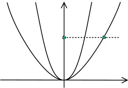
Figure 1: Marginal stability curve (MS) and Eckhaus instability curve (E) defining regions where plane waves solutions exist in the CGLe (inside (MS)), and are stable when $1+\alpha\beta>0$ (inside (E)). Case I corresponds to the wave of maximal possible wavenumber and Case II to the wave with $q=0$ and the maximal amplitude.

1.3 Coherent structures and MAWs

Coherent structures play a very important role in the study of pattern formation and dynamical properties of the CGLe [9]. They are uniformly propagating structures of the form

$$A(x,t)=R(x-vt)\exp({i\phi(x-vt)}e^{-i\omega t})$$

which can be expressed as solutions of a 3-$D$ nonlinear dynamical system obtained by substituting the above ansatz into the CGLe. There are two free parameters: the frequency $\omega$ and the group velocity $v$.

The fixed points of the 3-$D$ system are the plane waves described in the previous section. The homoclinic [11] and heteroclinic [9] connections between the fixed points correspond to localized coherent structures. The Nozaki-Bekki solutions [7] belong to this category; they connect asymptotic plane waves with different wavenumbers. In numerical simulations in large domains, nearly coherent structures are frequently observed in chaotic regimes, thus suggesting those objects are also relevant to spatiotemporally chaotic dynamics.

Recent numerical studies reveal another kind of coherent structure: modulated amplitude waves (MAWs) for the CGLe [12]. They correspond to limit cycles of the 3-$D$ nonlinear system. When $v=0$, MAWs are stationary. The formation of MAWs is the first instability encountered when a plane wave state crosses the Eckhaus or Benjamin-Feir stability line. The MAW structure is frequently observed in experiments [6, 20] and considered as a key to interpretation of patterns and bifurcations exhibited during the system’s transition to spatio-temporal chaos [13]. Traveling MAWs have been observed in numerical simulations of the CGLe in periodic boxes, with parameter $q$ between 0 and $\mu^{1/2}$, i.e., in between cases I and II; we are interested here only in stationary MAWs that appear either in case I or case II.

In this paper, we propose a new real-valued ODE to describe steady solutions of the CGLe. A 4-$D$ dynamical system derived from this ODE enables us to apply the successive approximation method [8], to prove the existence of stationary MAWs and to give the analytical form of the approximate solutions in both case I and case II. Numerical integrations of the exact CGLe are then compared to the approximate analytic result. Furthermore, we show non-analyticity at discrete points of solutions in case I, and prove the stability of the MAWs in case II. Some theorems needed in our proof are reproduced in the appendix B. In what follows, $\mathrm{diag}(\cdots)$ denotes a (block) diagonal matrix and $\mathrm{col}(\cdots)$ a column vector.

2 Stationary case

Since we are only interested in the steady solutions of the CGLe, we substitute the ansatz

$$A(x,t)=R(x)\exp({i\phi(x)-i\omega t}),\qquad(R,\phi)\in\mathbb{R}^{2}$$ (4)

into (1). We then have

$$(1+\alpha^{2})G_{x} =K \equiv(\beta-\alpha)R^{4}-(\omega-\mu\alpha)R^{2}$$ (5)

$$(1+\alpha^{2})G^{2} =M \equiv(1+\alpha^{2})R^{3}R_{xx}+(\alpha\omega+\mu)R^{4}-(1+\alpha\beta)R^{6}\,.$$ (6)

where $G\equiv\phi_{x}R^{2}$ is reminiscent of “angular momentum”. Note that if $\alpha=\beta$, this “angular momentum” is conserved — it is constant in space — provided that $\omega=\mu\alpha$. In that case, (6) can be solved in terms of elliptic functions [17]. We will only consider the case $\alpha\neq\beta$ in the following. Equations (5) and (6) are invariant under $(G,x)\rightarrow(-G,-x)$. Note that for plane waves, $K=0$ and $G$ is a constant. If $K$ is not always zero, differentiating (6) and dividing the result by (5) gives

$$2G=M_{x}/K\,,$$ (7)

and by (6)

$$M=\frac{1+\alpha^{2}}{4}\frac{M_{x}^{2}}{K^{2}}\,.$$ (8)

Furthermore, we can factorize $R^{2}$ from $M_{x}$ and $K$ and write $M_{x}=R^{2}N$ and $K=R^{2}P$, where

$$N \equiv (1+\alpha^{2})\frac{1}{2}(R^{2})_{xxx}+(\alpha\omega+\mu)2(R^{2})_{x}-(1+\alpha\beta)3R^{2}(R^{2})_{x}$$

$$P \equiv (\beta-\alpha)R^{2}-(\omega-\mu\alpha)\,.$$ (9)

The last relation can be used to express $R^{2}$ in terms of $P$:

$$R^{2}=\frac{(\omega-\mu\alpha)+P}{\beta-\alpha}=e+dP=R_{0}^{2}+\frac{P}{\beta-\alpha}\,,$$ (10)

where $d\equiv 1/(\beta-\alpha)$ and $e\equiv{(\omega-\mu\alpha)}/{(\beta-\alpha)}$.

Note that $e=R_{0}^{2}$ is the square of the homogeneous amplitude $R_{0}(q,\omega)$ of the Stokes plane wave solution (2) of frequency $\omega$ and wavevector $q(\omega)$. $P$ then appears as the modulation of the amplitude squared with respect to the Stokes solution, and so it is an appropriate variable to describe a MAW.

Substituting $K$ and $M_{x}$ into (8), we have

$$\frac{1+\alpha^{2}}{4}\frac{N^{2}}{P^{2}}=M\,.$$ (11)

If $P\neq 0$ (11) is equivalent to (5) and (6). It is easy to check that if we regard (7) as a definition of $G$, and use $K,M,N,P$ expressed in terms of $R$, equation (5) and (6) will be recovered as a result of (8) and (11). Differentiating both sides of (11) results in

$$\frac{1+\alpha^{2}}{2}(PN_{x}-NP_{x})=R^{2}P^{3}\,.$$ (12)

In this step we have extended the solution set of (11), because as we integrate (12) back, we get

$$\frac{1+\alpha^{2}}{4}\frac{N^{2}}{P^{2}}=M+{\mathcal{C}}\,,$$ (13)

where ${\mathcal{C}}$ is an integration constant. Only when ${\mathcal{C}}=0$, a solution of (12) is a solution of (11). For this reason, when obtaining solutions of (12), we have to check the consistency condition

$$\frac{1+\alpha^{2}}{4}\frac{N^{2}}{P^{2}}-M=0$$ (14)

to make sure that we have a solution of (11), thus a solution of (5) and (6). Note that if $K$ vanishes we have to go back to (5) and (6), since in that case (11) is not well defined. Let us rewrite $N$ in terms of $P$:

$$N=\displaystyle\frac{2}{1+\alpha^{2}}\left(aP_{xxx}+bP_{x}+cPP_{x}\right)\,,$$ (15)

where $a,b,c$ are constants

$$a \equiv \frac{(1+\alpha^{2})^{2}}{4(\beta-\alpha)}$$

$$b \equiv \frac{1+\alpha^{2}}{2}\left(\frac{2(\alpha\omega+\mu)}{\beta-\alpha}-\frac{3(1+\alpha\beta)(\omega-\mu\alpha)}{(\beta-\alpha)^{2}}\right)$$ (16)

$$c \equiv -\frac{3(1+\alpha\beta)(1+\alpha^{2})}{2(\beta-\alpha)^{2}}\,.$$

After some algebra (here relegated to appendix A), we get an equation for $P$ only:

$$\left(\frac{\tilde{M}_{x}}{P}\right)_{x}=\frac{\lambda}{a}\tilde{M}+kP\,,\qquad\tilde{M}\equiv\lambda P_{xx}+dP^{2}+\tilde{e}P\,.$$ (17)

$\lambda$ is a fixed real constant that depends on $\alpha$ and $\beta$ only, and that takes two different values given in appendix A. $\lambda$ is a transient variable used in the proof and derivation but our solutions to the CGLe do not depend on $\lambda$ and do not distinguish the two values of $\lambda$ (see section 4). $\tilde{e}$ and $k$ are real parameters introduced as $\tilde{e}+\frac{a}{\lambda}k=e$. So (17) has two free parameters: $\omega$, introduced by the ansatz (4) as the carrier frequency of the solution, and $k$. the consistency condition (14) fixes one parameter.

3 4-$D$ dynamical system and the existence of periodic solutions

Let us take $\tau$ as the spatial variable, $P=P(\tau)$ in (9), and rewrite (17) as a system of first order equations in $\tau$. With $\tilde{N}={\tilde{M}_{\tau}}/{P}$ and $Q=P_{\tau}$, from (17) we have

$$\left\{\begin{array}[]{rcl}\dot{\tilde{M}}&=&\tilde{N}P\\ \dot{\tilde{N}}&=&\frac{\lambda}{a}\tilde{M}+kP\\ \dot{P}&=&Q\\ \dot{Q}&=&\frac{1}{\lambda}(\tilde{M}-dP^{2}-\tilde{e}P)\end{array}\right.\,,$$ (18)

where the dot represents the derivation with respect to the spatial variable $\tau$.

It is easy to check that $P=0$ is a solution of the original equations (5) and (6), corresponding to the plane wave solution of the CGLe with frequency $\omega$. We will study the behavior near $P=0$ and prove the existence of periodic solutions for small $P$. In the CGLe, this corresponds to a weakly modulated amplitude wave which bifurcates from a plane wave solution. If $P\sim\epsilon$, where $\epsilon$ is a small parameter, so are $\tilde{M},\tilde{N},Q$ by their definitions. Write

$$(\tilde{M},\tilde{N},P,Q)=(\epsilon x,\epsilon y,\epsilon z,\epsilon w)$$

and set $k=k_{1}+\epsilon k_{2}$. Substituting these into the 4-$D$ system, we have

$$\frac{d}{d\tau}\left(\begin{array}[]{c}x\\ y\\ z\\ w\end{array}\right)=A\left(\begin{array}[]{c}x\\ y\\ z\\ w\end{array}\right)+\epsilon\left(\begin{array}[]{c}y\,z\\ k_{2}\,z\\ 0\\ -\frac{d}{\lambda}z^{2}\end{array}\right),\mbox{ where }A=\left(\begin{array}[]{cccc}0&0&0&0\\ \frac{\lambda}{a}&0&k_{1}&0\\ 0&0&0&1\\ \frac{1}{\lambda}&0&\frac{-\tilde{e}}{\lambda}&0\end{array}\right).$$

The linear part $A$ describes the behavior of the system in the neighborhood of the trivial fixed point $(0,0,0,0)$. Note that the system is invariant under $(t,y,w)\rightarrow-(t,y,w)$. We use this property to simplify our analysis. Moreover, this system defines an incompressible flow since $\nabla\cdot\vec{X}=0$, where $\vec{X}=(x,y,z,w)$. It follows from (13) that the system has one integration constant ${\mathcal{C}}$. This constant induces a foliation of the phase space into three-dimensional manifolds. Physical solutions, i.e., the solutions of the original CGLe, are restricted to ${\mathcal{C}}=0$, the manifold that satisfies the consistency condition (14).

These properties strongly restrict the possible distribution of eigenvalues of $A$. We restrict our analysis to the case ${\tilde{e}}/{\lambda}>0$, then $A$ has eigenvalues $\left\{0,0,i\omega_{1},-i\omega_{1}\right\}$ with $\omega_{1}=\sqrt{{\tilde{e}}/{\lambda}}$. In that case, periodic solutions or MAWs can exist as we will prove in the following. The evolution of the system along either of the two degenerate eigenvalue 0 directions respects the constant ${\mathcal{C}}$ foliation: if the solution is on a constant ${\mathcal{C}}$ manifold at initial time, it remains there for any later time.

We now discuss the condition $\tilde{e}/\lambda>0$ in terms of an instability of the underlying plane wave. We can rewrite $\tilde{e}/\lambda$ using (16) and (52). Assuming that the solution we are searching for is close to a plane wave, we can use the wavenumber $q$ instead of the frequency $\omega$, using the dispersion relation (2) for plane waves:

$$\frac{\tilde{e}}{\lambda}=\frac{b}{a} = \frac{2}{1+\alpha^{2}}\left[2(\alpha\omega+\mu)-\frac{3(1+\alpha\beta)(\omega-\mu\alpha)}{\beta-\alpha}\right]$$

$$= \frac{2}{1+\alpha^{2}}\left[(3+\alpha\beta+2\alpha^{2})q^{2}-(1+\alpha\beta)\mu\right]\,.$$

If we write

$$q_{\rm M}^{2}\equiv\frac{(1+\alpha\beta)\mu}{3+\alpha\beta+2\alpha^{2}}\,,$$ (20)

we have

$$\frac{\tilde{e}}{\lambda}>0 \Leftrightarrow \left|\begin{array}[]{rl}q^{2}>q_{\rm M}^{2}&\quad{\rm if}\quad(1+\alpha\beta)>0\\ q^{2}<q_{\rm M}^{2}&\quad{\rm if}\quad(1+\alpha\beta)<-2(1+\alpha^{2})\\ \forall q\in[-\sqrt{\mu},\sqrt{\mu}]&\quad{\rm if}\quad-2(1+\alpha^{2})<1+\alpha\beta<0\end{array}\right..$$ (24)

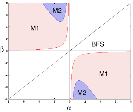
Figure 2: Left: wavenumber distribution of stationary MAWs in the $(\alpha,\beta)$ plane. In (BFS), MAWs exist if $q^{2}>q_{\rm M}^{2}$. In (M1), MAWs exist $\forall q$. In (M2), MAWs exist if $q^{2}<q_{\rm M}^{2}$. Right: regions of existence of MAWs in the $(q,\mu)$ plane in the Benjamin-Feir-Newell stable regime ((BFS) region). (MS) is the marginal stability curve, (E) is the Eckhaus instability curve and (M) is existence curve defined by (20). Stationary MAWs exist outside (M).

The corresponding regions are illustrated on Fig. 2. Note that $q_{\rm M}(\alpha,\beta,\mu)=q_{\rm E}(\beta,\alpha,\mu)$. If $|\alpha|=|\beta|$, the positivity of $\tilde{e}/\lambda$ is assured when the corresponding plane wave is Eckhaus unstable. If $|\alpha|\neq|\beta|$, the positivity does not coincide anymore with the Eckhaus criterion; this is not surprising considering that we do not restrict our analysis to long wavelength perturbations of plane waves, but that the solutions we are seeking may have any wavenumber.

In the following we distinguish two cases. In the first case eigenvalue $0$ has a simple elementary divisor, i.e., has two distinct eigenvectors citejhale. This coincides with case I: the MAW solution bifurcates from the $A=0$ state, with $\omega\sim\mu\alpha$ and hence ${\tilde{e}}/{\lambda}\sim 4\mu>0$, for $\mu>0$. In the second case, eigenvalue $0$ has only one eigenvector. This coincides with case II: the MAW is superimposed over a plane wave with $\omega\simeq\mu\beta$, so $q\simeq 0$, and

$$\frac{\tilde{e}}{\lambda}\simeq-\frac{2\mu(1+\alpha\beta)}{1+\alpha^{2}}>\,0,$$

The positivity is insured if the system is Benjamin-Feir-Newell unstable, $(1+\alpha\beta)<0$.

In terms of $\tilde{M},\tilde{N},P,Q$, the consistency condition (14) can be written as

$$(1+\alpha^{2})M=\left(\frac{a}{\lambda}\tilde{N}-\lambda Q\right)^{2}$$ (25)

where in new variables

$$M = \frac{d(1+\alpha^{2})}{2\lambda}(d\,P+e)(\tilde{M}-d\,P^{2}-\tilde{e}\,P)-\frac{d^{2}(1+\alpha^{2})}{4}\,Q^{2}$$

$$(\alpha\omega+\mu)(d\,P+e)^{2}-(1+\alpha\,\beta)(d\,P+e)^{3}\,.$$

Recalling (6), we may express $G$ by

$$G=\frac{\frac{a}{\lambda}\tilde{N}-\lambda Q}{1+\alpha^{2}}\,.$$ (26)

Here we are allowed to fix the sign of the right hand side expression because of the $(G,x)\mapsto(-G,-x)$ reflection symmetry of (5) and (6).

3.1 Case I

We want the eigenvalue $0$ to have non-degenerate eigenvectors, for this, we set

$$\frac{\frac{\lambda}{a}}{\frac{1}{\lambda}}=\frac{k_{1}}{-\frac{\tilde{e}}{\lambda}},\mbox{~{}i.e.,~{}}k_{1}=-\frac{\lambda\tilde{e}}{a}$$

Consequently, we have

$$e=\tilde{e}+\frac{a}{\lambda}k=\frac{\epsilon a}{\lambda}k_{2}\,.$$ (27)

Notice that $e\sim 0$ to the zeroth order, so $R_{0}\sim 0$ and $\omega\sim\mu\alpha$, which means that the solution to be considered bifurcates from the zero solution $A=0$, corresponding to a plane wave around the marginal stability curve, with wavenumber $q\sim\pm\mu^{1/2}$. This solution is therefore outside the Eckhaus stability region when $1+\alpha\beta>0$.

The four eigenvectors of $A$ are:

$$\left(\begin{array}[]{c}0\\ 1\\ 0\\ 0\end{array}\right)\qquad\left(\begin{array}[]{c}\tilde{e}\\ 0\\ 1\\ 0\end{array}\right)\qquad\left(\begin{array}[]{c}0\\ -ik_{1}\omega_{1}^{-1}\\ 1\\ i\omega_{1}\end{array}\right)\qquad\left(\begin{array}[]{c}0\\ ik_{1}\omega_{1}^{-1}\\ 1\\ -i\omega_{1}\end{array}\right)\,.$$

Let

$$D=\left(\begin{array}[]{rccl}0&\tilde{e}&0&0\\ 1&0&0&\frac{\lambda^{2}}{a}\\ 0&1&1&0\\ 0&0&0&1\end{array}\right),D^{-1}=\left(\begin{array}[]{rccl}0&1&0&-a^{-1}{\lambda^{2}}\\ {\tilde{e}^{-1}}&0&0&0\\ -{\tilde{e}^{-1}}&0&1&0\\ 0&0&0&1\end{array}\right).$$

and $\vec{\tilde{X}}\equiv(\tilde{x},\tilde{y},\tilde{z},\tilde{w})=D^{-1}\vec{X}$. The dynamical equations for the new variables become

$$\frac{d}{d\tau}\vec{\tilde{X}}=M(\omega_{1})\vec{\tilde{X}}+\epsilon\left(\begin{array}[]{c}k_{2}(\tilde{y}+\tilde{z})+\frac{\lambda d}{a}(\tilde{y}+\tilde{z})^{2}\\ \frac{1}{\tilde{e}}(\tilde{x}+\frac{\lambda^{2}}{a}\tilde{w})(\tilde{y}+\tilde{z})\\ -\frac{1}{\tilde{e}}(\tilde{x}+\frac{\lambda^{2}}{a}\tilde{w})(\tilde{y}+\tilde{z})\\ -\frac{d}{\lambda}(\tilde{y}+\tilde{z})^{2}\end{array}\right)\,,$$

where

$$M(\omega_{1})=D^{-1}AD=\left(\begin{array}[]{rccl}0&0&0&0\\ 0&0&0&0\\ 0&0&0&1\\ 0&0&-\omega_{1}^{2}&0\end{array}\right)\,.$$

The angular frequency of the solution $\Omega$ should be close to $\omega_{1}$, $\Omega^{2}=\omega_{1}^{2}+\epsilon\gamma$, with the shift $\gamma$ to be determined later. Next, we change variables to:

$$\left\{\begin{array}[]{rcl}\tilde{x}&=&x_{1}\\ \tilde{y}&=&x_{2}\\ \tilde{z}&=&z_{1}\,\sin\Omega\tau+z_{2}\,\cos\Omega\tau\\ \tilde{w}&=&\Omega z_{1}\,\cos\Omega\tau-\Omega z_{2}\,\sin\Omega\tau\end{array}\right.$$ (28)

The 4-$D$ system of equations then takes form:

$$\dot{x_{1}} = \epsilon\,\left[k_{2}(x_{2}+z_{1}\sin\Omega\tau+z_{2}\cos\Omega\tau)+\frac{\lambda d}{a}(x_{2}+z_{1}\sin\Omega\tau+z_{2}\cos\Omega\tau)^{2}\right]$$

$$\dot{x_{2}} = \frac{\epsilon}{\tilde{e}}\left[x_{1}+\frac{\Omega\lambda^{2}}{a}(z_{1}\cos\Omega\tau-z_{2}\sin\Omega\tau)\right](x_{2}+z_{1}\sin\Omega\tau+z_{2}\cos\Omega\tau)$$

$$\dot{z_{1}} = \frac{\epsilon}{\Omega}\left[-\frac{d}{\lambda}(x_{2}+z_{1}\sin\Omega\tau+z_{2}\cos\Omega\tau)^{2}\cos\Omega\tau\right.$$

$$\quad+\gamma(z_{1}\sin\Omega\tau+z_{2}\cos\Omega\tau)\cos\Omega\tau$$

$$\quad\left.-\frac{\Omega}{\tilde{e}}\left(x_{1}+\frac{\Omega\lambda^{2}}{a}(z_{1}\cos\Omega\tau-z_{2}\sin\Omega\tau)\right)(x_{2}+z_{1}\sin\Omega\tau+z_{2}\cos\Omega\tau)\sin\Omega\tau\right]$$

$$\dot{z_{2}} = \frac{\epsilon}{\Omega}\left[\frac{d}{\lambda}(x_{2}+z_{1}\sin\Omega\tau+z_{2}\cos\Omega\tau)^{2}\sin\Omega\tau\right.$$

$$\quad-\gamma(z_{1}\sin\Omega\tau+z_{2}\cos\Omega\tau)\sin\Omega\tau$$

$$\quad\left.-\frac{\Omega}{\tilde{e}}\left(x_{1}+\frac{\Omega\lambda^{2}}{a}(z_{1}\cos\Omega\tau-z_{2}\sin\Omega\tau)\right)(x_{2}+z_{1}\sin\Omega\tau+z_{2}\cos\Omega\tau)\cos\Omega\tau\right]$$

The proof of the existence of weak MAWs close to $P=0$ relies on a series of theorems from J. Hale’s monograph [8]. We reproduce the relevant theorems in appendix B, and refer to them as the need arises.

Note that the transformation $(\tau,x_{1},x_{2},z_{1},z_{2})\rightarrow(-\tau,-x_{1},x_{2},-z_{1},z_{2})$ leaves the system (3.1) invariant. So, by definition B.1 of appendix B the system has the property $E$ with respect to $Q$, with

$$Q=\mathrm{diag}(-1,1,-1,1)\,.$$

As we are interested only in the solutions with definite parity, we may start the iteration with the vector

$$\vec{X_{0}}=(0,a_{2},0,a_{4})\,.$$

According to Theorem B.4, our solution $z(\tau,\vec{X_{0}},\epsilon)$ has the property

$$Qz(-\tau,\vec{X_{0}},\epsilon)=z(\tau,\vec{X_{0}},\epsilon)\,,$$

which means that our solutions are either symmetric or antisymmetric. According to Theorem B.5, the second and the fourth determining equations are always zero for this starting vector. For the first and the third determining equations, the zeroth order solution of $\vec{\tilde{X}}$ , i.e. $\vec{X_{0}}$, may be substituted, and we get

$$k_{2}a_{2}+\frac{\lambda d}{a}(a_{2}^{2}+\frac{1}{2}a_{4}^{2}) = 0$$ (30)

$$\frac{\gamma}{2\Omega}a_{4}+\frac{\lambda^{2}\Omega a_{2}a_{4}}{2a\tilde{e}}-\frac{d}{\lambda\Omega}\,a_{2}a_{4} = 0\,.$$ (31)

From (31), we have two possibilities: either $a_{4}=0$ or

$$\gamma+a_{2}\left(\frac{\lambda^{2}\Omega^{2}}{a\tilde{e}}-\frac{2d}{\lambda}\right)=0\,.$$ (32)

When $a_{4}=0$, using $\vec{X_{0}}=(0,a_{2},0,0)$ in (3.1) leads to a trivial constant solution. In the following, we consider only the second case (32). We can solve (30) and (32) for $\gamma$ and $a_{4}$ and prove that the system (3.1) has periodic solutions. Note that we have three free parameters $\epsilon,a_{2},k_{2}$. But as we will see further, $\epsilon$ and $a_{2}$ are always combined as $\epsilon a_{2}$ in the first approximation controlling the amplitude and the period of the solution, and the combination will therefore be regarded here as one single free parameter. For general periodic solutions, $a_{2}$ can be interpreted as a phase control parameter, i.e., a parameter giving the initial location on the periodic orbit at $\tau=\tau_{0}$. Here, because we only consider symmetric solutions, the translational symmetry of the autonomous system is broken, and that is the reason why $\epsilon$ and $a_{2}$ combine into a single parameter. The remaining parameter $k_{2}$ can be chosen freely, for example as to satisfy the consistency condition (25), which, when the zeroth order solution is substituted, becomes at order $(\epsilon^{2})$:

$$-\frac{d^{2}}{4}\,\Omega^{2}\,a_{4}^{2}+\mu\left(da_{2}+\frac{k_{2}a}{\lambda}\right)^{2}=0\,.$$ (33)

At zeroth order, $\Omega^{2}=\omega_{1}^{2}=4\mu$ and $\tilde{e}=4\mu\lambda$. Solving the system of equations (30),(32) and (33), we get

$$\left\{\begin{array}[]{rcl}k_{2}&=-&\frac{3\lambda}{a}da_{2}\\ \gamma&=&\frac{c}{a}a_{2}\\ a_{4}&=&\pm 2a_{2}\end{array}\right.\,.$$

We can write out the Jacobian for those three equations explicitly:

$$J=\left(\begin{array}[]{ccc}a_{2}&0&\frac{\lambda d}{a}a_{4}\\ 0&1&0\\ \frac{2\mu a}{\lambda}(da_{2}+\frac{k_{2}a}{\lambda})&0&-\frac{d^{2}}{2}\Omega^{2}a_{4}\end{array}\right)\,.$$

The determinant of this Jacobian is

$$\det J=\frac{1}{2}d^{2}\Omega^{2}a_{2}a_{4}\neq 0\qquad a_{2}\neq 0\,.$$

We now invoke theorem B.2, reproduced in appendix B, and conclude our proof that system (5) and (6) has periodic solutions near $P=0$. We shall give approximate solutions in section 4, and show that in this case they contain defects.

3.2 Case II

Eigenvalue 0 has only one eigenvector. In this case, we assume that $\frac{\lambda}{a}\tilde{e}+k_{1}\neq 0$ to the zeroth order in $\epsilon$, so without loss of generality we can choose $k_{2}=0$. Then $\frac{\lambda}{a}e=\frac{\lambda}{a}\tilde{e}+k_{1}$. Implementing the transformation $\vec{X}=D\vec{\tilde{X}}$ with

$$D=\left(\begin{array}[]{cccc}0&\tilde{e}&0&0\\ 1&0&0&-k_{1}\omega_{1}^{-2}\\ 0&1&1&0\\ 0&0&0&1\end{array}\right)$$

we have

$$\frac{d}{d\tau}\vec{\tilde{X}}=M(\omega_{1})\vec{\tilde{X}}+\epsilon\left(\begin{array}[]{c}-\frac{d}{\tilde{e}}k_{1}(\tilde{y}+\tilde{z})^{2}\\ \frac{1}{\tilde{e}}(\tilde{x}-k_{1}\frac{\lambda}{\tilde{e}}\tilde{w})(\tilde{y}+\tilde{z})\\ -\frac{1}{\tilde{e}}(\tilde{x}-k_{1}\frac{\lambda}{\tilde{e}}\tilde{w})(\tilde{y}+\tilde{z})\\ -\frac{d}{\lambda}(\tilde{y}+\tilde{z})^{2}\end{array}\right)\,,$$

where

$$M(\omega_{1})=D^{-1}AD=\left(\begin{array}[]{rccl}0&\frac{\lambda e}{a}&0&0\\ 0&0&0&0\\ 0&0&0&1\\ 0&0&-\omega_{1}^{2}&0\end{array}\right)\,.$$

As in case I, let $\Omega^{2}=\omega_{1}^{2}+\epsilon\gamma$ and perform the same transformation (28) into variables $x_{1},x_{2},z_{1},z_{2}$. We then obtain a 4-$D$ system similar to (3.1). However, in the equation for $\dot{x_{1}}$, there is an $\epsilon$-free term. In order to use the successive approximation method, further transformations are required. Let $\rho\in\mathbb{R}$ such that $\rho^{2}=\epsilon$. With the transformation $x_{2}\rightarrow\rho x_{2},\epsilon\rightarrow\rho^{2}$ we recover the standard form

$$\dot{x_{1}} = \frac{\rho\lambda e}{a}x_{2}-\rho^{2}k_{1}\frac{d}{\tilde{e}}(\rho x_{2}+z_{1}\,\sin\Omega\tau+z_{2}\,\cos\Omega\tau)^{2}$$

$$\dot{x_{2}} = \frac{\rho}{\tilde{e}}\left[x_{1}-k_{1}\frac{\Omega\lambda}{\tilde{e}}(z_{1}\,\cos\Omega\tau-z_{2}\sin\Omega\tau)\right](\rho x_{2}+z_{1}\sin\Omega\tau+z_{2}\cos\Omega\tau)$$

$$\dot{z_{1}} = \frac{\rho^{2}}{\Omega}\left[\frac{-d}{\lambda}(\rho x_{2}+z_{1}\sin\Omega\tau+z_{2}\cos\Omega\tau)^{2}\cos\Omega\tau\right.$$

$$+\gamma(z_{1}\sin\Omega\tau+z_{2}\cos\Omega\tau)\cos\Omega\tau$$

$$-\frac{\Omega}{\tilde{e}}\left.\left(x_{1}-\frac{\Omega\lambda}{\tilde{e}}k_{1}\,(z_{1}\,\cos\Omega\tau-z_{2}\sin\Omega\tau)\right)(\rho x_{2}+z_{1}\sin\Omega\tau+z_{2}\cos\Omega\tau)\sin\Omega\tau\right]$$

$$\dot{z_{2}} = \frac{\rho^{2}}{\Omega}\left[\frac{d}{\lambda}(\rho x_{2}+z_{1}\sin\Omega\tau+z_{2}\cos\Omega\tau)^{2}\sin\Omega\tau\right.$$

$$-\gamma(z_{1}\sin\Omega\tau+z_{2}\cos\Omega\tau)\sin\Omega\tau$$

$$-\frac{\Omega}{\tilde{e}}\left.\left(x_{1}-\frac{\Omega\lambda}{\tilde{e}}k_{1}(z_{1}\,\cos\Omega\tau-z_{2}\sin\Omega\tau)\right)(\rho x_{2}+z_{1}\sin\Omega\tau+z_{2}\cos\Omega\tau)\cos\Omega\tau\right]\,,$$

The system (3.2) has the same symmetry as identified in the case I. If we are only interested in solutions with definite parity, we may again start the iteration with $\vec{X_{0}}=(0,a_{2},0,a_{4})$. To the second order $(\rho^{2})$, the determining equations are:

$$a_{2}\frac{\lambda e}{a}-\rho\frac{da_{4}^{2}k_{1}}{2\tilde{e}}+0(\rho^{3}) = 0$$ (37)

$$\rho\frac{\gamma a_{4}}{2\Omega}-\rho^{2}\left(\frac{da_{2}a_{4}}{\lambda\Omega}+\frac{\lambda\Omega a_{2}a_{4}k_{1}}{2\tilde{e}^{2}}\right)+0(\rho^{3}) = 0\,.$$ (38)

From the second equation we obtain either $a_{4}=0$ (trivial for our purposes, as discussed above) or

$$\gamma-\rho a_{2}\left(\frac{2d}{\lambda}+\frac{\lambda\Omega^{2}k_{1}}{\tilde{e}^{2}}\right)+0(\rho^{2})=0\,.$$ (39)

If we backtrack the transformations made, it is clear that the consistency condition requires that we keep terms up to the fourth order $(\rho^{4})$. We found that with the substitution

$$e=\frac{\alpha\omega+\mu}{1+\alpha\beta}+\rho^{2}(\rho^{2}\omega_{3}-\rho da_{2})\,,$$

where $\omega_{3}$ is a new parameter, only the fourth or higher order terms are left in the consistency condition. From the definition $e=R_{0}^{2}=(\omega-\mu\alpha)/(\beta-\alpha)$ and the above equation, we get $\omega\sim\mu\beta$ and then $e\sim\mu$ to the zeroth order. So $R_{0}\sim\sqrt{\mu}$, $q\sim 0$, which means that this solution bifurcates from the HOS $A=\sqrt{\mu}\exp({-i\omega t})$. To the leading order ($\rho^{4}$), we are allowed to use the following substitutions in the consistency condition (25):

$$a_{2}\rightarrow 0\quad\omega\rightarrow\mu\beta\quad\Omega\rightarrow\sqrt{-\frac{2\mu(1+\alpha\beta)}{1+\alpha^{2}}},$$

$$k_{1}\rightarrow\frac{\mu\lambda}{a}\left(1+\frac{2\lambda(1+\alpha\beta)}{1+\alpha^{2}}\right)\quad\tilde{e}\rightarrow-\frac{2\mu\lambda(1+\alpha\beta)}{1+\alpha^{2}}\,.$$ (40)

The resulting equation is of a relatively simple form:

$$a_{4}^{2}(-\lambda+d^{2}(1+\alpha\beta)(1+\alpha^{2}+\lambda+\lambda\alpha\beta))+4(1+\alpha\beta)^{2}\lambda\mu\omega_{3}=0\,.$$ (41)

From (37) it follows that $a_{2}$ is of order $\rho$, and from (39) that $\gamma\sim 0(\rho^{2})$. After a change of variable $a_{2}=\rho\,a_{22}$ and keeping only the highest order for the equations, we can rewrite (37) and (39) as

$$a_{22}\frac{\lambda e}{a}-\frac{k_{1}da_{4}^{2}}{2\tilde{e}} = 0$$ (42)

$$\gamma = 0.$$ (43)

For $e,\tilde{e},k_{1}$ we use the values in (40). From (42), (43) and (41), we can solve for $a_{22},\gamma,\omega_{3}$. The Jacobian of those equations is

$$J=\left(\begin{array}[]{ccc}\frac{\lambda e}{a}&0&0\\ 0&1&0\\ 0&0&4(1+\alpha\beta)^{2}\lambda\mu\end{array}\right),$$

So, $\det J=4(1+\alpha\beta)^{2}\lambda^{2}\mu e/a\neq 0$ for $1+\alpha\beta\neq 0$. According to Theorem B.2, we have proved that equations (5) and (6) possess periodic solutions.

4 Analytic form of periodic solutions, stability analysis and numerical tests

We have proved in the preceding section the existence of symmetric periodic solutions in case I and II. In both cases, a small parameter $\epsilon$ or $\rho$ ensures the convergence of successive approximations. However, we did not give a bound on the highest value of this parameter, nor did we show that the solutions which we obtain are the ones observed in numerical simulations. In this section we give the approximate analytical form of periodic solutions. We compare them with direct numerical integration of the CGLe in case II.

The solutions are shown to be independent of $\lambda$ to order $\epsilon$ in case I and to order $\epsilon^{2}$ in case II. In addition, these solutions should also satisfy the 3-$D$ ODE mentioned in section 1.3 which do not contain $\lambda$, so they can be matched with the solutions of the 3-$D$ system in a unique way, independent of the value of $\lambda$. Hence, we conclude that to all orders the physical solutions are identical for the two values of $\lambda$.

The two cases are taken separately. In this section, we reinstate $x$ as the spatial variable, $R=R(x)$.

4.1 Case I

Using (10), (26) and the case I calculations of the preceding section, we have after some algebra:

$$R^{2} = -2\epsilon da_{2}(1\pm\cos\Omega x)$$ (44)

$$\phi_{x} = -\frac{\epsilon a_{2}}{2(1+\alpha^{2})\Omega}\frac{\sin 2\Omega x\pm 2\sin\Omega x}{1\pm\cos\Omega x}\,.$$

To the first order of $\epsilon$, $R$ and $\phi_{x}$ are independent of $\lambda$. The $\pm$ sign selects two solutions which transform into each other by translating by a half period. This is reminiscent of the spatial translational invariance in the symmetric solution space. From the definitions of $e,\Omega$ and from (27), (3), we get to the first order:

$$\omega = \mu\alpha-3\epsilon a_{2}$$

$$\omega_{1}^{2} = 4\mu+\frac{6\epsilon da_{2}}{1+\alpha^{2}}(\alpha\beta+2\alpha^{2}+3)$$

$$\Omega = \omega_{1}+\frac{\epsilon\gamma}{2\omega_{1}}\,.$$ (45)

We see that $\omega$ and $\Omega$ are independent of $\lambda$. On the other hand, for periodic boundary conditions, we can use Fourier modes directly to transform the PDE (1) to a finite set of approximate ODE’s by Galerkin truncation. Then the stationary solution can be obtained by solving a set of nonlinear algebraic equations.

Numerical comparison

If we take as an example the following parameter values (previously used in [21]) for which defect chaos is expected:

$$\alpha=1.5,\quad\beta=-1.2$$

and fix the size of the domain to $L=24$, then at $\mu=0.072644$, $\omega=0.097879$, a periodic solution of period $L/2$ is found. This solution has $R_{max}\simeq 0.0750$. On the other hand, if we use the same $\alpha,\beta,\mu$ and search for $R_{max}\simeq 0.075$ by adjusting $\epsilon$ (we always keep $a_{2}=1$), we find that

$$\epsilon\sim 0.00380,\quad\omega=0.097566,\quad\mbox{ period }\frac{2\pi}{\Omega}=12.0102\,.$$

The approximate analytic solution and the numerical solution of the exact CGLe agree very well. The profile of $R$ from our successive approximation is shown in Fig. 3.

Figure 3: Spatial profile of the amplitude $R(x)$ at $\mu=0.072644$, from (44) with $R_{max}=0.075$.

Structure near the defect

It is easy to see from (44) that only $\epsilon a_{2}>0$ is the physically interesting combination. However, we may wonder whether it is really true that $R^{2}=dP+e$ remains non-negative everywhere while touching zero at some points. Fig. 3 and the first equation of (44) suggest a positive answer to this question. But since we have only an approximate solution, further justification is needed. Suppose at some instant $x_{0}$, we have $dP+e=0$ on the periodic orbit. From the consistency condition (25), at this transition point

$$\frac{d^{2}(1+\alpha^{2})}{4}Q^{2}+\left(\frac{a}{\lambda}\tilde{N}-\lambda Q\right)^{2}=0,$$

so, $Q=\tilde{N}=0$. According to (18), $\dot{\tilde{M}}=0$ and $\dot{P}=0$. Assume that $\dot{Q}=0$, then $\dot{\tilde{N}}\neq 0$ since the point is not an equilibrium. At next instant $x_{0}+\delta x$, the consistency condition can not be satisfied as the two sides of (25) have different orders of $\delta x$. So we conclude that $\dot{Q}\neq 0$ at the point $x_{0}$, which means that $Q(x_{0}+\delta x)$ has negative sign to that of $Q(x_{0}-\delta x)$. Thus, after touching the zero value plane, $dP+e$ returns to the positive half space again. The turning happens exactly on the $dP+e=0$ plane. We claim that $dP+e\geq 0$ always holds and the equality holds periodically. From (44), in the neighborhood of $R=0$ at $x=x_{0}$ on the periodic orbit, $R$ behaves like

$$R\sim\left(\frac{d\dot{Q}}{2}\right)^{1/2}|x-x_{0}|\,,$$

and is manifestly a non-analytic function of $x$.

We do not discuss the stability of the solutions in case I, as this has already been accomplished by Takáč [16] who has proven that these solutions are unstable.

4.2 Case II

To the first order of $\epsilon$, the solutions are

$$\left\{\begin{array}[]{rcl}x_{1}&=&-\frac{\epsilon k_{1}a_{4}^{2}}{8\tilde{e}^{2}\Omega}(2d\tilde{e}+\lambda k_{3})\sin 2\Omega x\\ x_{2}&=&\epsilon(a_{2}^{2}-\frac{\lambda k_{1}a_{4}^{2}}{4\tilde{e}^{2}}\cos 2\Omega x)\\ z_{1}&=&-\frac{\epsilon a_{4}^{2}}{12\tilde{e}^{2}\lambda\Omega^{2}}(3(3d\tilde{e}^{2}+\lambda^{2}\Omega^{2}k_{1})\sin\Omega x+(d\tilde{e}^{2}-\lambda^{2}\Omega^{2}k_{1})\sin 3\Omega x)\\ z_{2}&=&a_{4}+\frac{\epsilon a_{4}^{2}}{12\tilde{e}^{2}\lambda\Omega^{2}}(3(\lambda^{2}\Omega^{2}k_{1}-d\tilde{e}^{2})\cos\Omega x+(\lambda^{2}\Omega^{2}k_{1}-d\tilde{e}^{2})\cos 3\Omega x)\,,\\ \end{array}\right.$$

where $\epsilon=\rho^{2}>0$, and $a_{4}$ is a free parameter. In the following, we will see that $\epsilon$ and $a_{4}$ always emerge in the combination $\epsilon\,a_{4}$. To the second order, $\omega$ is

$$\omega=\mu\beta+\frac{\epsilon^{2}a_{4}^{2}}{4\mu(1+\alpha^{2})}\left(\frac{1+\alpha\,\beta}{\beta-\alpha}+\frac{\beta-\alpha}{1+\alpha\,\beta}\right)\,.$$

It is independent of $\lambda$, and therefore $e,b,\Omega$ are also independent of $\lambda$. $R$ and $\phi_{x}$ can also be calculated to the second order:

$$R^{2} = -\frac{d^{2}}{2\mu}(\epsilon a_{4})^{2}+d\epsilon a_{4}\cos\Omega x+\frac{d(\epsilon a_{4})^{2}}{12\Omega^{2}}\left(\frac{c}{a}+\frac{e}{b}\right)\cos 2\Omega x+e$$ (46)

$$\phi_{x} = \frac{\epsilon a_{4}}{\mu\Omega(1+\alpha^{2})}\left[e\sin\Omega x-\frac{\epsilon a_{4}}{24\Omega^{2}}\left(6d\Omega^{2}+\frac{7e^{2}}{a\Omega^{2}}+\frac{7ce}{a}\right)\sin 2\Omega x\right]$$

So clearly $R$ and $\phi_{x}$ are independent of $\lambda$. Similarly, the different signs of $a_{4}$ will give the same solution up to a half-period translation. This solution is the one observed in the numerics when passing the Eckhaus instability for underlying wavevector $q=0$. Linear stability analysis reveals [18] that the $q=0$ state, the most stable state under the long wavelength perturbations, becomes unstable when the size of the system is such that the smallest possible nonzero wavenumber $k$ satisfies

$$k^{2}<-\frac{2\mu(1+\alpha\beta)}{1+\alpha^{2}}\equiv\kappa^{2}\,.$$

It is easy to see that $\kappa^{2}=\omega_{1}^{2}$ up to order $(\rho^{4})$.

For our parameter choices $\mu=1,\alpha=1.5,\beta=-1.2$, the bifurcation size of the system is $L_{0}=\frac{2\pi}{\kappa}=8.95492$. In the following, we will first prove the stability of our solutions near the bifurcation point. Then we will compare them with the stable solutions observed in numerics.

Stability analysis: presentation

Assume that $A=R\exp({i\phi})$ where $R,\phi\in\mathbb{R}$ is an exact solution of (1). The perturbed solution is assumed to be $\bar{A}=(R+r)\exp({\phi+\theta})$, where $r,\theta\in\mathbb{R}$ is the perturbation on the amplitude and phase, separately. Substitute it into (1), keeping only the linear terms in $r$ and $\theta$. We have

$$r_{t} = (\mu-\phi_{x}^{2}-\alpha\phi_{xx}-3R^{2})r+r_{xx}-2\alpha\phi_{x}r_{x}$$ (47)

$$-(2R\phi_{x}+2\alpha R_{x})\theta_{x}-\alpha R\theta_{xx}$$

$$R\theta_{t} = (\omega-\alpha\phi_{x}^{2}+\phi_{xx}-3\beta R^{2})r+\alpha r_{xx}+2\phi_{x}r_{x}$$ (48)

$$+(2R_{x}-2\alpha R\phi_{x})\theta_{x}+R\theta_{xx}\,,$$

where in (48) we have used $\phi_{t}=-\omega$. To study the stability of the starting solution $A$, we treat these equations as an eigenvalue problem for a two components vector, i.e., we let $r_{t}=\sigma r$, $\theta_{t}=\sigma\theta$ and we investigate the spectra $\sigma$ of the linear operator resulting from (47) and (48) in the $C^{1}$ continuous periodic function space. As the CGLe has global phase invariance, the eigenvalue equations always have solution $(r,\theta)=(0,\theta_{0})$ with eigenvalue $\sigma=0$. At the same time, spatial translational invariance implies that another eigenmode has $\sigma=0$. As a result, saying that the solution is stable means that it is stable up to a phase and a spatial translation, and that all other eigenmodes have eigenvalues with negative real parts.

Invoking the expression for $R,\phi_{x}$ to the second order of $\epsilon$, the coefficients of various terms of $r,\theta$ and their derivatives in (47) and (48) become explicit functions of $x$. The resulting linear operator on $(r,\theta)$ has even parity due to the symmetry of our solution, and we can consider the even and odd solutions of $r,\theta$ separately. If we set $\epsilon=0$, i.e., the starting state $A$ is a plane wave state, then $\cos(n\Omega x)$ and $\sin(n\Omega x)$ are the eigenfunctions of the unperturbed linear operator. They give the stability spectrum of the plane waves. Now, let us move a little (to the order of $\epsilon$) beyond the bifurcation point. The eigenfunctions are still $\cos(n\Omega x)$ and $\sin(n\Omega x)$ up to $\epsilon$ corrections. For example, if the even solutions are considered first, we assume that to the first order the eigenfunctions are (the time dependence for $r,\theta$ has been suppressed):

$$r = m_{1}\cos(n\Omega x)+\epsilon(m_{0}\cos((n-1)\Omega x)+m_{2}\cos((n+1)\Omega x))$$ (49)

$$\theta = n_{1}\cos(n\Omega x)+\epsilon(n_{0}\cos((n-1)\Omega x))+n_{2}\cos((n+1)\Omega x))\,,$$ (50)

where $n$ is a non-negative integer. Note that we do not include the terms such as $\epsilon^{2}\cos((n\pm 2)\Omega x)$ in the above expressions because they induce corrections of order $\epsilon^{3}$ or higher in the eigenvalues. Now if we substitute (49) and (50) into the eigenvalue equations and identify the coefficients of $\cos(n\Omega x),\cos((n-1)\Omega x)\mbox{ and }\cos((n+1)\Omega x)$, a set of six homogeneous linear equations for $m_{0},m_{1},m_{2},n_{0},n_{1},n_{2}$ can be derived. The determinant of the coefficient matrix will give an eigenvalue equation for $\sigma$. The resulting expression is too complicated to merit being displayed here.

Before bifurcation, the HOS is stable. The first instability occurs for $n=1$ mode, one eigenvalue of which is very close to $0$ near the bifurcation point, being negative before and positive after. Meanwhile, for $n>1$ modes, the corresponding eigenvalues have negative real parts bounded away from zero. As the bifurcating solution emerges continuously from the HOS, near the bifurcation point $(\epsilon\ll 1)$ the perturbed linear operator has all the eigenvalues with negative real parts away from $0$ for $n>1$ and one eigenvalue close to $0$ for $n=1$. So, we only need to check the stability of our solutions for $n=1$.

For convenience, we can fix parameters $\alpha$ and $\beta$ to any values allowed by (24) and perform the above stability analysis of the solution.

Stability analysis: numerical checks

The numerical values we used are $\mu=1.0,\alpha=1.5,\beta=-1.2,a_{4}=1$. The eigenvalue equation is then

$$7.9860\epsilon^{2}\sigma+(56.423-63.394\epsilon^{2})\sigma^{2}+(82.564-75.135\epsilon^{2})\sigma^{3}$$

$$+(45.022-28.859\epsilon^{2})\sigma^{4}+(10.923-4.3059\epsilon^{2})\sigma^{5}$$

$$+(1.0-0.18864\epsilon^{2})\sigma^{6} = 0\,.$$

$\sigma=0$ corresponds to the neutral mode associated with the global phase invariance. All others solutions have negative real parts. The $\sigma_{-}=-0.14154\epsilon^{2}$ solution is the interesting one. If we use the same parameter values to calculate the stability of the HOS, the eigenvalue equation for $n=1$ is

$$\epsilon^{2}(-0.21122-0.26402\sigma)+2.98462\sigma+\sigma^{2}=0\,.$$

To the second order in $\epsilon$, we have $\sigma=-2.98462-0.19325\epsilon^{2}$ or $\sigma_{+}=0.07077\epsilon^{2}$. The later positive eigenvalue indicates that the plane wave solution is not stable. We note that $2\sigma_{+}=-\sigma_{-}$ to order $\epsilon^{2}$ which indicates a supercritical pitchfork bifurcation. We have proved that this equality holds exactly at the bifurcation point for any values of $\alpha$ and $\beta$, and this justifies the above numerical checks. Under perturbation the HOS will evolve to the modulated amplitude solution given above. When the instability is saturated, the corresponding eigenvalue for the MAW is negative. If we change the sign of $a_{4}$ or use the other value of $\lambda$, the eigenvalue does not change, as expected.

If we alternatively consider the odd-parity function space $\{\sin(n\Omega x)\}_{n\in\mathbb{N}}$, we obtain the following eigenvalue equation:

$$(28.2115-33.6568\epsilon^{2})\sigma+(27.1763-21.2703\epsilon^{2})\sigma^{2}+(8.92308-$$

$$4.04125\epsilon^{2})\sigma^{3}+(1-0.19287\epsilon^{2})\sigma^{4}=0\,.$$

This equation is quartic because for $n=1$ only two modes $\sin\Omega x$ and $\sin 2\Omega x$ are used. Now $\sigma=0$ corresponds to the neutral mode associated with the spatial translation of the CGLe. Other eigenvalues of the equation have negative real parts bounded away from $0$.

To summarize, our solution is stable in the whole phase space of the CGLe, up to a phase and a spatial translation.

In ref [6], B. Janiaud et al. have investigated the stability of traveling waves near the Eckhaus instability in Benjamin-Feir stable regime. They derived a necessary condition for the bifurcation to be supercritical and located the corresponding regions as two strips in the $\alpha,\beta$ parameter space. We have studied the stationary MAWs in the Benjamin-Feir unstable regime and found that the bifurcation from the HOS to MAWs is always supercritical, even when parameter values lay outside of the region given in ref [6].

In ref [15], application of the perturbation method to the zeroth order $(\epsilon^{0})$ equation gave nonzero eigenvalue $\lambda_{0}=2/\beta$. This can not be correct since the zeroth order equation just gives the stability of the unstable HOS. Furthermore, in the Galerkin projection, somewhat surprisingly the $N=1$ truncation was found to give a better result than the $N=2$ truncation. In our case, if we use only the first order expressions for $R,\phi_{x}$ in (47) and (48), we cannot get the correct eigenvalues even near the bifurcation point, not to mention that it would not be possible to extend the result to the next bifurcation.

Comparaison with numerical integration of the CGLe

In our numerical simulations we employed a pseudo-spectral method to evolve equation (1) using $128$ modes. For system size $L<L_{0}$, we always recover the HOS ($q=0$). For $L$ slightly larger than $L_{0}$, however, the solution relaxes to the modulated amplitude solution given irrespective of the initial condition. Figure 4 depicts the stable steady solutions given by the two methods.

Figure 4: Spatial profiles of the amplitude $R$ for $\mu=1,\alpha=1.5,\beta=-1.2,L=8.958$ from numerical simulation (dots) and the approximate solution (46) (solid line). The agreement is good, with the discrepancy mainly due to the long relaxation time close to the bifurcation.

5 Conclusion

We have reformulated the stationary one-dimensional CGLe in a finite box with periodic boundary conditions as a fourth-order ODE for a variable $P$ that can be interpreted as the modulation of the amplitude squared of a plane wave solution. This reformulation enabled us to prove the existence of stationary MAW solutions in the two limit cases corresponding to the bifurcation of the trivial solution $A=0$ (case I), or to the bifurcation of the plane wave solution of zero wavenumber (case II), when those solutions are within the Benjamin-Feir-Newell regime, or more generally in a region of instability defined by (24). That region coincides with the Eckhaus domain if $|\alpha|=|\beta|$, but it is different otherwise. We proved the stability of MAW solutions for the full CGLe in a finite box with periodic boundary conditions in case II, where a homogeneous plane wave becomes unstable. We tested our analytical results by comparison of numerical integrations of the full CGLe with our approximate analytical solutions.

In case I, unstable periodic hole solutions were shown to exist. This could not be inferred from any phase equation: around the defect point $A=0$, the amplitude behaves non-analytically, namely piecewise affinely, and the phase is not defined. In case II we found the symmetric stable solutions observed in the numerical integrations of the CGLe just beyond the bifurcation point, using the box size $L$ as the bifurcation parameter. This bifurcation was shown to be always supercritical in the Benjamin-Feir-Newell unstable regime. The MAWs continue to exist when the size $L$ is increased.

The analysis of MAWs bifurcating from a plane wave with wavenumber $0<q<1$ should be similar to the study of case II. It would be interesting to study the higher order instabilities of MAWs when the system size is increased beyond the region in which our analysis takes place. It has been observed that stationary symmetrical MAWs bifurcate into uniformly-propagating asymmetrical ones via a drift-pitchfork bifurcation. This happens when $L$ is increased as a consequence of the growth of the amplitude of the modulation, and the increase of the spectral richness of the MAW solution. Moreover, MAWs are expected to be the building blocks of phase turbulence, and the analytical analysis of their global stability may lead to a characterization of the suspected transition between phase and defect chaos in the CGLe [12, 13].

Acknowledgments The authors thank Georgia Tech. Center for Nonlinear Science and G.P. Robinson for support. Conversations with J. Lega are gratefully acknowledged.

Appendix A Derivation of the governing equation

We use (15) and (10) to rewrite (12) using only $P$ and its spatial derivatives:

$$P(aP_{xxx}+bP_{x}+cPP_{x})_{x}-P_{x}(aP_{xxx}+bP_{x}+cPP_{x})=(dP+e)P^{3}$$ (51)

Note that this equation contains even numbers of derivatives of $P$ in each term in parenthesis, and also that the powers of $P$ increase while the derivatives decrease. We now rewrite the equation in a form which take advantage of this structure. For example, the following equation is equivalent to (51) for any real $\lambda$:

$$P(aP_{xxx}+bP_{x}+(c+\lambda)PP_{x})_{x}-P_{x}(aP_{xxx}+bP_{x}+(c+\lambda)PP_{x})$$

$$=P^{2}(\lambda P_{xx}+dP^{2}+eP)\,,$$

or, put in another form and introducing another real parameter $k$:

$$\left(\frac{(aP_{xx}+bP+\frac{c+\lambda}{2}P^{2})_{x}}{P}\right)_{x}=\lambda P_{xx}+dP^{2}+\tilde{e}P+\frac{a}{\lambda}kP\,,$$

where we have written $\tilde{e}+\frac{a}{\lambda}k=e$.

In this equation, we have three free parameters: besides $\omega$, introduced by the ansatz (4) as the carrier frequency of the solution, we have introduced free parameters $\lambda$ and $k$. We now fix $\lambda$ by imposing the condition

$$\frac{a}{\lambda}=\frac{b}{\tilde{e}}=\frac{c+\lambda}{2d}\,,$$ (52)

which allows us to write the equation in a more suggestive form:

$$\left(\frac{(\lambda P_{xx}+dP^{2}+\tilde{e}P)_{x}}{P}\right)_{x}=\frac{\lambda}{a}(\lambda P_{xx}+dP^{2}+\tilde{e}P)+kP\,,$$

the equation (17) that leads to the 4-$D$ ODE of section 3.

$\lambda$ is determined by (52):

$$\lambda^{2}+c\lambda-2ad=0\,.$$ (53)

The discriminant of (53) is

$$\Delta = c^{2}+8ad$$

$$= \left(\frac{1+\alpha^{2}}{2(\beta-\alpha)}\right)^{2}\left(\frac{9(1+\alpha\beta)^{2}}{(\beta-\alpha)^{2}}+8\right)\,.$$

So $\Delta>0$ for any real values of $\alpha$ and $\beta$, and the quadratic equation (53) always has two real roots

$$\lambda=\frac{3(1+\alpha\beta)(1+\alpha^{2})}{4\,(\beta-\alpha)^{2}}\pm\frac{1+\alpha^{2}}{4(\beta-\alpha)^{2}}\sqrt{9(1+\alpha\beta)^{2}+8(\beta-\alpha)^{2}}$$ (54)

Note that $\lambda$ is a function of $\alpha$ and $\beta$ only. In some applications [19], the two values of $\lambda$ correspond to two distinct solutions of the CGLe. In our case, $\lambda$ is an intermediate variable used in the derivation and the proofs, but our solutions to the CGLe do not distinguish the two values of $\lambda$.

Appendix B Theorems used in the proofs

We use successive approximation method to prove the existence of modulated amplitude waves. Below are listed several theorems from the theory of nonlinear oscillations taken from Hale’s monograph [8].

Consider the system of equations

$$\dot{z}=Az+\epsilon Z(\tau,z,\epsilon)$$ (55)

where $A$ is a constant matrix, $\epsilon,\tau\in\mathbb{R}$, and $z,Z\in\mathbb{R}^{n}$. $Z$ is a continuous function of $\tau,z,\epsilon$, periodic in $\tau$ of period $T$. In the following, we only consider the case that $Z$ is a smooth function. Without loss of generality, $A$ can always be assumed to have the standard form

$$A=\mathrm{diag}(0_{p},B),$$

Where $0_{p}$ is a $p\times p$ zero matrix and $B$ is a constant matrix with the property that the equation $\dot{y}=By$ has no nontrivial periodic solution of period $T$. Under these settings, if the successive approximation is applied to (55), we have

Theorem B.1

Given $d>b>0$, there is an $\epsilon_{1}>0$ such that for any given constant $p$ vector $a,\|a\|<b$ and real $\epsilon,|\epsilon|<\epsilon_{1}$, there is a unique function

$$z^{*}(\tau)=z(\tau,a,\epsilon),\mbox{with }\underset{\tau}{\sup}\|z^{*}(\tau)\|<d$$

which has continuous first derivative with respect to $\tau$ and satisfies

$$\dot{z^{*}}=Az^{*}+\epsilon Z(\tau,z^{*},\epsilon)-\epsilon P_{0}Z(\tau,z^{*},\epsilon).$$

Furthermore, $z(\tau,a,0)=a^{*}$, $a^{*}=\mathrm{col}(a,0)$, $P_{0}(z^{*})=a^{*}$, and $z(\tau,a,\epsilon)$ has continuous first derivatives with respect to $a,\epsilon$.

$P_{0}$ is defined as a projection operator on the Banach space $S$ of continuous periodic functions of period T. If $f\in S$, write $f=\mathrm{col}(g,h)$ where $g$ is a $p$ vector and $h$ is a $n-p$ vector, then

$$P_{0}(f)=\mathrm{col}\left(T^{-1}\int_{0}^{T}g(t)\,dt,0\right)$$

So, $P_{0}$ brings an element $f$ in $S$ to a constant vector which has the average values of $g$ over one period as the first $p$ components and zeros as the rest components. The equation satisfied by $z^{*}$ is different from (55) by a constant vector. By a proper choice of the starting vector $a$, we may make this constant vector zero to obtain a solution for the system (55). The mathematical statement is give by the following theorem.

Theorem B.2

Let $z(\tau,a,\epsilon)$ be the function given by the Theorem B.1 for all $\|a\|\leq b<d,|\epsilon|\leq\epsilon_{1}$. If there exist an $\epsilon_{2}\leq\epsilon_{1}$ and a continuous function $a(\epsilon)$ such that

$$P_{0}Z(\tau,z(\tau,a(\epsilon),\epsilon),\epsilon)=0,\;\mbox{with }\|a(\epsilon)\|\leq b\mbox{ for }|\epsilon|\leq\epsilon_{2}$$ (56)

then $z(\tau,a(\epsilon),\epsilon)$ is a periodic solution of system (55) for $\|\epsilon\|\leq\epsilon_{2}$. Conversely, if system (55) has a periodic solution $\bar{z}(\tau,\epsilon)$, of period $T$, $\|\bar{z}(\tau,\epsilon)\|\leq d,|\epsilon|\leq\epsilon_{2}$, then $\bar{z}(\tau,\epsilon)=z(\tau,a(\epsilon),\epsilon)$.

Therefore, the existence of a continuous function $a(\epsilon)$ satisfying (56) is a necessary and sufficient condition for the existence of a periodic solution of system (55) of period $T$. As we do not know the exact functional form of the periodic solution, the condition (56) could not be solved explicitly. But by using implicit function theorem, we can show that the substitution into (56) of a proper approximate function of $z(\tau,a,\epsilon)$ leads to the existence condition for periodic solutions.

Theorem B.3

In the system (55), let

$$Z=\mathrm{col}(X,Y),\quad z=\mathrm{col}(x,y)$$

where $X,x$ are $p$ vectors and define

$$X_{0}(x,y,\epsilon)=\frac{1}{T}\int_{0}^{T}X(\tau,x,y,\epsilon)d\tau.$$

If there is a $p$ vector $a_{0},\|a_{0}\|<d$, such that

$$X_{0}(a_{0},0,0)=0,\quad\det\left[\frac{\partial X_{0}(a_{0},0,0)}{\partial x}\right]\neq 0$$ (57)

then there exists an $\epsilon_{1}>0$ and a periodic function $z(\tau,\epsilon),|\epsilon|\leq\epsilon_{1}$, of system (55) of period $T$ with $z(\tau,0)=\mathrm{col}(a_{0},0)$.

If we need to determine other parameters as a function of $\epsilon$ in practical applications, similar theorems could be derived. Specifically, in the main text we consider the period $T$ as a function of $\epsilon$. It is clear that theorem B.3 applies if we suppose $T(\epsilon)$ is continuous in $\epsilon$ and bounded for $|\epsilon|\leq\epsilon_{1}$. Furthermore, despite the use of the zeroth approximation in the above theorem, the $n$th approximation could be used instead. If simple (non-vanishing determinant) solutions to the determining equations can be found for $\epsilon$ in the neighborhood of 0 then system (55) has a periodic solution.

If the system which we are studying possesses certain symmetries, we can prove the existence of particular symmetric solutions by a simplified version of determining equations. Let us define the symmetry first.

Definition B.1

Let $\dot{z}=f(\tau,z)$, where $z,f\in\mathbb{R}^{n}$, be a system of differential equations. It is said to have the property $E$ with respect to $Q$ if there exists a nonsingular matrix $Q$ such that

$$Q^{2}=I\quad Qf(-\tau,Qz)=-f(\tau,z)\quad QP_{0}=P_{0}Q$$

where $P_{0}$ is the projection operator defined before.

Under this symmetry assumption the following theorems apply:

Theorem B.4

Suppose $Q=\mathrm{diag}(Q_{1},Q_{2})$ where $Q_{1}$ is a $p\times p$ matrix. If system (55) has property $E$ with respect to this $Q$ for all $\epsilon$. If $a,\|a\|\leq b,$ is a $p$ vector and $a^{*}=\mathrm{col}(a,0)$ is a $n$ vector, chosen in such a way that $Qa^{*}=a^{*}$, then the solution $z(\tau,a,\epsilon)$ satisfies the relation

$$Qz(-\tau,a,\epsilon)=z(\tau,a,\epsilon)$$

and consequently,

$$Z(-\tau,z(-\tau,a,\epsilon),\epsilon)=-Qz(\tau,z(\tau,a,\epsilon),\epsilon)$$

Theorem B.5

If the $j$-th element of the diagonal of the matrix $Q_{1}$ in Theorem B.4 is $+1$, then the $j$-th equation in the determining equations is equal to zero for every vector $a^{*}$ in Theorem B.4.

The system (18) derived here from the 1-$D$ CGLe has this symmetry, so the number of determining equations can be reduced using these two theorems.

References

- [1] M.C. Cross and P.C. Hohenberg, Pattern formation outside of equilibrium, Rev. Mod. Phys. 65, 851 (1993).
- [2] I. Aranson and L. Kramer, The world of the complex Ginzburg-Landau equation, Rev. Mod. Phys. 74, 99 (2002).
- [3] W. Schöpf and L. Kramer, Small-Amplitude Periodic and Chaotic Solutions of the Complex Ginzburg-Landau Equation for a Subcritical Bifurcation, Phys. Rev. Lett. 66 (18), 2316 (1991).
- [4] M. van Hecke, P.C. Hohenberg and W. van Saarloos, Amplitude equations for pattern forming systems, in H. van Beijeren and M. H. Ernst, eds, Fundamental Problems in Statistical Mechanics VIII (North-Holland, Amsterdam, 1994).
- [5] B.I. Shraiman, A. Pumir H. Chaté, Spatiotemporal chaos in the one-dimensional complex Ginzburg-Landau equation Physica D 57, 241 (1992).
- [6] B. Janiaud, A. Pumir, D. Bensimon, V. Croquette, H. Richter and L. Kramer, The Eckhaus instability for traveling waves, Physica D 55, 269 (1992).
- [7] N.Bekki and K. Nozaki, Formations of spatial patterns and holes in the generalized Ginzburg-Landau equation, Phys. Lett. 110A, 133 (1985).
- [8] Jack K. Hale, Oscillations in Nonlinear Systems (Mc Graw-Hill, New-York, 1963).
- [9] W. Van Saarloos and P.C. Hohenburg, Fronts, pulses, sources and sinks in generalized complex Ginzburg-Landau equations, Physica D 56, 303 (1992).
- [10] A. Newell, Enveloppe equations, Lectures in Applied Math. 15, 157 (1974).
- [11] M. van Hecke, Building Blocks of Spatiotemporal Intermittency, Phys. Rev. Lett. 80, 1896 (1998).
- [12] L. Brusch, M.G. Zimmermann, M. van Hecke, M. Bär and A. Torcini, Modulated amplitude waves and the transition from phase to defect chaos, Phys. Rev. Lett. 85, 86 (2000).
- [13] L. Brusch, A. Torcini, M. van Hecke, M.G. Zimmermann and M. Bär, Modulated amplitude waves and defect formation in the one-dimensional complex Ginzburg-Landau equation, Physica D 160, 127 (2001).
- [14] P.K. Newton and L. Sirovich, Instabilities of Ginzburg-Landau equation: periodic solutions, Quart. of Appl. Math. XLIV, 49 (1986).
- [15] P.K. Newton and L. Sirovich, Instabilities of Ginzburg-Landau equation: secondary bifurcation, Quart. of Appl. Math. XLIV, 367 (1986).
- [16] P. Takáč, Invariant 2-tori in the time-dependent Ginzburg-Landau equation, Nonlinearity 5, 289 (1992).
- [17] D.F. Lawden, Elliptic Functions and Applications Appl. Math. Sci. 80 (Springer, New-York, 1989).
- [18] B.J. Matkowsky and V. Volpert, Stability of Plane Wave Solutions of Complex Ginzburg-Landau Equations, Quart. of Appl. Math. LI (2), 265 (1993).
- [19] A.V. Porubov and M.G. Velarde, Exact periodic solutions of the complex Ginzburg-Landau equation, J. Math. Phys. 40, 884 (1999).
- [20] N. Garnier, A. Chiffaudel and F. Daviaud, Nonlinear dynamics of waves and modulated waves in 1D thermocapillary flows: I. periodic solutions, Physica D, to appear (2002).
- [21] J. Lega, Traveling hole solutions of the complex Ginzburg Landau equation: a review, Physica D 152-153, 269 (2001).