Induced Defect Nucleation and Side-Band Instabilities in Hexagons with Rotation and Mean flow

Abstract

The combined effect of mean flow and rotation on hexagonal patterns is investigated using Ginzburg-Landau equations that include nonlinear gradient terms as well as the nonlocal coupling provided by the mean flow. Long-wave and short-wave side-band instabilities are determined. Due to the nonlinear gradient terms and enhanced by the mean flow, the penta-hepta defects can become unstable to the induced nucleation of dislocations in the defect-free amplitude, which can lead to the proliferation of penta-hepta defects and persistent spatio-temporal chaos. For individual penta-hepta defects the nonlinear gradient terms enhance climbing or gliding motion, depending on whether they break the chiral symmetry or not.

1 Introduction

Patterns in Rayleigh-Bénard convection have been extensively explored, both theoretically and experimentally, as paradigms to investigate spatio-temporal chaos and transitions from ordered to disordered states. Arguably, one of the most interesting chaotic states is that of spiral defect chaos. For small Prandtl numbers, it arises from roll convection at moderate heating rates in systems with large aspect ratio [1]. In this complex chaotic state spirals, disclinations, and dislocations are persistently created and annihilated. It is found to be driven by a large-scale mean flow, which arises due to the curvature of the convection rolls and becomes prominent for small Prandtl numbers.

Another classic chaotic state that arises from a planform of convection rolls is the domain chaos resulting from the Küppers-Lortz instability in rotating convection [2, 3, 4]. In this instability rolls are unstable to rolls with a similar wavelength but different orientation. The resulting state is characterized by domains of convection rolls with different orientation that persistently invade each other.

Motivated by the strong impact that mean flow and rotation have on the stability of rolls and by the interesting chaotic states that result from it, we consider in this paper the effect of mean flow and rotation on the stability and dynamics of hexagon patterns and their defects. Hexagon patterns are common phenomena in various pattern-forming systems and are readily obtained also in Bénard-Marangoni convection driven by surface tension (e.g. [5, 6]) and in buoyancy-driven non-Boussinesq convection (e.g. [7]). In both of these convection systems mean flow is expected to be important for small and moderate Prandtl numbers.

In the absence of mean flows, the side-band instabilities and dynamics of hexagons with broken chiral symmetry (e.g. by rotation) have been investigated in the context of three coupled Ginzburg-Landau equations [8] as well as in a long-wave model for Marangoni convection [9] and a model of Swift-Hohenberg type [10]. Even on the level of the lowest-order Ginzburg-Landau description rotation makes the system non-variational, and oscillatory amplitude [11, 12, 13] and side-band instabilities appear [8]. If the nonlinear gradient terms are retained in the Ginzburg-Landau equations the latter can lead to an interesting state of spatio-temporal chaos [8].

In the absence of rotation, mean flow couples differently to the two steady, long-wave phase modes of the weakly nonlinear hexagon patterns [14]; only the stability limits due to the transverse phase instability are affected by the mean flow, while those corresponding to the longitudinal phase mode are unchanged. As a result, for sufficiently small Prandtl numbers the stability limit for large wavenumbers is given by the transverse phase mode, while for small wavenumbers the longitudinal mode becomes dominant. This is particularly interesting, since without mean flow the longitudinal mode is usually of little importance [15, 14]. While the transient patterns arising from the longitudinal instability remain quite ordered, those ensuing from the instability involving the transverse mode typically exhibit domains of hexagons with quite different orientation [14].

In this paper, we investigate the combined effects of rotation and of mean flow on weakly nonlinear hexagonal patterns using appropriately extended Ginzburg-Landau equations. We retain all three possible cubic non-linear gradient terms. The nonlinear evolution of the side-band instabilities leads to the formation of dislocations that later combine to penta-hepta defects. In parameter regimes in which the nonlinear gradient terms, rotation, and mean flow are significant we find quite intriguing defect dynamics: the presence of penta-hepta defects induces the nucleation of a dislocation pair in the defect-free amplitude, which can lead to the proliferation of defects and to persistent spatio-temporal chaos. We further study the effect of the nonlinear gradient terms on the motion of single penta-hepta defects by calculating their mobility and the Peach-Köhler-type force acting on them.

This paper is structured as follows. In Section 2 we formulate the problem by extending previous work on mean flow in hexagons [14] to include the breaking of the chiral symmetry by rotation. Then we investigate in Section 3 the linear stability of hexagons with respect to side-band perturbations. We demonstrate the induced defect nucleation and the resulting spatio-temporal chaos in Section 4. In Section 5 we investigate the effects of the nonlinear gradient terms on the motion of isolated penta-hepta defects both analytically and numerically. We discuss our findings in Section 6.

2 Amplitude equations

For small Prandtl numbers and with rotation the usual Ginzburg-Landau equations for the three complex amplitudes $A_{j}$ making up the hexagon patterns need to be extended in two ways. The mean flow, which is driven by long-wave modulations of the convective amplitude, provides a nonlocal coupling of the roll modes [16]. Rotation breaks the chiral symmetry. This is reflected in the difference between the cubic term coupling $A_{1}$ to $A_{2}$ and that coupling $A_{1}$ to $A_{3}$ [11, 12, 8]. Furthermore, to cubic order it introduces an additional nonlinear gradient term in the equation for the amplitudes and an additional term in the leading-order equation for the mean flow $Q$ [17]. The equations for the three hexagon modes in rotating convection at finite Prandtl numbers thus read

$$\partial_{t}A_{j} = \left(\mu+(\hat{n}_{j}\cdot\nabla)^{2}-|A_{j}|^{2}-(\nu-\gamma)|A_{j-1}|^{2}-(\nu+\gamma)|A_{j+1}|^{2}\right)A_{j}$$ (1)

$$+A_{j-1}^{*}A_{j+1}^{*}-i\beta A_{j}(\hat{\tau}_{j}\cdot\nabla)Q$$

$$+i(\alpha_{1}-\alpha_{3})A_{j-1}^{*}(\hat{n}_{j+1}\cdot\nabla)A_{j+1}^{*}+i(\alpha_{1}+\alpha_{3})A_{j+1}^{*}(\hat{n}_{j-1}\cdot\nabla)A_{j-1}^{*}$$

$$+i\alpha_{2}(A_{j-1}^{*}(\hat{\tau}_{j+1}\cdot\nabla)A_{j+1}^{*}-A_{j+1}^{*}(\hat{\tau}_{j-1}\cdot\nabla)A_{j-1}^{*}),$$

$$\nabla^{2}Q = \sum_{i=1}^{3}\left[2(\hat{n}_{i}\cdot\nabla)(\hat{\tau}_{i}\cdot\nabla)+\tau\left((\hat{n}_{i}\cdot\nabla)^{2}-(\hat{\tau}_{i}\cdot\nabla)^{2}\right)\right]|A_{i}|^{2},$$ (2)

with $j=1,2,3$ cyclically permuted in (1) and $\hat{n}_{j}$ and $\hat{\tau}_{j}$ denoting unit vectors parallel and perpendicular to the critical wave-vector associated with amplitude $A_{j}$, respectively. With respect to the rotation rate, the coefficients $\gamma$, $\alpha_{3}$, and $\tau$ are odd functions, while the other coefficients are even. They also depend on other physical parameters such as the Prandtl number. Note that in the presence of rotation not only the difference $((\hat{n}_{i}\cdot\nabla)^{2}-(\hat{\tau}_{i}\cdot\nabla)^{2})|A_{i}|^{2}$ but also the corresponding sum is allowed by symmetry, which corresponds to $\nabla^{2}|A_{i}|^{2}$ and leads to a contribution $Q_{l}\propto\sum_{i=1}^{3}|A_{i}|^{2}$ to $Q$. Upon insertion in (1) $Q_{l}$ contributes to the cubic nonlinear gradient terms and provides therefore a local rather than a non-local coupling of the roll modes. In this paper we focus on the non-local coupling and neglect this term along with the other cubic gradient terms.

The above equations allow for several stationary, spatially periodic patterns. Rolls with amplitudes $A_{j}=\sqrt{\mu-q^{2}}e^{iq\hat{n}_{j}\cdot{\bf x}}$, $A_{j\pm 1}=0$, exist for $\mu\geq q^{2}$, and are stable to homogeneous perturbations for $\mu\geq\mu_{R}+q^{2}$, where $\mu_{R}=(1+2q\alpha_{1})^{2}/(1-\nu)^{2}$. Hexagon solutions with wavenumber slightly different than the critical value $q_{c}$ are given by $A_{j}=R_{0}e^{iq\hat{n}_{j}\cdot{\bf x}}$ with

$$R_{0}=\frac{(1+2q\alpha_{1})\pm\sqrt{(1+2q\alpha_{1})^{2}+4(\mu-q^{2})(1+2\nu)}}{2(1+2\nu)}.$$ (3)

We will consider only such equilateral hexagons, for which the wavenumbers in all three modes are equal. Non-equilateral hexagon patterns have been discussed in the absence of mean flow and rotation in [18]. Since the quadratic coupling coefficient in equation (1) has been scaled to $+1$, the hexagon solution corresponding to the amplitude $R_{0}$ with a minus sign in front of the square root is always unstable. In the following we will consider only the hexagon solution of amplitude $R_{0}$ with the plus sign in equation (3). It is stable to homogeneous perturbations if both $u\equiv R_{0}^{2}(1-\nu)+(1+2\alpha_{1}q)R_{0}\geq 0$ and $v\equiv 2R_{0}^{2}(1+2\nu)-(1+2\alpha_{1}q)R_{0}\geq 0$. Mixed modes with amplitudes $A_{j}=1/(\nu-1)$ and $A_{j\pm 1}=\sqrt{(\mu-q^{2}-A_{j}^{2})/(1+\nu)}$ also exist but are always unstable with respect to rolls or hexagons. The stability of these stationary, spatially periodic solutions with respect to homogeneous amplitude perturbations is summarized in the bifurcation diagram in Fig.1: the hexagons first appear at $v=0$ (or $\mu=\mu_{SN}$ in the bifurcation diagram) through a saddle-node bifurcation, and become unstable to ‘oscillating hexagons’ via a Hopf bifurcation at $u=0$ (or $\mu=\mu_{H}$ in Fig.1) with a Hopf frequency $\omega_{c}=2\sqrt{3}\gamma(1+2q\alpha_{1})^{2}/(\nu-1)^{2}$. Here we focus on the instability of steady hexagons in the range $\mu_{sn}\leq\mu\leq\mu_{H}$; a detailed discussion of the oscillating hexagons for $\mu\geq\mu_{H}$ can be found in [11, 12, 8, 19].

Figure 1: Sketch of bifurcation diagram of simple, spatially periodic solutions of (1,2) with rotation.

3 Phase equation and general stability analysis

Following the procedures in [20, 8], we first derive the phase equation that describes the long-wave side-band instabilities of hexagons. The slightly perturbed hexagon solution

$$A_{j}=R_{0}e^{iq\hat{n}_{j}\cdot{\mathbf{x}}}(1+r_{j}+i\phi_{j}),\;\;j=1,\;2,\;3$$ (4)

is substituted into equations (1,2), where $r_{j}$ and $\phi_{j}$ are the small amplitude and phase perturbations, respectively. We introduce the super-slow scales $\partial_{t}\rightarrow\delta^{2}\partial_{t}$ and $\nabla\rightarrow\delta\nabla$ with $|\delta|\ll 1$, and adiabatically eliminate the perturbations in the amplitudes and in the total phase $\Phi\equiv\phi_{1}+\phi_{2}+\phi_{3}$ by expressing them in terms of the two translation phase modes $\phi_{x}\equiv-(\phi_{2}+\phi_{3})$ and $\phi_{y}\equiv(\phi_{2}-\phi_{3})/\sqrt{3}$. At linear order in $\delta$, the mean-flow amplitude $Q$ can be written in terms of the phase vector $\vec{\phi}=(\phi_{x},\phi_{y})$ as

$$Q = d_{\times 2}\nabla\cdot\vec{\phi}+d_{\perp}\hat{\bf e}_{z}\cdot\nabla\times\vec{\phi},$$ (5)

where

$$d_{\perp} = \frac{3}{4u^{2}+\omega^{2}}[(u-\frac{\omega}{2}\tau)w+(\tau u+\frac{\omega}{2})\sqrt{3}\alpha_{3}R_{0}^{3}],$$ (6)

$$d_{\times 2} = \frac{-3}{4u^{2}+\omega^{2}}[(\tau u+\frac{\omega}{2})w-(u-\frac{\omega}{2}\tau)\sqrt{3}\alpha_{3}R_{0}^{3}],$$ (7)

$$w = 2qR_{0}^{2}+(\alpha_{1}+\sqrt{3}\alpha_{2})R_{0}^{3},$$ (8)

$$\omega = 2\sqrt{3}R_{0}^{2}\gamma,$$ (9)

and $\hat{\bf e}_{z}$ is the unit vector perpendicular to the $x-y$ plane (following a right-hand rule). The linearized phase equation for $\vec{\phi}$ thus reads

$$\partial_{t}\vec{\phi} = D_{\perp}^{0}\nabla^{2}\vec{\phi}+(D_{\parallel}^{0}-D_{\perp}^{0})\nabla(\nabla\cdot\vec{\phi})-D_{\times 1}^{0}(\hat{\bf e}_{z}\times\nabla^{2}\vec{\phi})+D_{\times 2}^{0}(\hat{\bf e}_{z}\times\nabla)(\nabla\vec{\phi})$$ (10)

$$-\beta\nabla\times(Q\hat{\bf e}_{z}),$$

where the coefficients with superscript $0$ correspond to the infinite Prandtl number case ($\beta=0$) [8]:

$$D_{\perp}^{0} = \frac{1}{4}+\frac{1}{4u^{2}+\omega^{2}}\left\{\frac{R_{0}^{2}u}{2}\left[(\alpha_{1}+\sqrt{3}\alpha_{2})^{2}+3\alpha_{3}^{2}\right]-\sqrt{3}R_{0}\omega\alpha_{3}q-2uq^{2}\right\},$$

$$D_{\parallel}^{0} = D_{\perp}^{0}+\frac{1}{2}-\frac{1}{v}\left\{R_{0}^{2}\alpha_{1}(\alpha_{1}-\sqrt{3}\alpha_{2})-R_{0}(3\alpha_{1}-\sqrt{3}\alpha_{2})q+2q^{2}\right\},$$

$$D_{\times 1}^{0} = \frac{1}{4u^{2}+\omega^{2}}\left\{\frac{1}{4}\omega R_{0}^{2}\left[(\alpha_{1}+\sqrt{3}\alpha_{2})^{2}+3\alpha_{3}^{2}\right]+2\sqrt{3}R_{0}u\alpha_{3}q-\omega q^{2}\right\},$$

$$D_{\times 2}^{0} = \frac{\alpha_{3}}{v}\left(\sqrt{3}R_{0}^{2}\alpha_{1}-\sqrt{3}R_{0}q\right).$$ (11)

Substituting equation (5) into the linear phase equation (10), we obtain

$$\partial_{t}\vec{\phi}=D_{\perp}\nabla^{2}\vec{\phi}+(D_{\parallel}-D_{\perp})\nabla(\nabla\cdot\vec{\phi})-D_{\times 1}(\hat{\bf e}_{z}\times\nabla^{2}\vec{\phi})+D_{\times 2}(\hat{\bf e}_{z}\times\nabla)(\nabla\vec{\phi}),$$ (12)

where $D_{\perp}=D_{\perp}^{0}+\beta d_{\perp}$, $D_{\parallel}=D_{\parallel}^{0}$, $D_{\times 1}=D_{\times 1}^{0}$ and $D_{\times 2}=D_{\times 2}^{0}+\beta d_{\times 2}$. The terms $\beta d_{\perp}$ and $\beta d_{\times 2}$ are the mean flow contributions to the diffusion coefficients.

The two eigenvalues for normal mode solutions to equation (12) are

$$\sigma_{\pm}=-\frac{\sf k^{2}}{2}\left[D_{\parallel}+D_{\perp}\pm\sqrt{(D_{\parallel}-D_{\perp})^{2}-4D_{\times 1}(D_{\times 1}-D_{\times 2})}\right],$$ (13)

where $\sf k$ is the magnitude of the wave-vector of the normal-mode perturbations proportional to $e^{\sigma t+i{\bf k}\cdot{\bf x}}$. The phase instability becomes oscillatory when the discriminant

$$-\Omega^{2}\equiv(D_{\parallel}-D_{\perp})^{2}-4D_{\times 1}(D_{\times 1}-D_{\times 2})$$ (14)

is negative, which is possible only when the chiral symmetry is broken.

Figure 2: Stability diagrams for $\nu=2$, $\alpha_{1}=\alpha_{2}=\alpha_{3}=0$, $\gamma=0.05$. a) $\beta=\tau=0$, b) $\beta=-1$ and $\tau=0$, c) $\beta=-1$ and $\tau=1$. Circles denote short-wave instabilities. Thick lines denote long-wave instabilities: oscillatory (solid) and steady (dashed). Dotted line denotes saddle-node bifurcation, thin solid line gives Hopf bifurcation to oscillating hexagons.

The stability of the hexagonal pattern to general (including short-wave) perturbations is examined by solving linearized equations similar to those in [14]. Without rotation and the nonlinear gradient terms, the general stability boundaries correspond to a steady bifurcation (real eigenvalues), and they always coincide with the long-wave stability boundaries [13, 14]. This is no longer true if rotation and nonlinear gradient terms are included. Hexagons may undergo instability via short-wave instabilities, which may be steady or oscillatory depending on the parameters [13]. In the following stability diagrams, we display both the stability boundary for the long-wave perturbations (lines) and the short-wave stability boundaries (circles).

Figs.2a,b,c represent stability diagrams for different values of $\beta$ and $\tau$ with $\gamma=0.05$ and $\alpha_{1}=\alpha_{2}=\alpha_{3}=0$. Fig.2a is for $\beta=0$ and $\tau=0$, Fig.2b for $\beta=-1$ and $\tau=0$, and Fig.2c for $\beta=-1$ and $\tau=1$. In all the following stability diagrams the thick dashed curves (labeled $\bf 1$, $\bf 3$ and $\bf 4$ in Fig.2) correspond to steady phase instabilities, whereas the thick solid lines (labeled $\bf 2$) denote the oscillatory phase instability. The symbols denote short-wave instabilities. As is the case without rotation [14], mean flow renders the stability boundaries asymmetric with respect to the band-center ($q=0$). In addition, we find that the ‘bubble’ enclosed by curve $\bf 1$ expands as the mean flow becomes larger in amplitude (figs.2a and 2b), suggesting that the mean flow tends to diminish the importance of the oscillatory modes. For $\beta<0$, this effect appears to be more prominent for negative $q$ than for positive $q$ and can eliminate the oscillatory instability altogether (cf. Figs.3b and 4b below).

Figure 3: Stability boundaries for $\gamma=0$, $\alpha_{1,2}=0$, $\alpha_{3}=0.7$, $\nu=2$. a) $\beta=0$, b) $\beta=-3$. Circles denote steady short-wave instability. Solid thick line gives oscillatory long-wave instability, dashed thick line steady long-wave instability.

In the stability diagrams shown in Figs.3a,b, we focus on the nonlinear gradient term that is due to rotation ($\alpha_{3}=0.7$) and set the other nonlinear gradient terms as well as the other rotation terms to zero ($\gamma=0$, $\tau=0$). While the $\alpha_{1}$-term makes the stability limit of the hexagons to the mixed-mode asymmetric in $q$ and can shift the transition from hexagons to rolls to large values of $\mu$ [21], the term corresponding to $\alpha_{3}$ does not affect that amplitude instability. For $\beta=0$ (Fig.3a) the long-wave instability is oscillatory, while the short-wave instability is steady. When $\beta$ is decreased to $\beta=-3$ (Fig.3b) the oscillatory instability is completely suppressed for $q<0$ and replaced by the two steady phase instabilities (labeled ${\bf 3}$ and ${\bf 4}$), whereas for $q>0$ it is still there ($\bf 2$), but it is mostly preempted by a steady short-wave instability. Only for very small values of $\mu$ the oscillatory instability remains relevant.

Figure 4: Stability boundaries for $\nu=2$, $\alpha_{1}=\alpha_{2}=0$, $\alpha_{3}=0.7$, $\gamma=0.2$, $\tau=0.5$. a) $\beta=-0.1$, b) $\beta=-3$. Circles denote steady short-wave instability. Solid thick line gives oscillatory long-wave instability, dashed thick line steady long-wave instability.

If in addition to $\alpha_{3}$ also the cubic rotation term $\gamma$ is present the stability diagram becomes asymmetric even in the absence of mean flow. This is illustrated in Fig.4a, which gives the stability limits for $\gamma=0.2$, $\alpha_{3}=0.7$ and $\tau=0.5$, with $\alpha_{1}=0=\alpha_{2}$ and $\beta=-0.1$. Note that for small $\beta$ the stability boundaries depend very little on $\beta$ and are indistinguishable on the scale of Fig.4a for $\beta$ in the range $-0.2\leq\beta\leq 0$. As will be discussed in section 4, however, the nonlinear evolution of the pattern due to the instabilities can depend substantially on $\beta$ even in this regime. The origin of the asymmetry in $q$ can be seen from the diffusion coefficients and the growth rate given in (11) and (13), respectively. For $\alpha_{1}=0=\alpha_{2}$ the only terms that are odd in $q$ involve the product $\alpha_{3}\omega$. For these parameter values the short-wave instability is steady and the long-wave instability is oscillatory. The steady long-wave instability (short segment of a dashed line) has been shifted up in $\mu$ all the way to the amplitude instability to oscillating hexagons and is preempted by the long-wave oscillatory instability. In Fig.4b the mean flow strength is increased to $\beta=-3$. Then the stability limits are given solely by steady long-wave instabilities and hexagons are stable only over a small range in $\mu$.

4 Defect Proliferation

We numerically simulate equations (1,2) to investigate the non-linear dynamics ensuing from the linear instabilities and focus on the combined effect of the nonlinear gradient terms and the mean flow. Without rotation, the mean flow couples only to the transverse phase mode and makes it possible to discern its instability from that of the longitudinal phase mode [14]. Both instabilities lead to the formation of PHD and eventually return the wavenumber to the stable band. While the transient disorder generated by this process is quite different for the two instabilities, they both, in the absence of the nonlinear gradient terms, lead to an essentially monotonic decay of the defect number after it has reached its initial maximum.

With the nonlinear gradient terms included the defect dynamics can become much more complex. In Fig.5a,b we show the temporal evolution of the number of dislocations for parameters corresponding to the stability diagram shown in Fig.4a with $\mu=1$, which are characterized by a relatively strong nonlinear gradient term that breaks the chiral symmetry ($\alpha_{3}=0.7$). Three values for the mean flow strength are used, $\beta=0$, $\beta=-0.1$, and $\beta=-0.2$. The initial condition is a periodic hexagon pattern with wavenumber $q=-0.6$ (diamond in Fig.4a) that is perturbed with a small long-wave modulation.

Figure 5: Temporal evolution of the number of dislocations for different values of $\beta$. Other parameters as in Fig.4a. (a) $\beta=0$ for system size $42\times 48$ (dashed line) and $84\times 96$ (solid line shows quarter of the number of dislocations) (b) $\beta=-0.1$ (dashed line) and $\beta=-0.2$ (solid line) for system size $42\times 48$.

Since the initial wavenumber is only slightly outside the linear stability boundary it takes quite a long time until the first defects are generated. Then the number of dislocations reaches a maximum very rapidly. Without mean flow ($\beta=0$, Fig.5a), it decays subsequently to very small values and the final state is presumably stationary (cf. Fig.11 below). In contrast to the case without nonlinear gradient terms and without rotation [14], further defects are, however, created throughout the simulation time, in particular in the larger system of size $84\times 96$ (solid line).

Figure 6: Root-mean-square of the mean flow velocity as a function of time for $\beta=-0.1$ and $\beta=-0.2$. Other parameters as in Fig.4a.

When turning on the mean flow in addition to the nonlinear gradient terms, the evolution becomes more complex as shown in Fig.5b. Decreasing $\beta$ from $\beta=0$ to $\beta=-0.2$ shifts the stability limits very slightly towards less negative wavenumbers and renders the hexagons slightly more stable. The initial rise in the number of dislocations is therefore delayed to later times and the initial peak is smaller. Even though this change in the stability limits cannot be discerned on the scale of Fig.4a, the weak induced mean flow is sufficient to lead to strong and persistent fluctuations in the number of defects (solid line in Fig.5b). In fact, somewhat smaller and slower fluctuations persist even for $\beta=-0.1$ (dashed line). The strong correlation between the number of defects and the mean-flow strength is apparent when comparing Fig.5b with Fig.6, which shows the spatial average of the root-mean-square of the mean-flow velocity $\sqrt{<(\nabla Q)^{2}>}$ as a function of time.

4.1 Induced Defect Nucleation

A closer inspection of the defect dynamics shown in Fig.5 reveals that the temporal fluctuations result from the induced nucleation of new dislocations in the vicinity of pre-existing penta-hepta defects. One such event is shown in Fig.7. The initial configuration consists of a PHD denoted by $(0,-,+)$, which is comprised of a dislocation with negative topological charge in mode $A_{2}$ and one with positive charge in mode $A_{3}$ (grey circles in Fig.7). Mode $A_{1}$ does not have any dislocations in the vicinity of this PHD. It is, however, perturbed due to the presence of the PHD and the zero-contour lines of the real and the imaginary part of $A_{1}$ (thick solid and dashed lines) are twisted around the dislocations in $A_{2}$ and $A_{3}$ (Fig.7a). This twisting reflects to some extent the advection of this mode by the mean flow (thin lines). Soon two dislocations appear in $A_{1}$ (black circles in Fig.7c), which then bind with the dislocations constituting the initial PHD to form two new PHDs, $(+.-,0)$ and $(-,0,+)$. The new PHDs typically move apart and can induce the nucleation of further dislocations leading to the proliferation or multiplication of defects as sketched in Fig.8. There the further nucleation of a pair of dislocations in $A_{2}$ and $A_{3}$ leads eventually to four PHDs. Such proliferation processes have recently been found also in simulations of Kuramoto-Sivashinsky equation and of Ginzburg-Landau equations without rotation and without mean flow but with the nonlinear gradient terms corresponding to $\alpha_{1,2}$ [22].

(a)Time = $881.25$	(b)Time = $887.5$
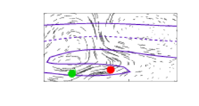
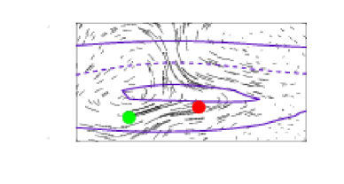
(c)Time = $893.75$	(d)Time = $900$

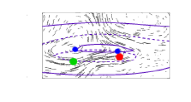
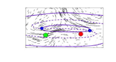
Figure 7: Induced nucleation of dislocations by penta-hepta defects for $\beta=-0.2$ and $\mu=1$. Other parameters as in Fig.4a. Solid lines are zero contour lines for real part of $A_{1}$, and dashed lines for the imaginary part. Grey circles are dislocations in $A_{2}$ and $A_{3}$ and the arrows indicate the mean flow velocity field.

Figure 8: Sketch of defect proliferation by induced nucleation.

The nonlinear gradient terms appear to be central for the induced nucleation in that they lead to a separation of the dislocations making up the penta-hepta defects as is illustrated in Fig.7a. The dependence of the distance between the dislocations on $\alpha_{3}$ is shown in Fig.9. For $\alpha_{3}\geq 0.6$ the PHD becomes unstable through the induced nucleation of dislocations. We find that the dislocations are also separated if only the nonlinear gradient terms corresponding to $\alpha_{1}$ or $\alpha_{2}$ are included (see also [22]). Breaking the chiral symmetry through the $\gamma$-term does not affect the distance between the dislocations in a PHD pair, nor does the mean flow.

Figure 9: Distance between dislocations within a bound PHD as a function of $\alpha_{3}$ for $\beta=0$. Other parameters as in Fig.4.

The stability of the PHD, however, depends not only on the distance between its two constituent dislocations but also on the mean flow. This is shown in Fig.10 where the stability limit of PHDs is given as a function of $\alpha_{3}$ and $\beta$ for a background wavenumber $q=0$. It is obtained by direct numerical simulations of a PHD pair in a system of size $42\times 48$. Note that for this system size there is still a small, but noticeable interaction between the two PHDs that have to be placed in the system to satisfy the periodic boundary conditions. In the stable regime the two PHDs move relatively slowly towards each other and would eventually annihilate each other, whereas in the unstable regime the seeded PHDs nucleate new dislocations and get transformed into different PHDs before they reach each other.

Clearly, increased mean flow greatly facilitates the induced nucleation of dislocations rendering the PHDs much less stable even though the distance of the constituent dislocations is hardly affected by the mean flow. Thus, even relatively small values of $\alpha_{3}$ can be sufficient to induce nucleation if $|\beta|={\mathcal{O}}(1)$. When $\alpha_{3}$ is decreased below $\alpha_{3}\approx 0.1$ the induced nucleation as described above is replaced by a different process in which new dislocations appear not in the previously defect-free mode but in the modes that carry already a dislocation. This is presumably due to the fact that with increasing mean-flow strength the side-band stability limit of the periodic hexagon pattern is shifted further to the left (for example, see Fig.1 in [14]) and comes very close to the background wavenumber $q=0$ employed in Fig.10.

Figure 10: Stability limits of penta-hepta defects (squares) and limit of persistent spatio-temporal chaos (diamonds) as a function of mean-flow strength $\beta$ and of $\alpha_{3}$. Remaining parameters are $\mu=1$, $\nu=2$, $\gamma=0.2$, $\tau=0.5$, and $q=0$.

4.2 Persistent PHD-Chaos

A particularly interesting aspect of the simulations shown in Fig.5b is the fact that the induced nucleation of dislocations is not merely transient as had been the case in [22], but instead persists for the whole duration of the simulation. To bring out the persistence of the dynamics more clearly, we give a detailed analysis of the pattern evolution by measuring the local wavenumber ${\bf q}_{j}({\bf x})$ of each component,

$${\bf q}_{j}({\bf x}) \equiv \Re\left(\frac{-i\vec{\nabla}A_{j}}{A_{j}}\right)\;\;{\mbox{ for $j=1$, $2$, $3$}}.$$ (15)

We extract the spatial average of the transverse and of the longitudinal components $q_{lj}$ and $q_{tj}$ of ${\bf q}_{j}$, respectively,

$$\overline{q_{lj}}=\overline{\hat{n}_{j}\cdot{\mathbf{q}}_{j}}\equiv\frac{\int_{\Gamma}\hat{n}_{j}\cdot{\mathbf{q}}_{j}\;\,d^{2}{\bf x}}{\int_{\Gamma}d^{2}{\bf x}}, \overline{q_{tj}}=\overline{\hat{\tau}_{j}\cdot{\mathbf{q}}_{j}}\equiv\frac{\int_{\Gamma}\hat{\tau}_{j}\cdot{\mathbf{q}}_{j}\;\,d^{2}{\bf x}}{\int_{\Gamma}d^{2}{\bf x}}.$$ (16)

Here $\Gamma$ denotes the spatial domain. Figs.11a,b show the temporal evolution of the two wave-vector components corresponding to the evolution of the number of defects shown in Figs.5a,b (for system size $42\times 48$). The rapid initial change in both components corresponds to the period in time when the long-wave instability first generates dislocations. For all three values of $\beta$ the longitudinal component rapidly relaxes to a very small value near $\overline{q_{li}}=0$ and, with the exception of small fluctuations, stays there for the whole duration of the simulations. Similarly, for $\beta=0$ the transverse component reaches in a somewhat slower transient a stationary value of $\overline{q_{tj}}\approx 1.6$. The resulting reconstructed pattern at the final time $t=2500$ is shown in Fig.12a. It still contains a few PHD, which move very slowly. Compared to the initial pattern, in which the hexagons were aligned with the $x$-axis, the pattern is rotated by a small amount reflecting the change in the average wave-vector, in particular its non-zero transverse component.

Figure 11: Spatially averaged local wave vectors as functions of time: thick lines are the transverse components $\overline{q_{tj}}$ and thin lines are the longitudinal components $\overline{q_{lj}}$ of the wave-numbers. Solid lines are for $A_{1}$, dashed lines for $A_{2}$ and dotted lines for $A_{3}$. Panel (a) is for $\beta=0$ and panel (b) is for $\beta=-0.1$ and $\beta=-0.2$.

For $\beta=-0.1$ and $\beta=-0.2$ the number of PHDs keeps fluctuating throughout the simulation. The corresponding evolution of the average wave-vector is shown in Fig.11b. As is the case for $\beta=0$, during the initial phase of defect generation the longitudinal component relaxes rapidly to $\overline{q_{lj}}=0$ while the transverse component reaches a value of $\overline{q_{tj}}\approx 1$ during that phase. Thereafter, the longitudinal component remains near $0$ whereas the transverse component keeps growing at a rate which increases with decreasing (negative) $\beta$. In the reconstructed pattern, shown in Fig.12b at $t=2500$, this manifests itself in a reduced overall wavelength of the hexagons and, more importantly, an increased rotation of the pattern. Following the reconstructed pattern over time one can see that on average it is steadily rotating in a counter-clockwise fashion.

Figure 12: Reconstructed hexagonal patterns at the end of the simulations ($t=2500$) for $\beta=0$ on the left and $\beta=-0.1$ on the right.

To interpret the evolution shown in Fig.11b it is useful to write $A_{i}({\bf x},t)$ as

$$A_{j}={\mathcal{A}}_{j}({\bf x},t)e^{iq_{t}\hat{\tau}_{j}\cdot{\bf x}},\qquad j=1,2,3.$$ (17)

For constant ${\mathcal{A}}_{j}$ this corresponds to a hexagon with non-vanishing transverse wave-vector components that are equal in all three modes. Insertion of (17) into (1,2) shows that the solution and its stability does not depend on $q_{t}$. In particular, the contributions from $\alpha_{2}$ cancel each other. This independence of $q_{t}$ reflects the isotropy of the underlying physical system and the leading-order approximation of the critical circle by its tangents in the direction of $\hat{\tau}_{j}$ at each of the three critical wave-vectors corresponding to the modes $A_{j}$. This suggests that the steady increase of $\overline{q_{tj}}$ with fixed $\overline{q_{lj}}$ should be interpreted as the representation of a rotation of the physical pattern (at fixed magnitude of the wave-vector) within the approximation of the Ginzburg-Landau equations (1,2). A similar phenomenon had been observed for hexagons with broken chiral symmetry in the absence of mean flow [8]. In that system it had been found that if the operator $\hat{n}_{j}\cdot\nabla$ was replaced by the Newell-Whitehead-Segel operator [23, 24] or by the Gunaratne operator [25] the steady growth of the wave-vector components did not follow $\hat{\tau}_{j}$ but instead followed the respective lines in Fourier space along which the growth rate of perturbations of the basic state is constant within these two different approximations [26].

Given the above discussion, it is appropriate to consider within the approximation (1,2) all hexagon solutions with $q_{lj}=0$ as having a wave-vector at the band-center, with $q_{tj}$ indicating the orientation of the pattern in space. This raises the question why new dislocations are generated persistently even though the background wavenumber is in the band center where the periodic hexagon patterns are linearly stable? In [22] it had been found that without mean flow the PHDs can be unstable even if the wavenumber of the background hexagon pattern is inside the stable band, but away from the band center. As was shown in Fig.10 above, in the presence of mean flow PHDs can be unstable even at the band center. We have not investigated whether there are parameter regimes for which the PHDs are unstable at all background wavenumbers. While instability at the band center is consistent with the persistence of spatio-temporal chaos since the background wavenumber of the chaotic state is $q=0$, it is not sufficient. This is indicated in Fig.10, where also the persistence limit for the chaotic state is shown. Below the squares the PHD’s are unstable but chaos only persists for values of $\beta$ below the diamonds. In the parameter regime between these two lines defects are being created intermittently during the transient towards the stationary state, which leads to fluctuations in the defect number, but the defect creation rate is too small compared to the annihilation rate to sustain the chaos.

To illustrate explicitly how the instability of a PHD at the band center can lead to persistent PHD chaos, we performed simulations that start from hexagons at the band center ($q=0$) with a pair of PHDs as a seed for the nucleation process. The resulting evolution of the number of defects and of the spatially averaged transverse wave-vector component is shown in Figs.13a,b, respectively. Compared to the simulations shown in Fig.12b, the value of $\alpha_{3}$ is reduced to $\alpha_{3}=0.5$. As a consequence even for $\beta=-0.2$ no new dislocations are generated. For $\beta=-0.4$ there is an initial volley of induced nucleation, but eventually the defects annihilate each other again completely. Only for $\beta\leq-0.5$ indications for persistent nucleation are seen. This illustrates that the instability of PHD is not a sufficient condition for persistent chaos; it is necessary that creation balances annihilation for some finite average number of PHDs.

Worth noting is the precipitous decline in the defect number for $\beta=-0.6$ near $t=900$. At that time the transverse wave-vector component reaches values close to the maximal spatial resolution for the number of modes used ($128\times 128$). More detailed studies of the case with $\alpha=0.7$ and $\beta=-0.2$ have shown that if the number of modes is increased the suppression of the induced nucleation is delayed until larger values of $\overline{q_{tj}}$ are reached. Thus, the saturation of $\overline{q_{tj}}$ for $\beta=-0.5$ in Fig.13b and the associated end of the chaotic activity is a numerical artifact. Note, however, that the chaotic defect states reported here have lasted substantially longer than the transient states found in [22].

Figure 13: a) Temporal evolution of number of dislocations for $\alpha=0.5$ and various values of $\beta$. Other parameters as in Fig.5. b) Evolution of the spatially averaged transverse wave vector component $\overline{q_{tj}}$.

Since the defect nucleation persists even for wavenumbers near the band-center it is not surprising that similar chaotic states are reached when the stability limit for periodic hexagons is crossed on the large-$q$ side. It should be noted that in simulations that started from a slightly perturbed hexagon pattern beyond the low-$q$ stability limit no persistent nucleation was found when the wavenumber was too far in the unstable regime. In that case only a very large number of defects was generated in the initial phase, which then quickly annihilated each other.

Of course, the steady increase of the transverse wave-vector component apparent in Fig.11b implies that after a finite amount of time the magnitude of the transverse component $q_{tj}$ becomes of the same order as the critical wavenumber. At that point the Ginzburg-Landau equations clearly will have become invalid, since they are based on the approximation that the amplitudes $A_{j}$ vary only slowly compared to the critical wavelength. We have therefore also simulated a modified Swift-Hohenberg equation that corresponds to the same amplitude equations with coefficients corresponding to the values used in the simulations presented here. As expected, we find that the hexagon pattern keeps rotating on average as the defect proliferation and annihilation continue indefinitely [27].

In general, the other nonlinear gradient terms corresponding to $\alpha_{1}$ and $\alpha_{2}$ have to be taken into account as well. We have performed simulations for selected parameter values of $\alpha_{1}$ and $\alpha_{2}$ that correspond, for instance, to realistic values for surface-tension-driven Bénard-Marangoni convection ($\alpha_{1}=0.3$ and $\alpha_{2}=1.1$, corresponding to a Prandtl number $\sim 10$ in a single-fluid model [28]; $\alpha_{1}=-0.1$ and $\alpha_{2}=0.4$ corresponding to a two-fluid model a water-air layer [29]). While we find induced nucleation even in the absence of rotation and without $\alpha_{3}$, persistent spatio-temporal chaos arises only if $\alpha_{3}\geq 0.8$ in both cases ($\beta=-0.2$).

5 Effects of non-linear gradient terms on PHD motion

The motion of individual PHD’s within the lowest-order Ginzburg-Landau equations has been studied in detail in [30, 31], where in extension of the results for dislocations in roll patterns [32] the dependence of the velocity of a PHD on the background wave-vectors of the three hexagon modes has been determined semi-analytically. The effect of the mean flow on the defect motion has been discussed in some detail in [14]. Here we turn to the impact of the other non-variational terms, specifically the non-linear gradient terms, on the motion of the PHD’s.

In our analysis we closely follow the approach of [31]. We factor out the background wave-vectors of the three hexagon modes by writing $A_{j}\equiv a_{j}e^{i{\bf q}_{j}\cdot{\bf x}}$. Assuming a constant defect velocity ${\mathbf{V}}$, the time derivative in (1) is replaced by $-{\mathbf{V}}\cdot\nabla$. We then project (1) onto the two translation modes, i.e. for each $j$ we multiply (1) by $\partial_{x}a_{j}^{*}$ and $\partial_{y}a_{j}^{*}$, respectively, and add all three equations and their complex conjugates. The resulting projection can be written as

$$I_{xx}V_{x}+I_{xy}V_{y}=F, I_{yx}V_{x}+I_{yy}V_{y}=G,$$ (18)

where the components of the mobility tensor are given by

$$I_{xx}\equiv \left<\sum_{i=1}^{3}|\partial_{x}a_{i}|^{2}\right>,\;\;I_{yy}\equiv\left<\sum_{i=1}^{3}|\partial_{y}a_{i}|^{2}\right>,$$

$$I_{xy}= I_{yx}=\frac{1}{2}\left<\sum_{i=1}^{3}\partial_{x}a_{i}\partial_{y}a_{i}^{*}+c.c.\right>,$$ (19)

and $<\cdots>\equiv\int\int\cdots dxdy$ denotes the integral over the domain. The terms on the right-hand-side of equation (1) contribute to $F$ and $G$ with

$$F = -2\gamma\left<\sum_{i=1}^{3}|a_{i}|^{2}\partial_{x}|a_{i+1}|^{2}\right>-i\left<\sum_{i=1}^{3}q_{i}\partial_{x}a_{i}^{*}(\hat{n}_{i}\cdot\nabla)a_{i}-c.c.\right>$$ (20)

$$-i\frac{\beta}{2}\left<\sum_{i=1}^{3}\partial_{x}a_{i}^{*}a_{i}(\hat{\tau}_{i}\cdot\nabla)Q-c.c.\right>$$

$$-i\frac{\alpha_{1}}{2}\left<\sum_{i=1}^{3}\partial_{x}a_{i}^{*}\left[a_{i-1}^{*}(\hat{n}_{i+1}\cdot\nabla)a_{i+1}^{*}+a_{i+1}^{*}(\hat{n}_{i-1}\cdot\nabla)a_{i-1}^{*}\right]-c.c.\right>$$

$$-i\frac{\alpha_{2}}{2}\left<\sum_{i=1}^{3}\partial_{x}a_{i}^{*}\left[a_{i-1}^{*}(\hat{\tau}_{i+1}\cdot\nabla)a_{i+1}^{*}-a_{i+1}^{*}(\hat{\tau}_{i-1}\cdot\nabla)a_{i-1}^{*}\right]-c.c.\right>$$

$$-i\frac{\alpha_{3}}{2}\left<\sum_{i=1}^{3}\partial_{x}a_{i}^{*}\left[a_{i-1}^{*}(\hat{n}_{i+1}\cdot\nabla)a_{i+1}^{*}-a_{i+1}^{*}(\hat{n}_{i-1}\cdot\nabla)a_{i-1}^{*}\right]-c.c.\right>$$

$$\equiv \gamma F_{\gamma}+q_{0}F_{q}+\beta F_{\beta}+\alpha_{1}F_{1}+\alpha_{2}F_{2}+\alpha_{3}F_{3}.$$

$G$ is defined analogously to $F$ with $\partial_{x}a_{i}^{*}$ in front of the square brackets in each of the integrals replaced by $\partial_{y}a_{i}^{*}$. The projection $q_{i}$ of the wave-vector ${\bf q}$ onto ${\hat{n}}_{i}$ is given by $q_{i}={\bf q}_{i}\cdot{\hat{n}}_{i}$. To leading order the transverse components ${\bf q}_{i}\cdot\hat{\tau}_{i}$ of the wave-vectors do not affect the velocity of the defect. Here we only focus on situations where $q_{i}\equiv q_{0}$ is the same for all three amplitudes. Note, that the other terms in (1) do not contribute to (20), which can be seen by integrating by parts and using the appropriate boundary conditions.

In the absence of the non-potential terms ($\gamma=\beta=\alpha_{1}=\alpha_{2}=\alpha_{3}=0$) the PHD is stationary for $q_{0}=0$ and the two dislocations making up the PHD are located at the same position. Without loss of generality, we assume that the PHD consists of a pair of dislocations in $A_{2}$ and $A_{3}$. Treating the non-potential terms perturbatively it is sufficient to use the potential solution for the stationary defect to evaluate the inhomogeneous terms $F$ and $G$. Far away from the defect core the pattern is well described by the phase equations; rewriting the demodulated amplitude as $a_{j}=\rho_{j}(r,\phi)e^{i\theta_{j}(r,\phi)}$, where $r$ is the radial distance from the defect core and $\phi$ is the azimuthal angle around the core, one obtains then [33] $\rho_{i}(r\rightarrow\infty,\phi)\rightarrow\rho_{0}$ and

$$\theta_{1} = \frac{1}{2\sqrt{3}}(1-\cos(2\phi)),$$ (21)

$$\theta_{2} = \phi-\frac{1}{2\sqrt{3}}\left[\frac{1}{2}+\cos(2\phi-\frac{2\pi}{3})\right],$$ (22)

$$\theta_{3} = -\phi-\frac{1}{2\sqrt{3}}\left[\frac{1}{2}+\cos(2\phi+\frac{2\pi}{3})\right].$$ (23)

This solution is utilized for the far-field contribution to the integrals for $F$ and $G$. The numerical solution of the Ginzburg-Landau equation (1,2) is used for the evaluation of the integral in the core region. It can be shown that the far-field contribution to the integrals $G_{1}$, $G_{2}$, and $F_{3}$ is zero, while that to the integrals $F_{1}$, $F_{2}$, and $G_{3}$ is non-zero. For example, for $G_{1}$ the angular integral involving $\theta_{1}$ vanishes, and those involving $\theta_{2}$ and $\theta_{3}$ cancel each other, leading to a vanishing contribution to $G_{1}$ from the far field. Numerically, we also found that the core integrals for $G_{1}$, $G_{2}$, and $F_{3}$ vanish; they are at least $100$ times smaller than the core integrals for $F_{1}$, $F_{2}$, and $G_{3}$. In the following we ignore $F_{\gamma}$ and $G_{\gamma}$; similar to the integrals $G_{1}$, $G_{2}$, and $F_{3}$, the integrals $F_{\gamma}$ and $G_{\gamma}$ vanish in the far-field and amount to very small values when evaluated numerically around the core. Thus, we conclude that to leading order in the non-potential terms (and the wavenumber $q_{0}$) the velocity of an individual PHD is well approximated by

$$\left(\begin{array}[]{cc}I_{xx}&I_{xy}\\ I_{yx}&I_{yy}\end{array}\right)\left(\begin{array}[]{c}V_{x}\\ V_{y}\end{array}\right) = q\left(\begin{array}[]{c}F_{q}\\ G_{q}\end{array}\right)+\beta\left(\begin{array}[]{c}F_{\beta}\\ G_{\beta}\end{array}\right)+\left(\begin{array}[]{c}\alpha_{1}F_{1}+\alpha_{2}F_{2}\\ \alpha_{3}G_{3}\end{array}\right).$$ (34)

To evaluate the mobility tensor on the left-hand side of (34) it is not sufficient to insert the solution for the stationary defect in (5) since it leads to integrals that diverge in the far field. To regularize this singularity the solution for the moving defect has to be used, at least in the far field [34, 32, 31]. To leading order, the non-potential terms can be neglected in the mobility tensor. Then its off-diagonal terms are much smaller than the diagonal terms [31]. Using the numerically determined defect solution of the full equations (1,2), we also find $I_{xy}$ to be much smaller than either $I_{xx}$ or $I_{yy}$ (by a factor of $100$) when we only compute the integral within a box enclosing the defect core and neglect the far-field contribution.

The effect of the non-linear gradient terms can now be summarized as follows: since the off-diagonal terms in the mobility tensor are small, the contributions of $\alpha_{1}$ and $\alpha_{2}$ to the velocity of a PHD with dislocations in amplitudes $A_{2}$ and $A_{3}$ are in the $\hat{n}_{1}$-direction (“glide”), while $\alpha_{3}$ causes such a PHD to travel in the ${\hat{\tau}}_{1}$-direction (“climb”). Furthermore, like the mean flow the nonlinear gradient terms contribute to a shift of the wavenumber at which the defect is stationary away from the band center $q=0$.

The above conclusion is confirmed in direct numerical simulations of (1,2). In Fig.14 we plot the velocity of a PHD with charges $(0,-,+)$ for $\mu=1$, $q_{0}=0$, $\gamma=0.2$, and $\beta=0$ as a function of the strength of the nonlinear gradient terms. As expected from the discussion of (34), if only $\alpha_{1}$ or $\alpha_{2}$ are non-zero the defect glides, whereas it climbs if only $\alpha_{3}$ is present. The velocities change sign if the charges of the PHD are reversed.

Figure 14: Defect velocity due to $\alpha_{1,2}$ (glide) and due to $\alpha_{3}$ (climb), respectively, for $q_{0}=0$, $\mu=1$, $\gamma=0.2$, $\beta=0$, and $\nu=2$.

Figure 15: Dependence of the defect velocity on the wavenumber $q$ for $\mu=1$, $\nu=2$ and $\beta=0$. $\alpha_{i}=0$ except as indicated: $\alpha_{1}=0.3$ (circles), $\alpha_{2}=0.3$ (triangles), $\alpha_{3}=0.3$ (squares). Dotted line is for the variational case $\alpha_{1}=\alpha_{2}=\alpha_{3}=0$.

Fig.14 indicates that the linear dependence of the velocity on the $\alpha_{i}$ is restricted to a range $|\alpha_{i}|\leq 0.2$. It is found, however, that the direction of the defect motion remains the same for $\alpha_{i}$ outside that range, i.e. $\alpha_{1}$ and $\alpha_{2}$ cause defects to glide while defects climb due to $\alpha_{3}$. In comparison, in previous numerical simulations we found that the mean flow causes the PHD’s to perform a combined climb-glide motion [14]. This indicates that both $F_{\beta}$ and $G_{\beta}$ are non-zero in equation (34). Fig.15 shows the dependence of the defect velocity on the wavenumber $q$. For $\alpha_{3}\neq 0$, the defect performs a mixed climb-glide motion if the wave number is not at the band center, i.e. if $q\neq 0$.

6 Conclusion

The variational character of the minimal Ginzburg-Landau equations for steady hexagon patterns can be broken in various ways. Quite generally, at cubic order two nonlinear gradient terms arise [35, 36]. If the chiral symmetry of the system is broken (e.g. by rotation) a third nonlinear gradient term is possible [8]. In Rayleigh-Bénard and in Marangoni convection the mean flow driven by deformations of the pattern introduce a further non-variational term in the form of a non-local coupling of the roll modes (e.g. [16, 37]). In this paper we have studied the combined effect of the mean flow and of rotation (including the respective nonlinear gradient term) on the stability and dynamics of hexagon patterns as well as on the stability and motion of their penta-hepta defects.

Rotation induces a coupling of the two long-wave phase modes that can generate a long-wave oscillatory instability, which in the absence of nonlinear gradient terms is, however, usually screened by a steady short-wave instability [8]. The mean flow is only driven by the transverse phase mode [14]. Our results indicate that it suppresses the rotation-induced coupling of the phase modes that leads to oscillatory behavior.

The various non-variational terms influence the motion of penta-hepta defects in different ways. While the nonlinear gradient terms that preserve the chiral symmetry contribute to a gliding motion of the defects, the nonlinear gradient term introduced by rotation induces a climbing motion. This is to be contrasted with the effect of the mean flow, which leads to a mixed climbing-gliding motion.

The most interesting result of this paper is associated with the fact that the nonlinear gradient terms lead to a separation of the two dislocations making up a penta-hepta defect and can destabilize it [22]. More specifically, in simulations we find that penta-hepta defects induce the nucleation of new dislocations in the defect-free amplitude. Even a weak mean flow can enhance this instability significantly. Moreover, with a sufficiently strong nonlinear gradient term that breaks the chiral symmetry ($\alpha_{3}$) the induced nucleation can lead to an ever-increasing transverse wavevector component of the hexagon patterns. As in the case without mean flow [8], we interpret this growth, which eventually leads to the break-down of the Ginzburg-Landau equations, as the signature of a persistent precession of the disordered pattern on average. In Fourier space, the wave-vector spectrum of such a precessing pattern would drift along the critical circle. In the lowest-order Ginzburg-Landau equations used here the critical circle is replaced by its tangents at each of the three modes making up the hexagons, which are transverse to the respective wave-vectors. We expect therefore that in this regime the physical system would exhibit persistent penta-hepta defect chaos driven by induced nucleation.

To overcome the limitations of the Ginzburg-Landau equations, we are currently investigating penta-hepta defect chaos using a suitably modified Swift-Hohenberg-type equations coupled to a mean flow [27]. As expected from the simulations of the Ginzburg-Landau equations presented in the present paper, the penta-hepta defect chaos persists and on average the disordered hexagon patterns precess indefinitely. As in the Ginzburg-Landau case, the chaotic state is due to the induced nucleation of penta-hepta defects, which is apparently only possible when the nonlinear gradient terms are included. These simulations also indicate that the induced nucleation is not contingent on the oscillatory sideband instability; rather it is the separation of the dislocations in a penta-hepta defect that renders them unstable and induces the nucleation. To obtain persistent chaos the resulting defect proliferation has to be strong enough compared to the annihilation rate and apparently the chiral symmetry has to be broken.

We wish to acknowledge useful discussion with A. Golovin, A. Nepomnyashchy, and L. Tsimring. This work is supported by the Engineering Research Program of the Office of Basic Energy Sciences at the Department of Energy (DE-FG02-92ER14303), by a grant from NASA (NAG3-2113), and by a grant from NSF (DMS-9804673). YY acknowledges computation support from the Argonne National Labs and the DOE-funded ASCI/FLASH Center at the University of Chicago.

References

- [1] S. Morris, E. Bodenschatz, D. Cannell, and G. Ahlers, Phys. Rev. Lett. 71, 2026 (1993).
- [2] G. Küppers and D. Lortz, J. Fluid Mech. 35, 609 (1969).
- [3] F. Zhong, R. Ecke, and V. Steinberg, Physica D 51, 596 (1991).
- [4] Y. Hu, W. Pesch, G. Ahlers, and R. E. Ecke, Phys. Rev. E 58, 5821 (1998).
- [5] K. Nitschke and A. Thess, Phys. Rev. E 52, 5772 (1995).
- [6] M. Schatz et al., Phys. Rev. Lett. 75, 1938 (1995).
- [7] E. Bodenschatz, J. R. deBruyn, G. Ahlers, and D. Cannell, Phys. Rev. Lett. 67, 3078 (1991).
- [8] B. Echebarria and H. Riecke, Physica D 139, 97 (2000).
- [9] A. M. Mancho, H. Riecke, and F. Sain, Chaos (accepted).
- [10] F. Sain and H. Riecke, Physica D 144, 124 (2000).
- [11] J. Swift, in Contemporary Mathematics Vol. 28 (American Mathematical Society, Providence, 1984), p. 435.
- [12] A. Soward, Physica D 14, 227 (1985).
- [13] B. Echebarria and H. Riecke, Phys. Rev. Lett. 84, 4838 (2000).
- [14] Y.-N. Young and H. Riecke, Physica D 163, 166 (2002).
- [15] M. Sushchik and L. Tsimring, Physica D 74, 90 (1994).
- [16] E. Siggia and A. Zippelius, Phys. Rev. Lett. 47, 835 (1981).
- [17] S. M. Cox and P. C. Matthews, J. Fluid Mech. 403, 153 (2000).
- [18] A. Nuz et al., Physica D 135, 233 (2000).
- [19] B. Echebarria and H. Riecke, Physica D 143, 187 (2000).
- [20] R. Hoyle, Appl. Math. Lett. 8, 81 (1995).
- [21] B. Echebarria and C. Pérez-García, Europhys. Lett. 43, 35 (1998).
- [22] P. Colinet, A. A. Nepomnyashchy, and J. C. Legros, Europhys. Lett. (2002).
- [23] A. Newell and J. Whitehead, J. Fluid Mech. 38, 279 (1969).
- [24] L. Segel, J. Fluid Mech. 38, 203 (1969).
- [25] G. Gunaratne, Q. Ouyang, and H. Swinney, Phys. Rev. E 50, 2802 (1994).
- [26] B. Echebarria and H. Riecke, unpublished .
- [27] Y.-N. Young and H. Riecke, in preparation .
- [28] J. Bragard and M. G. Velarde, J. Fluid Mech. 368, 165 (1998).
- [29] A. Golovin, A. Nepomnyashchy, and L. Pismen, J. Fluid Mech. 341, 317 (1997).
- [30] L. Tsimring, Phys. Rev. Lett. 74, 4201 (1995).
- [31] L. Tsimring, Physica D 89, 368 (1996).
- [32] E. Bodenschatz, W. Pesch, and L. Kramer, Physica D 32, 135 (1988).
- [33] L. M. Pismen and A. A. Nepomnyashchy, Europhys. Lett. 24, 461 (1993).
- [34] E. Siggia and A. Zippelius, Phys. Rev. A 24, 1036 (1981).
- [35] H. Brand, Prog. Theor. Phys. Suppl. 99, 442 (1989).
- [36] E. A. Kuznetsov, A. A. Nepomnyashchy, and L. M. Pismen, Phys. Lett. A 205, 261 (1995).
- [37] A. Golovin, A. Nepomnyashchy, and L. Pismen, Physica D 81, 117 (1995).