Individual-based lattice model for spatial spread of epidemics

1 Introduction

Since the publication of Kermack and McKendrick epidemic model [1] in 1927, mathematical epidemiology developed an extensive body of literature. A vast majority of proposed models, to study dynamics of epidemics, is based on ordinary differential equations. These models assume that the population mixing is strong, hence concentrations of effected types of population (for example, susceptible, infected, removed) are spatially homogeneous. Thus, these models neglect spatial aspects of the epidemic process. Models which rely on partial differential equations, such as [2], abandon the assumption of homogeneous mixing and allow to study the geographical spread of epidemics, yet they still pose some serious problems. They treat the population as continuous entity, and neglect the fact that populations are composed of single interacting individuals. This can lead to very unrealistic results, such as, for example, endemic patterns relaying on very small densities of individuals, named in [3] “atto-foxes” and “nano-hawks”.

Models based on interacting particle systems eliminate these shortcomings of traditional methodologies. They treat individuals in biological populations as discrete entities, allow to introduce local stochasticity, and are well suited for computer simulations. Several models of this type have been suggested in a recent decade, including stochastic interacting particle models [4], and models based on cellular automata or coupled map lattices [5, 6, 7, 8, 9].

In this article, we present lattice gas cellular automaton (LGCA) for SIR (susceptible-infected-removed) type of an epidemic. Our aim is to demonstrate that the LGCA approach provides an interesting and potentially fruitful alternative to other methods. In real biological populations, both animal and human, contact processes among infectious and susceptible individuals and their movement play a vital role in spreads of epidemics of an infectious disease. Infectious diseases spread because infectious and susceptible individuals mix together. They move, meet each other and through a contact process they transmit an infection. Hence, among other factors the spread of infectious diseases strongly depends on patterns of mobility in populations. In LGCA, population mixing arises directly from motion of individuals and susceptible individuals can become infected only if they meet infectious individuals. Additionally, a LGCA allows to investigate effects of spatial inhomogeneities in population concentrations on the dynamics of epidemic processes and vaccination strategies. We will demonstrate examples of such effects. In this article we do not aim to construct a LGCA of a particular disease but rather we want to study generic features of LGCA methodology and its suitability in the context of epidemiology. To illustrate the ideas and discuss further possible developments we selected SIR (susceptible-infected-removed) epidemic type for which we constructed a LGCA. We derived approximate mean-field type description of the automaton and simulated and analyzed the automaton dynamics. We compared the predictions obtained from the mean-field description with those obtained from the automaton simulations. Additionally, we used automaton to study various vaccination strategies.

2 Individual-based SIR model on a lattice

We will construct a LGCA for an epidemic of SIR type, for which we can assume that a population consists of three types of moving and interacting individuals, of type $\tau\in\{S,I,R\}$, susceptible, infected, and recovered. The proposed automaton is a special case a lattice gas cellular automaton for reaction-diffusion systems, described in detail in [10, 11].

We tile the physical space, in which an epidemic takes place, by regular hexagonal cells $h(\mathbf{r)}$ with centers at discrete space variables $\mathbf{r}$. We chose the hexagonal cells in order to avoid spurious invariants in the dynamics of the automaton, also known as parity problem [10, 11]. However, other types of tiling, such as square cells, can be used as well. We assume that the distance between centers of adjacent cells is $1.$ Let

$$\mbox{\boldmath$c$}_{i}=<\cos(i-1)\pi/3,\sin(i-1)\pi/3>$$ (1)

be a unit vector, for each $i=1,...,6.$ If we connect the center of every hexagon $h(\mbox{\boldmath$r$})$ with the centers of the neighbouring hexagons $\mbox{\boldmath$r$}+\mbox{\boldmath$c$}_{i}$, where $i=1,...,6,$ then we obtain a hexagonal lattice structure $\mathcal{L}_{h}$, with the lattice coordination number $m=6.$ In the case of square cells the lattice coordination number would be $m=4.$ Figure 1 (reproduced from [12]) shows that the

Figure 1: The array of hexagonal cells with a dashed lattice superimposed on it. The lattice depicts the channels through which the individuals are transported from cell to cell. The figure is reproduced from [12].

centers of the hexagons $h(\mbox{\boldmath$r$})$ become the nodes of the hexagonal lattice $\mathcal{L}_{h}.$ The cells represent some area of the physical space in which the individuals mixed, interact and can move from one place (cell) to another. The individuals can move among the cells only along the channels corresponding to edges of the lattice $\mathcal{L}_{h}.$ Except where confusion might arise, we will identify a cell $h(\mbox{\boldmath$r$})$ with its center $r$, hence with the node $r$ of the lattice $\mathcal{L}_{h}.$ Hence, we can say that the individuals reside at the nodes of the lattice and move along its edges (channels). While extensions to arbitrary boundary conditions are straightforward, we limit our considerations to periodic boundary conditions.

At the initial time, $k=0,$ particles representing individuals $S,$ $I$ and $R$ are distributed randomly and independently, among the cells $h(\mbox{\boldmath$r$}),$ $\mbox{\boldmath$r$}\in\mathcal{L}_{h},$ according to probabilities given by their initial concentrations. The initial distribution of particles is such that there are at most six particles, regardless of the individual type, per cell $h(\mbox{\boldmath$r$})$ (four when the cells are squares). The LGCA discrete dynamics is constructed in such a way that the total number of individuals at a given node is restricted to stay between $0$ and $m$ ($m=6$ or $4$, respectively, for hexagonal or square lattice) per each cell during the time evolution of the automaton. Since a single lattice node represents a small region of space, this means that $m$ can be interpreted as the carrying capacity of that region. In other words, the number of individuals that this region can support cannot exceed $m$.

The time evolution of the automaton takes place at discrete time steps. At each time step $k$, an evolution operator $\mathcal{E}$ is applied, simultaneously and independently of the past, to all lattice nodes. The evolution operator $\mathcal{E}$ governs the dynamics of the automaton, which arises from sequential applications of the three basic operations contact $\mathcal{C}$, randomization $\mathcal{R}$ and propagation $\mathcal{P}$. Hence, the evolution operator can be written in terms of these operations as the superposition

$$\mathcal{E}=\mathcal{P\circ R\circ C}.$$ (2)

Each of the operations $\mathcal{C}$, $\mathcal{R}$ and $\mathcal{P}$ captures some aspects of the epidemic process and their actions are described as follows.

1. As a result of an application of the contact operation $\mathcal{C}$, individuals can change their type, meaning that susceptible individuals can become infected, and infected individuals can recover. More precisely, each susceptible individual at a node $\mathbf{r}$, independently of other individuals, can become infected with probability $1-(1-r)^{n_{I}}$, where $n_{I}$ is a number of infected individuals at the node $\mathbf{r}$, and $r\in[0,1]$. Similarly, each infected individual at the node $\mathbf{r}$, independently of other individuals, can recover with probability $a$, where $a\in[0,1]$.

2. As a result of using the randomization operation $\mathcal{R}$, applied at each node independently of the other nodes, a population of individuals residing at a node $\mathbf{r}$ is randomly redistributed among edges/channels originating from the node $\mathbf{r}$. Through the selected channels, allowing at most one individual per channel, individuals will move in the propagation step from the node $\mathbf{r}$ to the neighbouring nodes. The process of redistribution of individuals is purely probabilistic one and it contributes to modeling the mixing process of individuals.

3. In the propagation step, governed by the operator $\mathcal{P}$, individuals simultaneously move from their nodes to the neighbouring ones through the channels assigned to them in the randomization step. The movement of individuals is purely deterministic in the propagation step.

The rationale behind the probability of becoming infected in the first step being $1-(1-r)^{n_{I}}$ can be explained as follows. We assume that, at a given node, a susceptible individual contacts all infected individuals at that node and that all infected individuals are infectious one. If the probability of infection per contact is $r$, then the probability of not getting infected after contacting each of $n_{I}$ infected individuals is $(1-r)^{n_{I}}$. The probability of getting infected, therefore, is $1-(1-r)^{n_{I}}$.

Note that the mechanism of contracting an infection described here implies that the incubation period is short enough to be negligible, meaning that a susceptible who contracts the disease at time $k$ becomes infectious immediately, and can infect others at time $k+1$. While this is a convenient assumption, it will have to be relaxed in more realistic models, or in models tailored for a specific disease. Also, note that the duration of the disease (number of time steps from contracting an infection to recovery) has geometrical distribution with a mean value of $1/a$ time steps. Again, in realistic disease-specific models a different distribution will have to be adopted, depending on the particular disease. As we said earlier the spread of infectious diseases strongly depends on mixing patterns in the populations. In the LGCA that is being presented here, mixing is of diffusive type. It arises from randomization of directions of motion of individuals in the randomization step $\mathcal{R}$ and the movement of individuals in the propagation step $\mathcal{P}$. In the more realistic models the movement of individuals will have to be appropriately modified and additionally, we will have to include inflow, outflow, birth and death processes.

3 Mean-field approximation

In order to gain some insight into the dynamics of the LGCA defined in the previous section, we will now proceed to construct approximate equations describing the automaton dynamics. Using the formalism and methodology introduced in [11], it is possible to write compact microdynamical equations corresponding to the evolution operator $\mathcal{E}$. Moreover, by making appropriate approximations, it is possible to derive the LGCA discrete lattice-Boltzmann equations and the corresponding partial differential equations describing the automaton macroscopic dynamics. Since rigorous derivation of these equations is rather involved, we refer the interested reader to [11]. We take here a less rigorous, but more intuitive approach.

Let us assume that the total number of nodes in the lattice $\mathcal{L}_{h}$ is $N$, and at time $k$ there are $N_{S}(k)$ susceptible, $N_{I}(k)$ infected, and $N_{R}(k)$ recovered individuals on the entire lattice. Since we do not allow for inflow, outflow, birth and death processes, the total population, denoted by $N_{tot},$ remains constant in time. Define $n_{\tau}(\mathbf{r},k)$ to be a number of individuals of type $\tau$ at a node $\mathbf{r}$ at time $k$. If we assume that the automaton dynamics is spatially homogeneous (well stirred), then the expected value of $n_{\tau}(\mathbf{r},k)$ is independent of $\mathbf{r}$ and equals

$$\langle n_{\tau}(\mathbf{r},k)\rangle=\frac{N_{\tau}(k)}{N}.$$ (3)

Under the same assumptions, regardless at which cell the susceptible individual is located, the expected number of infected individuals at his cell is $N_{I}/N$, thus the probability that he becomes infected is

$$1-(1-r)^{N_{I}(k)/N}.$$ (4)

Hence, the expected number of susceptible individuals who become infected in a single time step is equal to

$$N_{S}(k)[1-(1-r)^{N_{I}(k)/N}].$$ (5)

Similarly, the expected number of individuals who become recovered in a single time step is $aN_{I}(k)$. When the population is well stirred this yields that the expected number of individuals of each type $\tau\in\{S,I,R\}$ at time $k+1$ is

$$N_{S}(k+1) = N_{S}(k)(1-r)^{N_{I}(k)/N},$$

$$N_{I}(k+1) = N_{I}(k)+N_{S}(k)[1-(1-r)^{N_{I}(k)/N}]-aN_{I}(k),$$ (6)

$$N_{R}(k+1) = N_{R}(k)+aN_{I}(k).$$

For small $r$, taking Taylor expansion

$$(1-r)^{N_{I}(k)/N}=1-\frac{rN_{I}}{N}+\frac{N_{I}(N_{I}-N)r^{2}}{2N^{2}}+\ldots,$$ (7)

and by keeping only the first two terms and defining $\rho_{\tau}(k)=N_{\tau}(k)/N$, we obtain

$$\rho_{S}(k+1) = \rho_{S}(k)-r\rho_{S}(k)\rho_{I}(k),$$

$$\rho_{I}(k+1) = \rho_{I}(k)+r\rho_{S}(k)\rho_{I}(k)-a\rho_{I}(k),$$ (8)

$$\rho_{R}(k+1) = \rho_{R}(k)+a\rho_{I}(k).$$

The above equations are quite similar in their structure to the ordinary differential equations obtainable from the classic Kermack-McKendrick model, as described, for example, in [13]. The similarity lies in the fact that the gain in the class of infected individuals occurs at a rate proportional to the density of infectives and susceptibles, in analogy to the mass action law in chemical kinetics. Of course, this is valid only for small values of $r$ and under the assumption of strong mixing, which is not always realistic.

In reality, the epidemic process spreads quite differently than the mean-field approximation (3) predicts. Figure 2 compares the number of infected individuals as a function of time as observed in the LGCA simulations with the mean-field approximation (3). The simulations have been performed on a hexagonal lattice with $10^{4}$ nodes, using $r=0.3$, $a=0.2$. The initial configuration consisted of $16000$ susceptibles and $100$ infected individuals for each simulation. At the initial time for each simulation the individuals were randomly and uniformly distributed on the lattice. The simulation curve in Figure 2 represents average over 50 experiments. The mean-field approximation (MFA) predicts much faster initial spread than observed in the LGCA simulations. This can be easily explained by realizing that the MFA assumes perfect mixing, meaning that an infected individuals can always infect some susceptibles residing at their node. In simulations, since the mixing is limited, it often happens that the number of infected individuals in the vicinity of an infected individuals is larger than average and, similarly, the number of susceptibles is smaller than average. Or, in other words, infected individuals are often grouped together in small regions of space, while in other spatial regions there are no infected individuals at all. Therefore, the effective force of infection is smaller than predicted by MFA.

Figure 2: Number of infected individuals as a function of time, comparison of LGCA simulation results with the mean-field approximation. The simulation curve represents average of 50 LGCA experiments. Each LGCA simulation has been performed on a hexagonal lattice with $10^{4}$ nodes with $r=0.3$, $a=0.2$, and with $16000$ susceptibles and $100$ infected individuals uniformly and randomly distributed on the lattice at $k=0$.  

We should also note that the fraction of susceptibles who eventually became infected is $67\%$ for simulations and $94\%$ for mean-field, meaning the epidemic is less severe when the mixing is weaker, even though it lasts longer, as can be seen in Figure 2.

4 Effects of spatial distribution

In order to illustrate the importance of spatial distribution of individuals in spread of epidemics, let us consider the following problem. Let us assume that in some region of space, to be denoted by $A$, several cases of an infectious disease have been reported. In order to limit the spread of the disease, we would like to vaccinate the population. However, we have only $M$ doses of a vaccine at our disposal, where $M$ is less than the number of susceptible individuals in the population. The natural question arises how should these doses be distributed in the population to minimize the severity of the epidemic?

Figure 3: Number of infected individuals as a function of time, under “uniform” and “barrier” vaccination strategies. Each simulation curve represents average of 100 LGCA experiments. For each type of vaccination strategy each simulation has been performed on a hexagonal lattice with $10^{4}$ nodes with $r=0.3$, $a=0.2$, and with $16000$ susceptibles uniformly and randomly distributed on the lattice at $k=0$, and $10$ infectives uniformly and randomly distributed in the circle of radius 20 on the lattice at $k=0$.

To simplify the problem, we assume that the vaccine is immediately effective, therefore vaccinated individuals become members of the recovered group immediately after vaccination. Additionally, we assume that the region $A$ is a circle of radius $20$ on a hexagonal lattice of $10^{4}$ nodes.

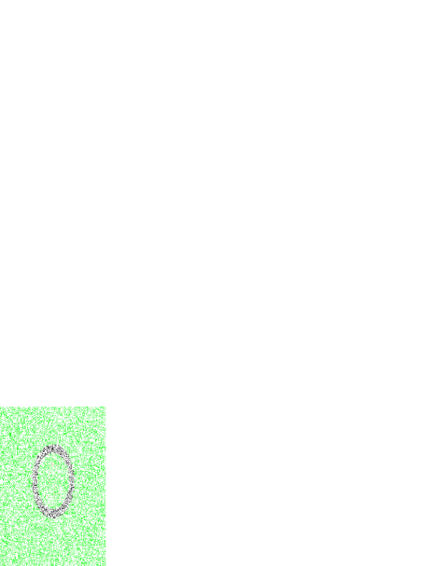
(a)		$k=0$		(e)
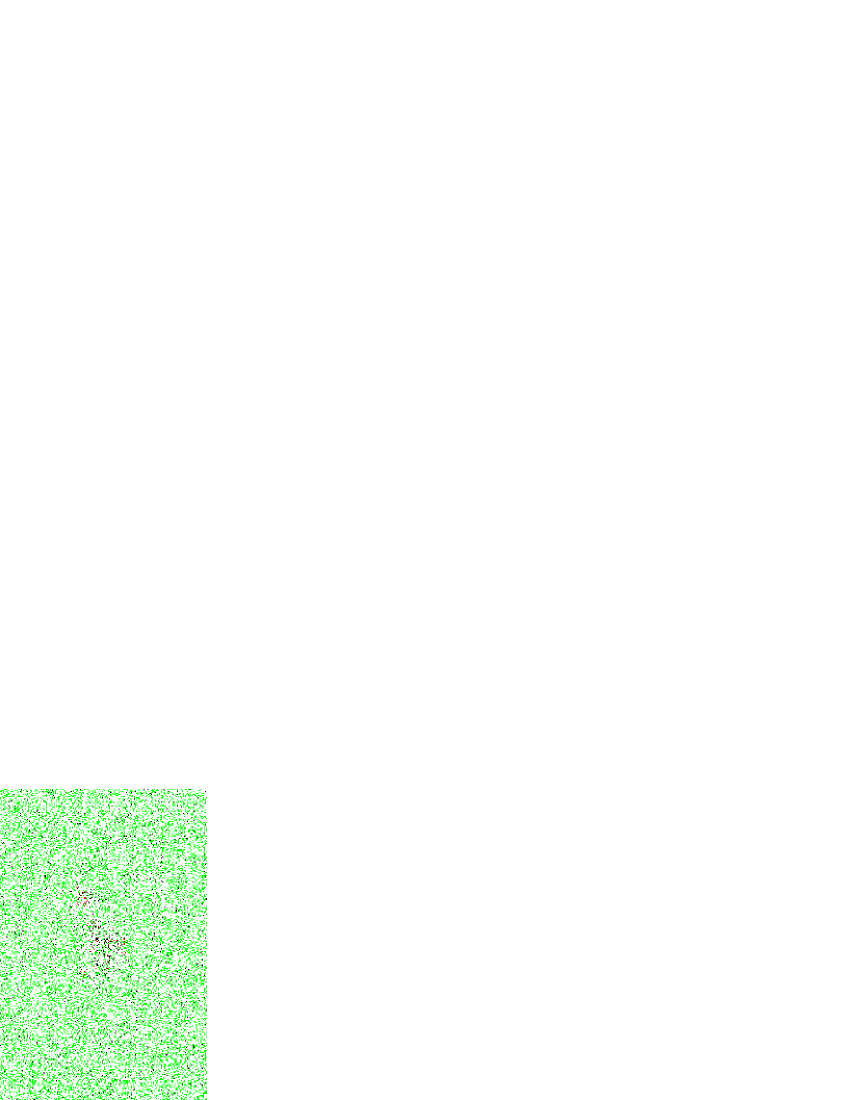
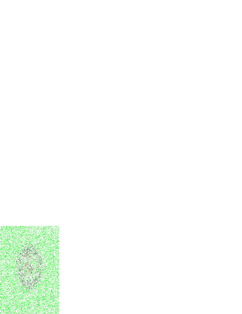
(b)		$k=20$		(f)
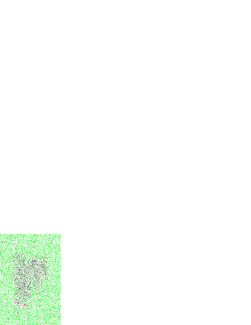
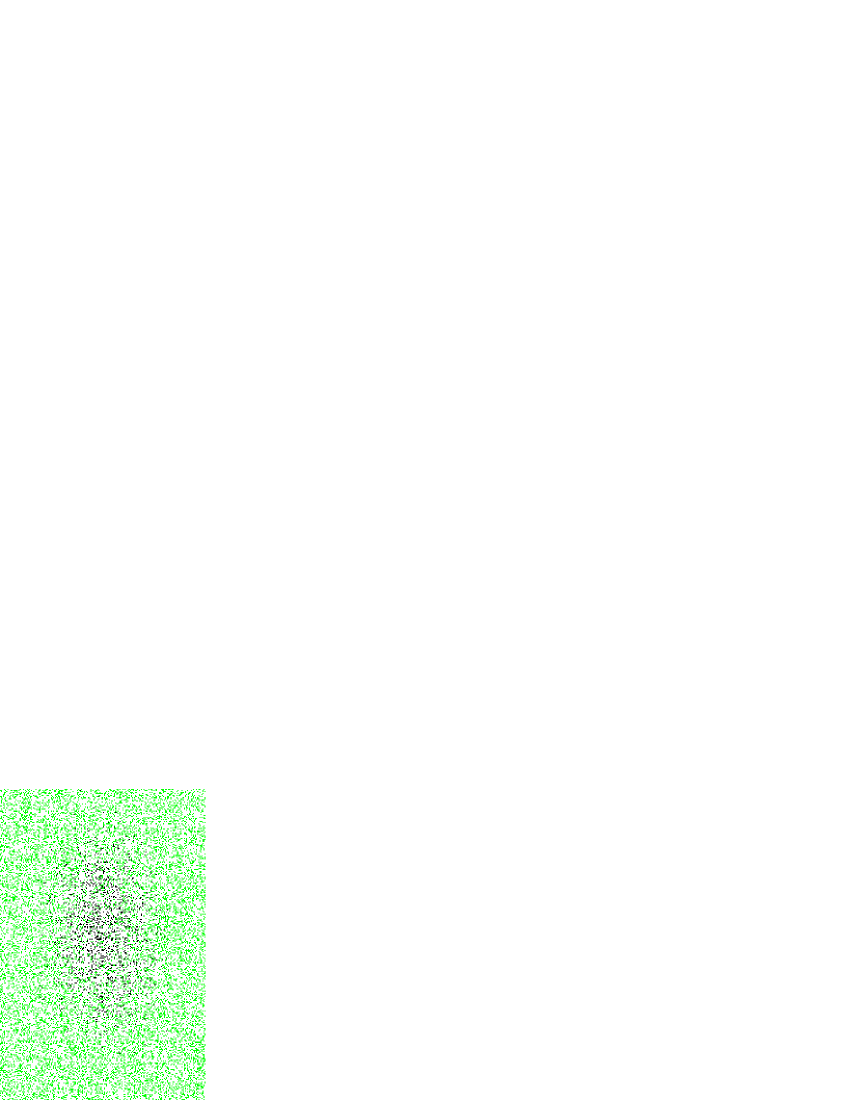
(c)		$k=100$		(g)
(d)		$k=1000$		(h)

Figure 5: Snapshots of LGCA dynamics evolution under “uniform” (left) and “barrier” (right) vaccination strategies.

We compare two alternative vaccination strategies. In the first one, to be referred to as a “uniform strategy”, we vaccinate $M$ individuals selected from the entire population of susceptibles randomly and independently of each other. In the second strategy, to be called a “barrier strategy”, we vaccinate all individuals in a ring surrounding the region $A$. The thickness of the ring is selected in such a way that the total number of vaccinated individuals to be $M$. In all subsequent discussions we assume $M=1000$. Figures 5a and 5e (page 13) show initial distribution of individuals in both these strategies, “uniform” and “barrier”, respectively. Note that the number of individuals in $S$, $I$, and $R$ classes is the same in both cases, so that the spatial distribution of individuals is the only difference between configuration in Figures 5a and 5e. The color coding used is green for $S$, red for $I$, and black for $R$. Consecutive snapshots of the LGCA dynamics in Fig. 5 reveal that the time evolution of these two initial configurations is quite different. One immediately notices that the final configuration in the case of the “uniform” vaccination strategy, after $1000$ time steps (Fig. 5d), contains many more blue pixels than the corresponding final configuration of the “barrier” vaccination strategy (Fig. 5h). This means that many more susceptible individuals contracted the disease in the course of the epidemic when the “uniform” vaccination strategy was used than in the case of the “barrier” vaccination strategy. To be more precise, out of initial $16000$ susceptible individuals out of whom $1000$ have been vaccinated at the start of epidemic, $52\%$ became infected when the vaccination was “uniform”, and only $12\%$ when the “barrier” vaccination strategy was employed. This can be seen from Figure 3, where the number of infected individuals is plotted as a function of time step, averaged over $100$ LGCA experiments.

5 Barrier’s permeability and severity of the epidemics

Figure 4: Average severity of epidemics of an infectious disease $\langle N_{R}(\infty)-N_{R}(0)/N_{tot}\rangle$, calculated as average over severities of outbreaks of epidemics of the disease, as a function of barrier permeability $f$. For each $f$ the average $\langle\cdot\rangle$ has been taken over $100$ LGCA simulations of outbreaks of epidemics, each starting with identical initial configuration, and $r=0.3$ and $a=0.2$.

Since the barrier appears to be a very effective strategy, one could ask how permeability of the barrier influences the dynamics of the epidemics. In what follows, we will vary permeability of the barrier by vaccinating not all susceptibles in the ring surrounding the region $A$, but only a fraction $f$ of randomly selected susceptibles in the ring. Thus, if $f=0$, there is no single vaccinated individual in the ring, while $f=1$ corresponds to the “barrier” described in the previous section, where all susceptibles in the ring are vaccinated.

We define the severity of an outbreak of an epidemic of an infectious disease as $(N_{R}(\infty)-N_{R}(0))/N_{tot}$, where $N_{R}(\infty)$ denotes a total number of removed when a total number of infected in LGCA simulation reaches a steady state and $N_{R}(0)$ denotes the total number of removed (vaccinated individuals) at the start of an epidemic (in an initial configuration in our case). Since in our model we do not allow for birth, death and migration of individuals then the number of removed will remain constant from the moment when the number of infected reaches zero. Let $N_{S}(\infty)$ be a total number of susceptibles at the end of an outbreak of the epidemic. Since $N_{tot}=N_{S}(0)+N_{I}(0)+N_{R}(0)=N_{S}(\infty)+N_{R}(\infty)$, then $N_{R}(\infty)-N_{R}(0)=N_{S}(0)+N_{I}(0)-N_{S}(\infty)$ gives us the total number of susceptibles who got infected in the course of the epidemic. Hence, the average severity of an epidemic of infectious disease can be measured by taking the average $\langle(N_{R}(\infty)-N_{R}(0))/N_{tot}\rangle$ of the severities of outbreaks of specific epidemics of the infectious disease. It tells us on average what chance a susceptible has to become infected in a course of an epidemic. The severity of an epidemic or of an outbreak of the specific epidemic of an infectious disease depends on many factors including the infectivity probability per contact $r$, the recovery probability $a$ and spatial distribution of infected and removed at the outbreak of an epidemic.

In order to examine how the average severity of an epidemic of an infectious disease depends on the barrier permeability we performed a series of simulations varying $f$. For each $f$ we measured the average severity of an epidemic as the average over severities of $100$ epidemic outbreaks each with the infectivity probability per contact $r=0.3$ and the recovery probability $a=0.2$ and strating from the initial conditions described as follows. For each barrier permeability $f$ each simulation has been performed on a hexagonal lattice with $10^{4}$ nodes, and with $10$ infectives uniformly and randomly distributed in the circle $A$ of radius $20$ on the lattice at $k=0$, and with $16000$ susceptibles uniformly and randomly distributed on the lattice, from which in the ring surrounding the circle and consisting of $1000$ susceptibles we “vaccinated”, at $k=0,$ randomly and independently a fraction $f$ of them. Results of this LGCA experiment, which show the average severity of an epidemic of SIR type as a function of barrier permeability $f$ are presented in Figure 4. It is rather remarkable that as $f$ approaches zero, the average severity of an epidemic of SIR type comes close to $49\%$, not much different than the corresponding value for the “uniform” vaccination strategy, when $r=0.3$ and $a=0.2$. This means that the “uniform” vaccination strategy is practically not better than no vaccination at all in this case. Even quite sparse “barrier” is much more effective than uniform random vaccination.

6 Conclusions

We presented a lattice gas cellular automaton for studying spreads of epidemics of SIR type. We derived an approximate mean-field type description of the automaton, and discussed differences between the mean-field approximation and the results of the simulation using LGCA. We also investigated what effects can have spatial inhomogeneities in the distribution of various types of populations on the dynamics of the epidemic process. We demonstrated that the severity of an epidemic can strongly depend of an initial spatial distribution of vaccinated individuals.

The lattice gas cellular automaton discussed in this work is certainly simplistic. It does not take into account many complexities which have to be considered when one attempts to construct a more realistic automaton model for an epidemic. However, the important feature of our model is explicitness of mixing and contact processes. Unlike models based on partial differential equations, our model is individual-based, and the spread of the infection occurs due to the motion of individuals and their interactions. In such models it is quite straightforward to introduce different, non-diffusive type of motion, and investigate the effects of resulting mixing on the dynamics of the epidemic process. For example, we are currently investigating periodic motion with some amount of randomness, that might better represent the behavior of individuals in human populations. Results of such experiments will be presented elsewhere. Here we would like only to reiterate that the description of non-diffusive motion with partial differential equations is usually very difficult or impossible, excluding trivial cases such as linear transport. Individual-based models are much more suitable for this purpose, and we hope that they eventually will help to built epidemic spatial models, tailored for specific diseases, with high degree of realism.

Acknowledgements

H. Fukś and A. T. Lawniczak acknowledge partial support from the Natural Science and Engineering Research Council (NSERC) of Canada, The Fields Institute for Research in Mathematical Sciences, The Mathematics of Information Technology and Complex Systems (MITACS-NCE), and “in-kind” financial support from Nuptek Systems Ltd. The authors thank Bruno Di Stefano for his helpful comments.

References

- [1] W. O. Kermack and A. G. McKendrick, “Contributions to the mathematical theory of epidemics, part I,” Proc. Roy. Soc. Edin. A 115 (1927) 700–721.
- [2] J. D. Murray, E. A. Stanley, and D. L. Brown, “On the spatial spread of rabies among foxes,” Proc. R. Soc. Lond. B 229 (1986) 111–150.
- [3] D. Molisson, “The dependence of epidemic and population velocities on basic parameters,” Math. Biosci. 107 (1991) 255–287.
- [4] R. Durret and S. Levin, “The importance of being discrete (and spatial),” Theoretical Population Biology 46 (1994) 363–394.
- [5] B. Schönfisch, Zelluläre automaten und modelle für epidemien. PhD thesis, Universität Tübingen, 1993.
- [6] N. Boccara and K. Cheong, “Critical behaviour of a probabilistic automata network sis model for the spread of an infectious disease in a population of moving individuals,” J.Phys. A: Math. Gen. 26 (1993) 3707–3717.
- [7] E. Ahmed and H. N. Agiza, “On modeling epidemics, including latency, incubation and variable susceptibility,” Physica A 253 (1998) 347–352.
- [8] M. Duryea, T. Caraco, G. Gardner, W. Maniatty, and B. K. Szymanski, “Population dispersion and equilibrium infection frequency in a spatial epidemic,” Physica D 132 (1999) 511–519.
- [9] A. Benyoussef, N. Boccara, H. Chakib, and H. Ez-Zahraouy, “Lattice three-species models of the spatial spread of rabies among foxes,” Int. J. Mod. Phys. C 10 (1999) 1025–1038.
- [10] J. P. Boon, D. Dab, R. Kapral, and A. T. Lawniczak, “Lattice gas automata for reactive systems,” Physics Reports 273 (1996), no. 2, 55–148.
- [11] A. T. Lawniczak, “From reactive lattice gas automaton rules to its partial differential equations,” Transport Theory and Statistical Physics 29 (2000) 261–288.
- [12] J.-P. Voroney and A. T. Lawniczak, “Construction, mathematical description and coding of reactive lattice-gas cellular automaton,” Simulation Practice and Theory 7 (2000) 657–689.
- [13] J. D. Murray, Mathematical Biology. Springer-Verlag, Heidelberg, 1989.