Analytical perturbative approach to periodic orbits

in the homogeneous quartic oscillator potential

M Brack¹, S N Fedotkin^1,2, A G Magner^1,2 and M Mehta^1,3

¹Institute for Theoretical Physics, University of Regensburg, D-93040 Regensburg, Germany

²Institute for Nuclear Research, 252028 Prospekt Nauki 47, Kiev-28, Ukraine

³Harish-Chandra Research Institute, Chhatnag Road, Jhusi, Allahabad, 211019 India

  (v3)

Abstract

We present an analytical calculation of periodic orbits in the homogeneous quartic oscillator potential. Exploiting the properties of the periodic Lamé functions that describe the orbits bifurcated from the fundamental linear orbit in the vicinity of the bifurcation points, we use perturbation theory to obtain their evolution away from the bifurcation points. As an application, we derive an analytical semiclassical trace formula for the density of states in the separable case, using a uniform approximation for the pitchfork bifurcations occurring there, which allows for full semiclassical quantization. For the non-integrable situations, we show that the uniform contribution of the bifurcating period-one orbits to the coarse-grained density of states competes with that of the shortest isolated orbits, but decreases with increasing chaoticity parameter $\alpha$.

1 Introduction

The homogeneous quartic oscillator potential $V(x,y)=a\,x^{4}+b\,y^{4}+(\alpha/2)\,x^{2}y^{2}$ has been the object of both classical, semiclassical and quantum-mechanical studies [2, 3, 4, 5]. Lakshminarayan et al [6] have investigated the fixed points in Poincaré surfaces of section corresponding to orbits of period four and determined empirically some of their scaling properties. Due to the homogeneity of the potential in the coordinates, orbits at different energies are related to each other through a simple scaling of coordinates and momenta. We may therefore fix the energy $E$ at an arbitrary value. The nonlinearity parameter that regulates the dynamics is the parameter $\alpha$. The system possesses periodic straight-line orbits along both axes which undergo stability oscillations under variation of $\alpha$. Infinite sequences of new periodic orbits bifurcate from each of these straight-line orbits and their repetitions, leading to almost completely chaotic dynamics [7] in the limit $\alpha\to\infty$.

In this paper we specialize to the symmetric case $a=b=1/4$ in which the potential has C_4v symmetry; this potential shall in the following be denoted as the Q4 potential:

$$V_{Q4}(x,y)=\frac{1}{4}\left(x^{4}+y^{4}\right)+\frac{\alpha}{2}\,x^{2}y^{2}\,.$$ (1)

The straight-line orbits along the $x$ and $y$ axes then obey identical equations of motion; we denote them as the A orbits. The dynamics of the Q4 potential (1) is invariant under the symmetry operation (cf [5]) $\alpha\to(3-\alpha)/(1+\alpha)$, which corresponds to a rotation in the $(x,y)$ plane about 45 degrees and a simultaneous stretching of coordinates and time by a factor $[2/(1+\alpha)]^{1/4}$. The limit $\alpha\to\infty$ therefore is equivalent to the limit $\alpha\to-1$. There are three values of $\alpha$ for which the potential is integrable: 1) $\alpha=0$, giving separability in $x$ and $y$; 2) $\alpha=1$, which is the fixed point of the above symmetry operation, giving the isotropic quartic oscillator $V(r)=\frac{1}{4}\,r^{4}$ with $r^{2}=x^{2}+y^{2}$; and 3) $\alpha=3$, giving separability after rotation about 45 degrees.

Figure 1: Stability discriminant ${\rm tr}\,{\rm M}$ of period-one orbits in the Q4 potential, plotted versus $\alpha$. Shown are the curves for the primitive orbits A, B and C, and the orbits L and S bifurcating from orbits A and B, respectively. Subscripts indicate the Maslov indices $\sigma_{po}$ appearing in (28). The vertical dashed lines at $\alpha=0$, 1 and 3 correspond to the integrable situations.

In a recent paper [8], the period-one and period-two orbits bifurcating from the A orbits have been classified completely in terms of periodic Lamé functions. The motion of the primitive A orbit along the $y$ axis is given analytically by

$$x_{A}(t)=0\,,\quad y_{A}(t)=y_{0}\,{\rm cn}(y_{0}t,\kappa)\,,\qquad y_{0}=(4E)^{1/4},\qquad\kappa^{2}=1/2\,,$$ (2)

with the period $T_{\rm A}=4\hbox{\bf K}/y_{0}$, where $\hbox{\bf K}=K(\kappa)=F\left(\frac{\pi}{2},\kappa\right)$ is the complete elliptic integral of the first kind with modulus $\kappa$, and ${\rm cn}(z,\kappa)$ is one of the Jacobi elliptic functions [9]. The turning points are $\pm y_{0}$. Note that this solution does not depend on the value of $\alpha$. The stability of the orbit A, however, does depend on $\alpha$. The linearized equation of motion in the transverse $x$ direction yields, after transformation to the scaled time variable $z=y_{0}t$, the Hill equation

$$x^{\prime\prime}(z)+\alpha\,[1-{\rm sn}^{2}(z,\kappa)]\,x(z)=0\,.$$ (3)

This is a special case of the Lamé equation [10]

$$\Lambda^{\prime\prime}(z)+\left[h-n(n+1)\,\kappa^{2}\,{\rm{\rm sn}}^{2}(z,\kappa)\right]\!\Lambda(z)=0\qquad\hbox{with}\quad\kappa^{2}=\frac{1}{2}\,,\quad h=\alpha_{n}=\frac{1}{2}\,n\,(n+1)\,.$$ (4)

We therefore know here analytically the eigenvalues $h=\alpha_{n}$ of the Lamé equation, which correspond to the bifurcation points $\alpha_{n}$ of the A orbit (2). This agrees with the analytical result for its stability discriminant, given by the trace of the stability matrix M, which has been derived long ago by Yoshida [11]:

$${\rm tr}\,{\rm M}_{\rm A}=4\,\cos\left(\frac{\pi}{2}\sqrt{1+8\alpha}\right)+2\,.$$ (5)

It is easily seen that the bifurcation condition ${\rm tr}\,{\rm M}_{\rm A}=+2$ leads exactly to the values $\alpha_{n}$ in (4).

In figure 1 we show the stability discriminant ${\rm tr}\,{\rm M}$ for some period-one orbits of the Q4 potential in the interval $-1\leq\alpha\leq 4$. The integrable situations are indicated by the vertical dashed lines. The upper horizontal dotted line is the bifurcation line ${\rm tr}\,{\rm M}=+2$. The orbits B are the two straight-line orbits along the diagonals $y=\pm x$, which are mapped onto the A orbits under the above-mentioned symmetry operation. Their motion is given by

$$\pm\,x_{B}(t)=y_{B}(t)=y_{0}\,[2(1+\alpha)]^{-1/4}\,{\rm cn}(y_{\alpha}t,\kappa)\,,\qquad y_{\alpha}=y_{0}\,[(1+\alpha)/2]^{1/4},$$ (6)

their period is $T_{\rm B}=T_{\rm A}\,[2/(1+\alpha)]^{1/4}$, and their stability discriminant ${\rm tr}\,{\rm M}_{\rm B}$ is found from ${\rm tr}\,{\rm M}_{\rm A}$ in (5) by replacing $\alpha\to(3-\alpha)/(1+\alpha)$. The orbit C is a rotational orbit which has a discrete degeneracy of two because of time reversal symmetry; its solutions $x_{C}(t)$ and $y_{C}(t)$ could not be found analytically for arbitrary values of $\alpha$ (see section 3 for the case $\alpha=0$). L and S are the first librating orbits born from A and B, respectively, in isochronous (period-one) pitchfork bifurcations. Not shown are the period-one orbits bifurcating from B for $\alpha\leq-3/7$. The results for ${\rm tr}\,{\rm M}$ for the C, L and S orbits were obtained numerically. The subscripts of all the orbits shown in figure 1 denote their Maslov indices $\sigma_{po}$ used in the semiclassical trace formula (28) in section 3.

The periodic solutions of the Lamé equation (4) are the Lamé functions [10, 12] Ec${}_{n}^{m}(z,\kappa)$ and Es${}_{n}^{m}(z,\kappa)$ which are even and odd functions of $z$, respectively, with $m$ zeros in $z\in[0,2\hbox{\bf K})$. For integer $n$ they are polynomials of degree $n$ in the Jacobi elliptic functions sn, cn and dn. Those with even $m$ have the period $T=2\hbox{\bf K}$, those with odd $m$ have $T=4\hbox{\bf K}$. For the special case $\kappa^{2}=1/2$, $m$ is fixed by $m={\rm int}[(n+1)/2]$ and there exists only one type of Lamé polynomial, Ec or Es, for each value of $n$. It is therefore sufficient here to denote these polynomials by E${}_{n}(z)$ with $n=0,1,2,\dots$ Their explicit expressions up to $n=15$ have been given in [8]. As there, we use from now on the short notation ${\rm cn}(z)={\rm cn}(z,\kappa)$, ${\rm sn}(z)={\rm sn}(z,\kappa)$ etc, keeping in mind that $\kappa^{2}=1/2$.

Nontrivial period doublings of the orbits A occur when ${\rm tr}\,{\rm M}_{\rm A}=-2$ (cf the lower horizontal line in figure 1), which leads with (5) to the critical values $\alpha_{p}=2\,p\,(p+1)+3/8$ with $p=0,1,2,\dots$ The corresponding solutions of (4) with $n=(4p+1)/2$ are algebraic Lamé functions [13, 14] of period $8\hbox{\bf K}$ with $m=(2p+1)/2$. They are discussed in [8] in connection with the period-two orbits born at the corresponding (island-chain type) bifurcations.

The purpose of this short paper is to demonstrate the use of the simple properties of the Lamé functions for analytical classical and semiclassical studies involving the periodic orbits of the Q4 potential. In section 2 we shall formulate a perturbation expansion for describing the evolution of the bifurcated orbits away from the bifurcation points $\alpha_{n}$, and in section 3 we apply some of its results to semiclassical calculations of the density of states.

2 Perturbation expansion around bifurcation points

As shown in [8], the transverse motion of the orbits bifurcated from A is, infinitesimally close to the bifurcation values $\alpha_{n}$, exactly described by the Lamé functions. In [8, 15] similar bifurcation cascades were investigated for Hénon-Heiles type potentials. For these it was possible to determine the amplitude of the transverse motion of the bifurcated orbits from the conservation of the total energy, exploiting the asymptotic separability of these systems near the saddle energy into motions parallel and transverse to the bifurcating orbits. However, due to the scaling property of the Q4 potential (1), a variation of the energy does not affect the stability of the A orbits and hence the energy conservation cannot be exploited in the same way. In order to find the evolution of the new orbits away from their bifurcations, we propose here a perturbative series expansion of the equations of motion around the bifurcation points $\alpha_{n}$, leading to successive analytical expressions for the corrections to the simple (lowest-order) Lamé solutions.

The exact equations of motion for the Hamiltonian

$$H(p_{x},p_{y},x,y)=\frac{1}{2}\left(p_{x}^{2}+p_{y}^{2}\right)+V_{Q4}(x,y)$$ (7)

with the Q4 potential (1) are, in the Newtonian form,

$$\ddot{x}+x\,(x^{2}+\alpha\,y^{2})=0\,,\qquad\ddot{y}+y\,(y^{2}+\alpha\,x^{2})=0\,.$$ (8)

In the following we expand the solutions of these equations around an arbitrary bifurcation point $\alpha_{n}$ into Taylor series

$$x(t)=x_{A}(t)+\epsilon\,x_{1}(t)+\epsilon^{2}x_{2}(t)+\dots\,,\qquad y(t)=y_{A}(t)+\epsilon\,y_{1}(t)+\epsilon^{2}y_{2}(t)+\dots\,,$$ (9)

whereby the small dimensionless expansion parameter $\epsilon$ is chosen, with support from numerical evidence, as

$$\epsilon=\sqrt{|\alpha-\alpha_{n}|}\,.$$ (10)

As zero-order solution, we have taken $x_{A}(t)=0$ and $y_{A}(t)=y_{0}\,{\rm E}_{1}(z)$ as given in (2) for the A orbit, since all bifurcated orbits are degenerate with the A orbit at the bifurcation points. Whereas this unperturbed solution is the same for all bifurcations, the corrections $x_{k}(t)$, $y_{k}(t)$ with $k=1,2,\dots$ will depend explicitly on the value $\alpha_{n}$ of the chosen bifurcation point.

We now rewrite the exact equations of motion (8), singling out the value of $\alpha_{n}$ and replacing the difference $\alpha-\alpha_{n}$ by $\epsilon^{2}$:

$$\ddot{x}+\alpha_{n}\,x\,\,y^{2}+\epsilon^{2}x\,y^{2}+x^{3}=0\,,\qquad\ddot{y}+y^{3}+\alpha_{n}\,y\,x^{2}+\epsilon^{2}y\,x^{2}=0\,.$$ (11)

Hereby we have chosen $\alpha\geq\alpha_{n}$ which holds for all bifurcated orbits with $n\geq 1$. The orbit L₃ ($n=0$) and the orbits F₆, P₇ ($n=1/2$, see [8]) bifurcate towards smaller values of $\alpha$, ie $\alpha\leq\alpha_{0}=0$ and $\alpha\leq\alpha_{1/2}=3/8$, respectively; for these cases the sign in front of $\epsilon^{2}$ in the equations (11) must be reversed.

Next we insert (9) into (11) and extract the equations obtained separately at each order in $\epsilon$. This leads to a recursive sequence of linear second-order differential equations in the scaled time variable $z$:

$$x_{k}^{\prime\prime}(z)+\alpha_{n}\,{\rm cn}^{2}(z)\,x_{k}(z)=h_{k}(z)\,,\qquad y_{k}^{\prime\prime}(z)+3\,{\rm cn}^{2}(z)\,y_{k}(z)=g_{k}(z)\,,\qquad k=1,2,3,\dots$$ (12)

where the inhomogeneities on the rhs contain nonlinear combinations of $x_{k^{\prime}}(t)$ and $y_{k^{\prime}}(t)$ with $k^{\prime}<k$. The homogeneous parts of these equations are identical to (3), (4) and have the periodic Lamé polynomials ${\rm E}_{n}(z)$ as solutions. According to their general theory [10, 12] the second, linearly independent solutions are non-periodic for integer $n$; we shall in the following denote them by ${\rm F}_{n}(z)$. We normalize them such that their Wronskians with the ${\rm E}_{n}$ become unity: $W\!\left\{{\rm E}_{n}(z),{\rm F}_{n}(z)\right\}=1$. The solutions ${\rm E}_{n}$ and ${\rm F}_{n}$ are then related to each other by [16]

$${\rm F}_{n}(z)={\rm E}_{n}(z)\int_{0}^{z}\frac{dz^{\prime}}{[{\rm E}_{n}(z^{\prime})]^{2}}\,,\qquad{\rm E}_{n}(z)={\rm F}_{n}(z)\int_{z}^{0}\frac{dz^{\prime}}{[{\rm F}_{n}(z^{\prime})]^{2}}\,.$$ (13)

In table 1 we give the solutions ${\rm E}_{n}(z)$ and ${\rm F}_{n}(z)$ for the lowest integer $n$. Hereby we have defined

$${\cal E}(z)=2E(z)-z=\int_{0}^{z}\!{\rm cn}^{2}(u)\,du\,.$$ (14)

$E(z)$ is the incomplete elliptic integral of second kind, related to that of the first kind $F(\varphi,\kappa)$ by

$$E(z)=E(\varphi,\kappa)=\int_{0}^{\varphi}[1-\kappa^{2}\sin^{2}\theta]^{1/2}\,d\theta\,,\qquad z=F(\varphi,\kappa)\,=\int_{0}^{\varphi}[1-\kappa^{2}\sin^{2}\theta]^{-1/2}\,d\theta\,.$$ (15)

The function ${\cal E}(z)$ in (14) is nonperiodic; its periodic part is given, with $\hbox{\bf E}=E(\kappa)=E(\frac{\pi}{2},\kappa)$, by

$$\mathrm{per}\{{\cal E}(z)\}=2E(z)-z-\frac{\pi}{2\hbox{\bf K}^{2}}\,z=2E(z)-\frac{2\hbox{\bf E}}{\hbox{\bf K}}\,z\,.$$ (16)

The last equality above follows from a known relation [9] between the complete elliptic integrals K and E for $\kappa^{2}=1/2$.

$n$	$\alpha_{n}$	E${}_{n}(z)$	F${}_{n}(z)$
0	0	E${}_{0}(z)$ = Ec${}_{0}^{0}(z)$ =  1	F${}_{0}(z)$ = $z$
1	1	E${}_{1}(z)$ = Ec${}_{1}^{1}(z)$ =  cn$(z)$	F${}_{1}(z)$ = $2\,{\rm sn}(z)\,{\rm dn}(z)-{\rm cn}(z)\,{\cal E}(z)$
2	3	E${}_{2}(z)$ = Es${}_{2}^{1}(z)$ =  dn$(z)$ sn$(z)$	F${}_{2}(z)$ = $z\,{\rm dn}(z)\,{\rm sn}(z)-{\rm cn}(z)$
3	6	E${}_{3}(z)$ = Es${}_{3}^{2}(z)$ =  cn$(z)$ dn$(z)$ sn$(z)$	F${}_{3}(z)$ = $2-3\,{\rm cn}^{4}(z)-3\,{\rm cn}(z)\,{\rm sn}(z)\,{\rm dn}(z)\,{\cal E}(z)$

Table 1:  The first four pairs of orthogonal solutions E${}_{n}(z)$, F${}_{n}(z)$ of the Lamé equation (4). We use the short notation ${\rm cn}(z)={\rm cn}(z,\kappa)$, ${\rm sn}(z)={\rm sn}(z,\kappa)$ etc; here $\kappa^{2}=1/2$.

For half-integer $n$ – appearing at the period-doubling bifurcations of the A orbits leading to the algebraic Lamé functions [13, 14] – the linearly independent solutions ${\rm F}_{n}(z)$ are also periodic; the development given below must then be modified at some points. For simplicity, we limit ourselves in the following to the integer-$n$ cases occurring at the bifurcations of the primitive A orbits.

The general solutions of the equations (12) are of the standard form

$$x_{k}(z)=c_{k}\,{\rm E}_{n}(z)+d_{k}\,{\rm F}_{n}(z)+H_{k}(z)\,,\qquad y_{k}(z)=a_{k}\,{\rm E}_{2}(z)+b_{k}\,{\rm F}_{2}(z)+G_{k}(z)\,,$$ (17)

where the particular solutions of the inhomogeneous equations are given by

$$H_{k}(z) = \int_{0}^{z}h_{k}(z^{\prime})\,[\,{\rm F}_{n}(z)\,{\rm E}_{n}(z^{\prime})-{\rm F}_{n}(z^{\prime})\,{\rm E}_{n}(z)\,]\,dz^{\prime}$$ (18)

$$= {\rm E}_{n}(z)\int_{0}^{z}du\,\frac{1}{[{\rm E}_{n}(u)]^{2}}\int_{0}^{u}h_{k}(w)\,{\rm E}_{n}(w)\,dw\;\;\;\;$$

and

$$G_{k}(z) = \int_{0}^{z}g_{k}(z^{\prime})\,[\,{\rm F}_{2}(z)\,{\rm E}_{2}(z^{\prime})-{\rm F}_{2}(z^{\prime})\,{\rm E}_{2}(z)\,]\,dz^{\prime}$$ (19)

$$= {\rm E}_{2}(z)\int_{0}^{z}du\,\frac{1}{[{\rm E}_{2}(u)]^{2}}\int_{0}^{u}g_{k}(w)\,{\rm E}_{2}(w)\,dw\,.\quad$$

The second parts of the above equations are useful for analytical computations. The coefficients $a_{k}$, $b_{k}$, $c_{k}$ and $d_{k}$ in (17) are determined recursively by requiring $x_{k}(z)$ and $y_{k}(z)$ to be periodic and to have the same symmetries as the lowest-order solutions $y_{0}(z)=y_{A}(z)$ and $x_{1}(z)=c_{1}{\rm E}_{n}(z)$, since these symmetries cannot be changed by varying $\alpha$ away from the bifurcations. The latter requirement leads immediately to $a_{k}=0$ for all $k$. Requiring $x_{k}(z)$ to be periodic allows us for $k\geq 3$ to determine the constant $c_{k-2}$, appearing in different powers on the rhs of (12), and (for any $k$) the constant $d_{k}$. Periodicity of $y_{k}(z)$ determines $b_{k}$ in terms of the $c_{k^{\prime}}$ with $k^{\prime}<k$. We find that $y(z)$ and $x(z)$ are overall even and odd functions of $\epsilon$, respectively, so that $c_{2k}=d_{2k}=b_{2k+1}=0$ and hence $x_{2k}(z)\equiv y_{2k+1}(z)\equiv 0$ for all $k=0,1,2,\dots$ Most of the integrals can be done analytically.

Up to this point, we have not respected the fact that the new bifurcated orbits develop their own periods which deviate from $T_{\rm A}$ when moving away from the bifurcation points $\alpha_{n}$. The solutions $y_{k}(z)$ and $x_{k}(z)$ outlined above have, indeed, all the same period $T_{\rm A}$ as the A orbit. A consequence of this is that these solutions do not conserve the total energy $E$ as a function of $\alpha$. In the conventional perturbation theory, these unwanted effects are avoided by expanding the frequencies (or periods) of the perturbed system in powers of $\epsilon$ consistently along with the coordinates (9). In our present case, this would have introduced more unknown parameters at each order, and the procedure of their determination would have become rather tedious. We have therefore used an alternative approach by an a posteriori rescaling of the dimensionless argument $z=y_{0}t$ in the above solutions. At a given order of the perturbation expansion, we set $z=wt$ and determine the value of $w$ by the expansion of the new periods

$$T=\frac{4\hbox{\bf K}}{w}=T_{\rm A}\left[1+\epsilon\,\tau_{1}+\epsilon^{2}\tau_{2}+\dots\right],$$ (20)

leading to

$$w=y_{0}\!\left[1+\epsilon\,\tau_{1}+\epsilon^{2}\,\tau_{2}+\dots\right]^{-1}.$$ (21)

The coefficients $\tau_{k}$ can be determined by writing the total energy in terms of the series (9) as

$$E=\frac{1}{2}\,({\dot{x}}^{2}+{\dot{y}}^{2})+\frac{1}{4}\,(x^{4}+y^{4})+\frac{\alpha}{2}\,x^{2}y^{2}=E_{0}+\epsilon\,E_{1}+\epsilon^{2}\,E_{2}+\dots\,,$$ (22)

inserting the above solutions for $x_{k}(wt)$ and $y_{k}(wt)$ with $w$ given by (21), and imposing that the energy $E$ be independent of $\epsilon$ (ie, of $\alpha$), which means that $E_{0}=E$ and $E_{k}=0$ for $k>0$. Whereas the lowest-order equation $E_{0}=E$ is trivially fulfilled for the solutions $x_{A}$, $y_{A}$ in (2), the $E_{k}$ evaluated in terms of the above solutions $x_{k}(y_{0}t)$, $y_{k}(y_{0}t)$ for $k>0$ are, indeed, not all equal to zero. However, in terms of the rescaled solutions $x_{k}(wt)$, $y_{k}(wt)$ we can impose $E_{k}=0$ for all $k>0$ successively by choosing the coefficients $\tau_{k}$ appropriately. An alternative way of deriving the same results (and thereby to check the algebra) is to consider the perturbation expansion (22) with new “variables” (constants of the motion) $E_{k}$ which specify the total energy $E$. The energy conservation equation (22) then leads at each order $k$ to a first-order differential equation which can be integrated analytically with respect to the perturbative solutions $y_{k}$, with the help of (12) for the $x_{k}$. From their periodicity conditions we obtain the $E_{k}$, and hence the $\tau_{k}$ valid for all values of $\alpha$ and $E$. We found for all orbits investigated here that $\tau_{1}=\tau_{2}=\tau_{3}=0$ and $\tau_{4}\neq 0$, so that $T$ varies with $\alpha$ like

$$T(\alpha)=T_{\rm A}\!\left[1+\tau_{4}\,(\alpha-\alpha_{n})^{2}+\dots\right],$$ (23)

whereby $\tau_{4}$ is an energy-independent constant. Table 2 contains the values of $\tau_{4}$ of the first eight stable orbits born at the pitchfork bifurcations of A. They will be discussed further in section 3.2. We see that the L₃ orbit plays a special role; note that this orbit only exists at $\alpha\leq\alpha_{0}=0$, whereas all the other orbits given in the table exist only at $\alpha\geq\alpha_{n}$.

$n$	$\alpha_{n}$	On	$\tau_{4}(n)$
0	0	L3	$3\pi^{2}\!/16\hbox{\bf K}^{4}$
3	6	R5	$-$11/1260
5	15	L7	$-$475/354816
7	28	R9	$-$4807/12627300
9	45	L11	$-$160425/1092591808
11	66	R13	$-$75981/1115482060
13	91	L15	$-$4626964303/129311102954880
15	120	R17	$-$56892225/2767492640836

Table 2:  Lowest non-vanishing perturbation term $\tau_{4}$ in the period (23) of the first eight stable orbits O_n born at the bifurcations of the primitive orbit A.

As an illustration of our method, we present the results for the orbit R₅ born at $\alpha_{3}=6$ and existing only for $\alpha\geq 6$. We obtain the following analytical solutions up to order $\epsilon^{4}$ (with $z=wt$)

$$x_{1}(t) = c_{1}\,{\rm sn}(z)\,{\rm dn}(z)\,{\rm cn}(z)\,,\qquad x_{3}(t)=-\,c_{1}\,{\rm sn}(z)\,{\rm dn}(z)\,{\rm cn}(z)\left[\frac{25}{132}+\frac{7}{180}\,{\rm cn}^{4}(z)\right],$$

$$y_{0}(t) = w\,{\rm cn}(z)\;=\;y_{A}(z)\,,\quad\qquad\!y_{2}(t)=-\,\frac{c_{1}^{2}}{4w}\,{\rm cn}(z)\,[1+{\rm cn}^{4}(z)]\,,$$

$$y_{4}(t) = \frac{c_{1}^{2}}{w}\,{\rm cn}(z)\left\{\frac{1}{10\,080}\left[-\,797-206\,{\rm cn}^{4}(z)+111\,{\rm cn}^{8}(z)\right]+\frac{5}{264}\left[1+{\rm cn}^{4}(z)\right]\right\},$$ (24)

where $c_{1}=w\sqrt{11/45}$, and $\tau_{4}=-11/1260$ so that $w=y_{0}/[1-(11/1260)\epsilon^{4}]$.

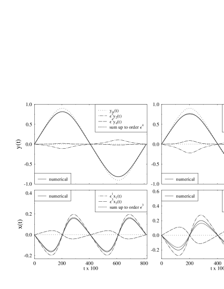
Figure 2: Coordinates $x(t)$ and $y(t)$ of the orbit R₅, evaluated at $\alpha=7$, ie $\epsilon=1$ (left side) and $\alpha=8$, ie $\epsilon=\sqrt{2}$ (right side). Solid lines: numerical results. Heavy dotted lines: perturbation series (9) including the terms in (24) up to 3rd and 4th order for $x(t)$ and $y(t)$, respectively. Other lines give partial contributions as labeled by the inserts. (Units such that $\hbar=1$; $E=1/6$.)

In figure 2 we compare the results obtained by summing the above analytical results according to (9) up to order $\epsilon^{4}$, shown by the heavy dotted lines, with the results obtained by numerical solution of the exact equations of motion (8), shown by the solid lines. The single contributions obtained at each order in $\epsilon$ are shown by the other lines, as labeled by the inserts. The left panels are calculated for $\alpha=7$ where $\epsilon=1$, and the right panels for $\alpha=8$ where $\epsilon=\sqrt{2}$. The convergence is surprisingly good even when the expansion parameter $\epsilon$ is larger than unity. This is due to the rapidly decreasing amplitudes of the $x_{k}(z)$ and $y_{k}(z)$ with increasing $k$. Note that for $y(t)$, where the agreement is perfect for $\epsilon=1$ and still very good for $\epsilon=\sqrt{2}$, we have included three terms, whereas $x(t)$ only contains two terms. Obtaining $x_{5}(z)$ would have required to calculate both $y_{6}(z)$ and $x_{7}(z)$ and to make them periodic, which – though analytically possible – would have been rather cumbersome. But the fact that the remaining errors in $x(t)$ are of the same order as $\epsilon^{4}y_{4}(z)$ suggests that adding the third term $\epsilon^{5}x_{5}(z)$ would lead to an equally good convergence for $x(t)$. Similar results were also obtained for other bifurcated orbits.

For the period-two orbits born at period-doubling bifurcations, the algebraic Lamé functions have to be used. The repeated integrations arising in the perturbation expansion then become more difficult and we could not do all of them analytically. Resorting to numerical integrations, however, whereby the coefficients $b_{k}$, $c_{k}$ and $d_{k}$ in (17) were determined numerically by iteration, we could reach a similar convergence of the perturbation series.

3 Semiclassical trace formulae for the density of states

In this section we shall apply our perturbative results to investigate the role of the pitchfork bifurcations of the A orbit in semiclassical calculations of the density of states. We coarse-grain both the exact and the semiclassical density of states by a convolution with a normalized Gaussian $\exp\{-(E/\gamma)^{2}\}/\gamma\sqrt{\pi}$. The quantum-mechanical coarse-grained density of states is then given by

$$g_{qm}(E)=\frac{1}{\gamma\sqrt{\pi}}\sum_{n}\exp\{-[(E-E_{n})/\gamma]^{2}\}$$ (25)

in terms of the exact quantum spectrum $\{E_{n}\}$ which we have obtained by diagonalization of (1) in a harmonic oscillator basis. For larger values of $\gamma$, the prominent gross-shell structure in the density of states is emphasized while finer details of its oscillations are suppressed. In the limit $\gamma\to 0$ the sum of delta functions is recovered. The oscillating part of (25) is defined as

$$\delta g_{qm}(E)=g_{qm}(E)-g_{TF}(E)\,,$$ (26)

where $g_{TF}(E)$ is the average part obtained in the Thomas-Fermi approximation which for the Q4 potential can be calculated analytically:

$$g_{TF}(E) = \frac{2}{\pi\hbar^{2}}\,K\!\left(\!\sqrt{(1-\alpha)/2}\,\right)\!\sqrt{E}\hskip 102.43008pt\hbox{for }-1<\alpha\leq+1\,,$$ (27)

$$= \frac{2}{\pi\hbar^{2}}\,\sqrt{\frac{2}{\alpha+1}}\,K\!\left(\!\sqrt{(\alpha-1)/(\alpha+1)}\,\right)\!\sqrt{E}\qquad\quad\hbox{for }\;\alpha\geq+1\,.$$

Higher-order $\hbar$ corrections to the average density of states [18] are negligible in the present system.

The semiclassical trace formula for the density of states has the general form

$$\delta g_{sc}(E)=\frac{1}{\pi\hbar}\sum_{po}{\cal A}_{po}(E)\,f_{\gamma}(T_{po})\,\cos\left[\frac{1}{\hbar}\,S_{po}(E)-\sigma_{po}\frac{\pi}{2}\right].$$ (28)

The sum goes over all periodic orbits ($po$) of the classical system. $S_{po}(E)$ are the action integrals $\oint{\bf p}\cdot d{\bf q}$ along the periodic orbits and $\sigma_{po}$ the so-called Maslov indices. The amplitudes ${\cal A}_{po}(E)$ depend on the number of constants of motion of the system. The factor $f_{\gamma}(T_{po})$ is given by [18]

$$f_{\gamma}(T_{po})=\exp\left[{-(\gamma\,T_{po}/2\hbar)^{2}}\right],$$ (29)

where $T_{po}=dS_{po}(E)/dE$ are the periods of the orbits. This coarse-graining factor favours the contributions of the shortest orbits to the gross-shell structure obtained with larger values of $\gamma$. When the system possesses no other constant of the motion besides the energy, all orbits are isolated and Gutzwiller’s original form [17] of the amplitudes ${\cal A}_{po}(E)$ applies. In the presence of continuous symmetries, and for integrable systems in general, other forms must be used (see [18] for a survey of trace formulae and the calculation of ${\cal A}_{po}$ and $\sigma_{po}$).

In the presence of bifurcations, the Gutzwiller amplitudes ${\cal A}_{po}(E)$ for isolated orbits cannot be used. However, the uniform approximation for generic pitchfork bifurcations [19, 20] can be applied to describe the isochronous bifurcations of the A orbit discussed in this paper. The factor 2 appearing in the period doubling for the generic case here plays the role of the extra degeneracy factor 2 of the bifurcated orbit pairs, which is due either to their reflection symmetry at the symmetry axis containing the A orbit (for the librating orbits L_n) or to the time reversal symmetry (for the rotating orbits R_n). Adapting the results of [20] to the present system, the combined contribution to the semiclassical density of states from all the orbits participating in the bifurcation at $\alpha_{n}$ (including their degeneracy factors) is given by

$$\delta g_{sc}^{bif}(E,\alpha_{n})=\frac{T_{\rm A}\,\Gamma(1/4)}{\pi\sqrt{2\pi}\,\hbar^{5/4}|a_{n}|^{1/4}k^{3/4}}\,\cos\left[\frac{kS_{\rm A}}{\hbar}-k\nu_{n}\frac{\pi}{2}-(-1)^{n}\frac{\pi}{4}-{\rm sign}(a_{n})\frac{\pi}{8}\right].$$ (30)

Here $k$ is the repetition number of the orbits and $\nu_{n}$ the Maslov index, corresponding to $\sigma_{po}$ in (28), of the unstable primitive orbit involved. The parameter $a_{n}$ stems from the normal form of the action function $S(q^{\prime},p)$ used in the phase-space representation of the trace integral at the $n$-th bifurcation of the A orbit. From the expansions given in [20] for the properties of the periodic orbits near the bifurcation, and using our results in the previous section, we can determine $a_{n}$ to be

$$a_{n}=\frac{1}{4S_{\rm A}}\left(\frac{4\pi}{2n+1}\right)^{2}\frac{1}{\tau_{4}(n)}\,.$$ (31)

In the following, we want to examine the importance of the contribution (30) in relation to that of other non-bifurcating orbits of the system. Quite generally, in an integrable two-dimensional system the leading families of degenerate orbits have an amplitude proportional to $\hbar^{-3/2}$ (except, eg, for harmonic oscillators with rational frequency ratios, where the leading amplitudes go like $\hbar^{-2}$, see [21]). They are therefore expected to dominate over the bifurcating orbits which here have an amplitude proportional to $\hbar^{-5/4}$ as seen in (30). In section 3.1 below we will test the relative importance of the latter for the particular integrable situation given in our system for $\alpha=0$. On the other hand, the standard Gutzwiller amplitudes for isolated orbits in a non-integrable system go like $\hbar^{-1}$, so that the bifurcating orbits can be expected to play a larger relative role. As we will see in section 3.2 their relative weight is, however, subject to a rather subtle balance between the stability of the shortest isolated orbits and the $\alpha$ dependence of the factor $|a_{n}|^{-1/4}$ in the amplitude of (30).

3.1 The separable case $\alpha=0$

For $\alpha=0$ the potential (1) is separable and thus defines an integrable system in which the majority of the periodic orbits live on a 2D torus in phase space. The EBK quantization can therefore be applied to obtain a semiclassical quantum spectrum from which a trace formula is readily derived [22]. However, the system possesses also the isolated orbit A which undergoes a bifurcation at $\alpha=0$. As we see from figure 1 the orbit A, which is stable (A₃) for $0<\alpha<1$, becomes unstable (A₂) for $\alpha<0$; the orbit L₃ bifurcating from it exists only for $\alpha\leq 0$ and is stable for $-0.5\,\hbox{\kern 0.90005pt\lower 2.32501pt\hbox{$\sim$} \kern-10.07997pt\raise 2.32501pt\hbox{$<$} }\alpha<0$. This gives a nontrivial contribution to the density of states whose role will be investigated numerically below.

Straightforward EBK quantization of the 2D torus gives the approximate spectrum

$$E^{\rm EBK}_{n_{x}n_{y}}=(1/4)\,(6\pi\hbar/4\hbox{\bf K})^{4/3}\left[(n_{x}+1/2)^{4/3}+(n_{y}+1/2)^{4/3}\right].\qquad(n_{x},n_{y}=0,1,2,\dots)$$ (32)

From this we obtain in the standard way [22, 23] the following Berry-Tabor type trace formula to leading order in $\hbar$:

$$\delta g_{sc}^{2D}(E)=\left(\frac{4\hbox{\bf K}}{2\pi\hbar}\right)^{\!3/2}\!(4E)^{1/8}\;2\!\!\!\sum_{n,m=1}^{\infty}(-1)^{n+m}\,\frac{nm}{(n^{4}+m^{4})^{5/8}}\,f_{\gamma}(T_{nm})\,\cos\left[\frac{1}{\hbar}\,S_{nm}(E)-\frac{\pi}{4}\right].$$ (33)

The classical actions and periods

$$S_{nm}(E)=(4\hbox{\bf K}/3)\,(4E)^{3/4}\,(n^{4}+m^{4})^{1/4},\qquad T_{nm}(E)=4\hbox{\bf K}\,(4E)^{-1/4}\,(n^{4}+m^{4})^{1/4}$$ (34)

of the 2D rational tori ($n,m$) correspond to the periodic orbits

$$x(t)=w_{x}\,{\rm cn}(w_{x}t+\phi)\,,\qquad y(t)=w_{y}\,{\rm cn}(w_{y}t)\,,\quad\;\,$$ (35)

with

$$w_{x}=(4E)^{1/4}\,n\,(n^{4}+m^{4})^{-1/4},\qquad w_{y}=(4E)^{1/4}\,m\,(n^{4}+m^{4})^{-1/4}.$$ (36)

These orbits form degenerate families described by the parameter $\phi\in[0,4\hbox{\bf K})$. The $(n,n)$ resonances are the families containing the $n$-th repetitions of the orbits B (for $\phi=0$ or $2\hbox{\bf K}$) and C (for $\phi=\hbox{\bf K}$ or $3\hbox{\bf K}$). Summation over all resonances $(n,m)$ with $n,m>0$ yields the trace formula (33).

However, the system also contains the isolated resonances $(n,0)$ and ($0,m$) with $n,m=1,2,3,\dots$ which correspond to the (repeated) one-dimensional A orbits in the $x$ and $y$ direction. With the uniform approximation (30) discussed above, we can include them in the trace formula, together with the orbits L₃ born at the bifurcation A${}_{3}\to$ A₂ + L₃. This gives the following common contribution of all A and L orbits and their $k$-th repetitions

$$\delta g_{sc}^{\rm AL}(E)=\frac{(4\hbox{\bf K})^{3/4}}{(\pi\hbar)^{5/4}}\,(4E)^{-1/16}\sum_{k=1}^{\infty}(-1)^{k}\frac{1}{k^{3/4}}\,f_{\gamma}(kT_{\rm A})\,\cos\left[\frac{k}{\hbar}S_{\rm A}(E)-\frac{3\pi}{8}\right]\!,$$ (37)

where $S_{\rm A}(E)=(4\hbox{\bf K}/3)\,(4E)^{3/4}$ is the action of the primitive A orbit. Hereby we have used the value $\tau_{4}=3\pi^{2}\!/16\hbox{\bf K}^{4}$ for the L₃ orbit as given in table 2, and the relation [9] $\Gamma(1/4)=(4\sqrt{\pi}\,\hbox{\bf K})^{1/2}$.

The total oscillating part of the semiclassical density of states at $\alpha=0$ then is given by the sum of the contributions (33) and (37). We observe that the latter is of order $\hbar^{1/4}$ relative to the leading-order contributions of the 2D torus families. (For isolated orbits, this relative factor would be $\hbar^{1/2}$ as mentioned above.) We therefore expect that the bifurcating orbits have a non-negligible influence on the density of states, at least for low energies where the negative power of $E$ in the amplitude of (37) does not suppress their contribution too much.

In figure 3 we show the coarse-grained level densities obtained with $\gamma=1$ (in units such that $\hbar=1$); the periodic orbit sums in (33) and (37) can here be limited to $n_{max}=m_{max}=k_{max}=2$. In the upper panel, we show separately the semiclassical results (33) of the 2D tori (solid line) and (37) of the bifurcating orbits (dotted line). Both are seen to have a monotonously increasing amplitude of the oscillations, whereas the quantum result (dashed line) exhibits a pronounced beating structure. When adding both semiclassical contributions, as shown in the lower panel, the quantum result is nicely reproduced. The quantum beat is clearly the result of the interference between the shortest orbits of the torus family on one hand and the bifurcating isolated orbits A and L₃ on the other hand.

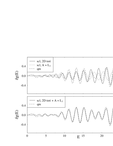
Figure 3: Oscillating part of the coarse-grained density of states at $\alpha=0$ (units such that $\hbar=1$; Gaussian smoothing width $\gamma=1$). Dashed lines: quantum-mechanical results (26). Solid and dotted lines: semiclassical results with $n_{max}=m_{max}=k_{max}=2$. Upper panel: separate contributions (33) of 2D tori and (37) of bifurcating orbits A + L₃. Lower panel: the solid line is here the sum of both semiclassical contributions.

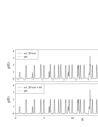
Figure 4: The same as figure 3, but for the total densities of states including the average part (27), with $\gamma=0.06$. Periodic orbit sums are cut at $n_{max}=m_{max}=k_{max}=30$.

The effect of the bifurcating orbits is less dramatic when we choose a finer resolution of the energy spectrum, obtained with a smaller value of $\gamma$. In figure 4 we show the total density of state including the average part (27), obtained for $\gamma=0.06$. Hereby periodic orbits up to $n_{max}=m_{max}=k_{max}\simeq 30$ contribute to the semiclassical results. We have normalized $g\,(E)$ here by the factor $\gamma\sqrt{\pi}$ so that the quantum result exhibits the correct degeneracies 1 or 2. Some apparently wrong higher degeneracies are badly resolved accidental (near-)degeneracies. At first glance there is not much of a difference between the upper and lower panels of figure 4. However, a closer inspection reveals that the semiclassical degeneracies are wrong, with errors of up to $\sim 20\%$, in the upper part where only the 2D tori are included. They come much closer to the exact ones when including the bifurcating orbits, as seen in the lower panel. There also the bottom regions between the peaks are improved, the remaining small oscillations being numerical noise. Note that the inclusion of the bifurcating orbits does not affect the semiclassical peak positions which are exactly those of the spectrum $E_{nm}^{\rm EBK}$ given in (32). The shifts in the peaks seen at the lowest energies are due to the typical errors inherent in the EBK approximation, which rapidly decrease with increasing energy.

3.2 The non-integrable case $\alpha=6$

As an example of a non-integrable situation we choose $\alpha=6$ where the rotating orbit R₅ is born at the bifurcation A${}_{5}\to$ A₆ + R₅. In figure 5 we show a Poincaré surface of section $(y,p_{y})$ taken at $x=0$. The large regular island in the middle contains the orbits A and R₅ at the origin. At its border we see an island chain of eight pairs of stable and unstable orbits born from a period-quadrupling bifurcation of the A orbit at $\alpha=5.4306$; the scaling properties of these fixed points were investigated in [6]. The four drop-like small regular islands around $(y,p_{y})=(\pm 0.431,\pm 0.362)$ contain the stable librating orbits S₃ that are born from the B orbits in the isochronous pitchfork bifurcation B${}_{3}\to$ B₂ + S₃ at $\alpha=3$, as seen in figure 1. [This is the same scenario as A${}_{3}\to$ A₂ + L₃ at $\alpha=0$, obtained after the transformation $\alpha\to(3-\alpha)/(1+\alpha)$ discussed in the introduction.] The orbits S₃ are still stable at $\alpha=6$. Since their common periods and actions are smaller than those of the orbit A, we expect them to influence the gross-shell structure in the density of states.

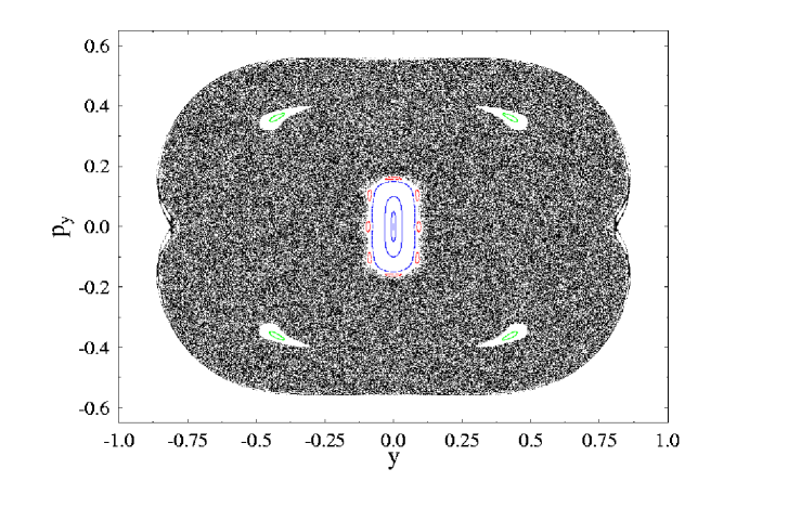
Figure 5: Poincaré surface of section (taken at $x=0$) for $\alpha=6$. See text for a discussion of the visible regular islands.

Clearly, there is no hope of obtaining full semiclassical quantization by summing over all periodic orbits in this mixed phase-space system, where many orbits of longer periods will also be close to bifurcations. However, we may try to obtain the coarse-grained density of states using only the shortest periodic orbits, as in figure 3 above, and thus using a cut-off $k_{max}$ of the sum over the repetition number $k$. The contribution of the four S₃ orbits to the semiclassical trace formula has the standard form for a stable isolated orbit [17, 24]:

$$\delta g_{sc}^{S_{3}}(E)=\frac{2}{\pi\hbar}\,T_{{\rm S}_{3}}(E)\sum_{k=1}^{k_{max}}\frac{(-1)^{k}}{\sin(k\chi_{{\rm S}_{3}}/2)}\,f_{\gamma}(kT_{{\rm S}_{3}})\sin\left[\frac{k}{\hbar}\,S_{{\rm S}_{3}}(E)\right],$$ (38)

whereby the period $T_{{\rm S}_{3}}(E)$, the action integral $S_{{\rm S}_{3}}(E)$ and the stability angle $\chi_{{\rm S}_{3}}$ have been determined numerically. The contribution from the bifurcating A and R orbits is given by (30) with $\nu_{n}=6$ and using (31) with $\tau_{4}=-11/1260$ according to table 2 for $n=3$.

Figure 6 shows the coarse-grained density of states obtained with a Gaussian smoothing width of $\gamma=1.0$, including only the $k_{max}=2$ lowest harmonics of the shortest periodic orbits. The upper panel gives the separate contributions of the isolated S₃ orbits (solid line) and of the bifurcating A and R orbits (dotted line); the lower panel gives their sum. The dashed lines give the quantum-mechanical result in both panels. As in the case shown in figure 3, each of the single contributions give a monotonically increasing amplitude of the oscillations in $\delta g_{sc}(E)$, and only their superposition yields a beating result that reproduces the quantum-mechanical result fairly well. The remaining discrepancies must be due to the missing contributions from other orbits with longer periods, of which there are already many at $\alpha=6$.

In spite of the fact that their amplitude in (30) is larger by a relative factor $\hbar^{-1/4}$ than that of the isolated orbits, the overall contribution of the bifurcating orbits to the coarse-grained density of states is seen in the upper part of figure 6 to be lower. This has two reasons. First, the shortest isolated orbits $S_{3}$ have a period that is substantially smaller than that of the orbits A and R₅, which leads to a larger value of the coarse-graining factor $f_{\gamma}$ in the trace formula. Second, the orbits $S_{3}$ are stable and have therefore a stability denominator of order unity, whereas the amplitude in (30) has a larger overall denominator. Still, the uniform A + R₅ contribution is strong enough to cause the beating interference pattern seen in the total $\delta g_{sc}(E)$.

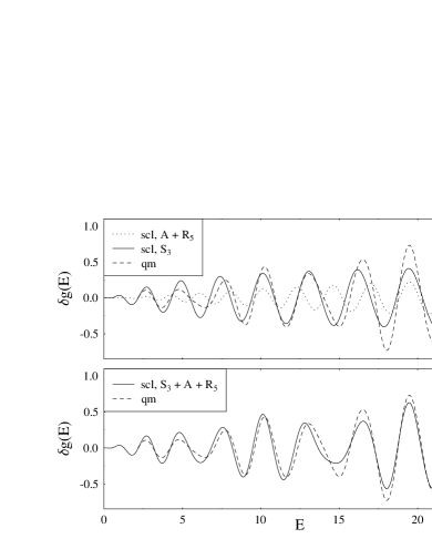
Figure 6: Oscillating part of density of states as in figure 3, but at $\alpha=6$. Upper panel: separate contributions of the stable isolated orbit S₃ (solid line) and of the bifurcating orbits A + R₅ (dotted line). Lower panel: sum of orbits S₃ + A + R₅ (solid line). Truncation of the trace formulae (30) and (38) at $k_{max}=2$, Gaussian averaging width $\gamma=1.0$. The dashed line in both panels gives the quantum-mechanical result.

It is now interesting to speculate about the relative contribution of the bifurcating orbits when the parameter $\alpha$ is further increased on the route towards chaos. On one hand, the average stability of the shortest isolated orbits can be expected to decrease. On the other hand, figure 7 reveals that the uniform amplitude in (30) of the period-one ($k=1$) orbit A with its offsprings at the bifurcation

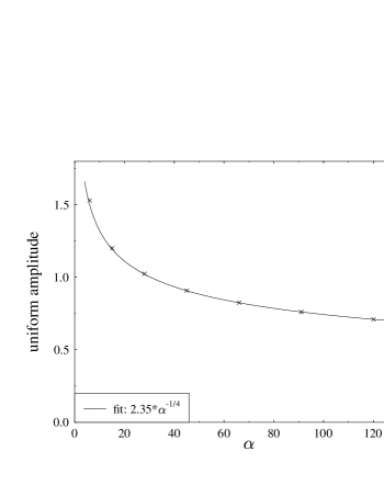
Figure 7: Amplitude of the uniform approximation (30) for the bifurcating A orbit ($k=1$) to the semiclassical density of states ($E=1/6$). The crosses give the values obtained using the values of $\tau_{4}$ in table 2 for $n>0$ at the bifurcation points $\alpha_{n}$; the solid line is an asymptotic fit for large $\alpha$.

points also decreases with increasing $\alpha_{n}$. (The crosses give the analytical values obtained using the $\tau_{4}$ values from table 2, and the solid line is a numerical fit showing that the amplitude decays asymptotically like $\alpha^{-1/4}$.) Taking furthermore account of the fact that more and more new pairs of isolated orbits are created from the bifurcations along the route to chaos (and new orbits bifurcate from these again), even the number of shortest (period-one) isolated orbits increases very fast. We therefore tend to conclude that the relative weight of the bifurcating orbits in the coarse-grained density of states will decrease with $\alpha$. It would, however, require a major numerical effort to study this balance in more detail and, in particular, to investigate the contributions from higher repetitions to the finer details of the density of states.

4 Summary

We have formulated a perturbative scheme to calculate analytically the shapes of periodic orbits bifurcating from the straight-line orbits in the quartic oscillator potential, exploiting the nice properties of the periodic Lamé functions in terms of Jacobi elliptic functions. In order to simplify the recursive determination of the unknown constants in the perturbation expansion, we have used an unconventional a posteriori rescaling of the perturbed solutions that takes care of the varying periods of the bifurcated orbits.

For stable period-one orbits we are able to give analytical expressions of the resulting perturbative series. Even when the perturbation parameter $\epsilon$ is greater than unity, satisfactory convergence to the numerically obtained solutions can be reached by going up to order $\epsilon^{4}$ where the necessary algebraic work is still not too demanding.

We have studied semiclassical trace formulae for approximating the quantum-mechanical density of states of the quartic oscillator. In the separable case $\alpha=0$ we could give a completely analytical trace formula, consisting of the contributions (27), (33) and (37). It was shown numerically to give a very good approximation to the exact quantum-mechanical density of states. Its low-frequency part, extracted with an energy coarse-graining parameter $\gamma=1$, reveals a strong quantum beat. This beat can only be reproduced semiclassically when the shortest periodic orbit families are allowed to interfere with the isolated orbits A and L₃ taking part in a pitchfork bifurcation. The contribution of the latter was calculated using a slightly modified uniform approximation for generic pitchfork bifurcations given in (37). The high-resolution spectrum is dominated by the Berry-Tabor part (33) which yields exactly the peaks corresponding to the EBK spectrum. The quantum degeneracies are, however, substantially affected by the contributions from the bifurcating orbits.

In the non-integrable situation $\alpha=6$, which exhibits a strongly mixed phase space, we could also reproduce the coarse-grained quantum density of states semiclassically, including besides the bifurcating period-one orbits A and R₅ also the shortest stable isolated orbits S₃ which had to be obtained numerically. The two types of orbits interfere, again leading to a beat structure. Finally, we have shown the uniform contribution of the bifurcating A orbits and its offsprings to decrease like $\alpha^{-1/4}$ for further increasing values of the chaoticity parameter $\alpha$.

With these results we have demonstrated the possibility of accessing analytically the periodic orbits in a system with mixed classical dynamics. We hope to stimulate further research in this direction, in particular towards semiclassical studies of the role of periodic orbits and their bifurcations in connection with spectral statistics [2, 25], which would have exceeded the scope of our present short report. We also aim at further improving our understanding of the uniformization of semiclassical trace formulae, including bifurcations of higher codimensions and – as a long-term (and perhaps too ambitious?) goal – including complete bifurcation cascades.

Note added in proof

We have confirmed the result (37) in an alternative way, without making use of any normal form. We start from the Poisson summation-integration of the density of states $\sum_{n_{x},n_{y}}\delta(E-E_{n_{x},n_{y}}^{EBK})$ using the EBK spectrum (32), like in the standard derivation [22] of (33). The first integration can be done exactly exploiting the delta function. For the edge contributions corresponding to the A and L₃ orbits, the usual stationary phase approximation cannot be used and the second integration must be done more carefully. Its asymptotic evaluation, valid here for $kS_{\rm A}/\hbar\,\hbox{\kern 0.90005pt\lower 2.32501pt\hbox{$\sim$} \kern-10.07997pt\raise 2.32501pt\hbox{$>$} }2$, leads precisely to the analytical result (37).

Acknowledgements

We are grateful to Jörg Kaidel for helpful discussions and Christian Amann for providing us with a program for the numerical computation of the quantum spectrum. SNF, AGM and MM acknowledge the hospitality of the University of Regensburg during their research visits and financial support by the Deutsche Forschungsgemeinschaft.

References

- [1]
-
[2]
Zimmermann Th, Meyer H-D, Köppel H and Cederbaum L S
1986 Phys. Rev. A 33 4334
Meyer H-D 1986 J. Chem. Phys. 84 3147 -
[3]
Eckardt B 1988 Phys. Rep. 163 205
Eckardt B, Hose G and Pollak E 1989 Phys. Rev. A 39 3776 - [4] Bohigas O, Tomsovic S and Ullmo U 1993 Phys. Rep. 223 43
- [5] Eriksson A B and Dahlqvist P 1993 Phys. Rev. E 47 1002
- [6] Lakhshminarayan A, Santhanam M S and Sheorey V B 1996 Phys. Rev. Lett. 76 396
- [7] Dahlqvist P and Russberg G 1990 Phys. Rev. Lett. 65 2837
- [8] Brack M, Mehta M and Tanaka K 2001 J. Phys. A 34 8199
- [9] Gradshteyn I S and Ryzhik I M 1994 Table of Integrals, Series, and Products (Academic Press, New York, 5th edition) ch 8.1
- [10] Erdélyi A et al 1955 Higher Transcendental Functions vol 3 (New York: McGraw-Hill) ch 15
- [11] Yoshida H 1984 Celest. Mech. 32 73
- [12] Ince E L 1940 Proc. R. Soc. 60 47
- [13] Ince E L 1940 Proc. R. Soc. 60 83
- [14] Erdélyi A 1941 Phil. Mag. 32 348
-
[15]
Brack M 2001 Foundations of Physics vol 31,
ed A Inomata et al p 209
(Festschrift in honor of the 75th birthday
of Martin Gutzwiller)
(Brack M 2000 LANL preprint nlin.CD/0006034) - [16] Whittacker E T and Watson G N 1969 A course of modern analysis 4th edn (Cambridge: University Press)
- [17] Gutzwiller M C 1971 J. Math. Phys. 12 343
- [18] Brack M and Bhaduri R K 1997 Semiclassical Physics Frontiers in Physics vol 96 (Reading, MA: Addison-Wesley) Revised paperback edition to appear in January 2003 (Boulder, CO: Westview Press)
- [19] Ozorio de Almeida A M and Hannay J H 1987 J. Phys. A 20 5873
- [20] Schomerus H and Sieber M 1997 J. Phys. A 30 4537, and earlier references quoted therein
- [21] Brack M and Jain S R 1995 Phys. Rev. A 51, 3462
- [22] Berry M V and Tabor M 1976 Proc. R. Soc. 349, 101
- [23] Creagh S C and Littlejohn R G 1992 J. Phys. A 25, 1643
- [24] Miller W H 1975 J. Chem. Phys. 63 996
-
[25]
Bogomolny E B and Keating J P 1996 Phys. Rev. Lett.
77 1472
Berry M V, Keating J P and Prado S D 1998 J. Phys. A 31 L245
Sieber M and Richter K 2001 Physica Scripta T 90 128