Stationary and moving breathers in a simplified model of curved alpha–helix proteins

Abstract

The existence, stability and movability of breathers in a model for alpha-helix proteins is studied. This model basically consists a chain of dipole moments parallel to it. The existence of localized linear modes brings about that the system has a characteristic frequency, which depends on the curvature of the chain. Hard breathers are stable, while soft ones experiment subharmonic instabilities that preserve, however the localization. Moving breathers can travel across the bending point for small curvature and are reflected when it is increased. No trapping of breathers takes place.

1 Introduction

In the last years quite a great deal of research is being done on localization due to the interplay of nonlinearity and geometry, either with the Nonlinear Schrödinger Equation [1, 2], FPU models [3, 4, 5], Klein–Gordon models [6, 7] or in DNA models [8, 9]. The objective is to understand the role of the bending points in biomolecules: whether localized excitations can travel across them or not and whether there are points where energy is stored and play a biological function. The description of the biological systems is given by variables, that represent internal or external degrees of freedom, which oscillate with time and are coupled by different potentials. A change of geometry can be felt by the system by different physical mechanisms, modelled correspondingly: interaction between nearest and next neighbours [4, 5]; potentials that depend on the angles [1] or long–range interaction due to the dipole–dipole coupling [2, 6, 7].

Simplifying, the effect of a curved chain can be described easily. For stationary excitations the zone where the chain of oscillators is bent is inhomogeneous, bringing about the existence of localized linear modes which compete strongly with the nonlinear localized modes. For high coupling the linear localization predominates, for low coupling the nonlinear localization is the important one. The transition from one regime to the other can be continuous or discontinuous as the parameters are changed or the curvature increases [7]. Moving excitations, have to travel across this inhomogeneous zone. The excitation within the bending zone needs a different energy, which can be larger than in the straight system, therefore acting as a barrier. The excitation can be reflected, transmitted or trapped [10].

The alpha–helix protein is another molecule for which is interesting to investigate the role of the bending in the existence, shape, properties and transport of localized excitations. The peptide groups have a dipole moment parallel to the chain and the Amide-I excitations interact among them through acoustic phonons. The dipole-dipole interaction to be described in detail below makes the system sensitive to the shape of the molecule. Apart from the interest of the biophysical problem in itself, it has a relevant feature from a more theoretical point of view: it is only necessary to take into account the nearest neighbours in order that the system can feel the bending of the chain. To our knowledge the effect of the curvature in such a system with dipoles parallel to the chain have not yet been described.

There are different excitations that can be considered, as solitons, envelope solitons and discrete breathers. Here we focus our research on the latter. As it is well known, discrete breathers are very localized oscillations that appear as a consequence of nonlinearity and discreteness [11, 12, 13, 14]. They are, therefore, specially relevant in biomolecules when considering excitations that involve only a few units, far from the continuous limits. Although a relatively new field, stationary breathers are now well understood and research is presently focusing on the possible physical and biological consequences of their existence and in future technological applications, specially with Josephson-junctions [15, 16]. Moving breathers is not such a mature field: there are techniques to obtain them but many questions remain unanswered [17, 18]. Perhaps the most important one is the reason why they exist in some systems and not in others. New developments are given in [19].

This study intends to complete previous works [6, 7, 10] on the properties of localization and transmission of energy in bent chains, described by Klein–Gordon models. The models in the references cited are inspired in DNA, with three main properties:

1. There is long–range interaction between dipole moments.

2. The dipoles moments are perpendicular to the chain and to the plane of curvature.

3. The effect of the curvature enters the model as a shortening of the distances between dipole moments.

The simplified alpha–helix model studied here, apart from its different physical origin, has the following differences:

1. The only interactions considered are nearest–neighbour. Note that the DNA models cited, without long–range interaction would not feel at all the shape of the molecule.

2. The dipole moments are parallel to chain and to the plane of curvature

3. The bending of the chain appear in the model as a change in the angles between dipole moments, and, therefore in the interaction energy.

In spite of these differences, both models present very similar behaviour both for predominant stronger attractive or repulsive interaction. This suggest that they are generic on bent Klein–Gordon systems.

However, this paper introduces a new point of view. Previous works misinterpreted the mathematical property of annihilation of breathers as the curvature is increased. What happens is that the bending forces the breather at the bending point to choose some frequency, which depends weakly on its energy.

This phenomenon, could be, in principle, tested experimentally. For example, the mean curvature of DNA depends on the solvents concentration, and the absorbtion of radiation by breathers at the bending points would appear at some characteristics frequencies, that change with the solvents concentration. The presence of some harmonics of these frequencies would differentiate breathers from linear localized modes. Certainly, many technical problems should be expected, but we are planning to perform this study with some experimental groups. Apparently, the more adequate molecule might be RNA due to its short persistence length.

The short section 6 deals with moving breathers. Its first objective is to check if in this model, breathers can move and are reflected by or transmitted through the bending point. The second is to confirm the trapping hypothesis introduced in Ref. [21] for a DNA model with an impurity. The role of an impurity is similar to a bending point in bringing about localized linear modes, which compete with the (nonlinear) breather localization. This hypothesis consist in the nonexistence of trapping for moving breathers when there exists a linear localized mode with different tail profile, i.e., neighbouring sites in phase or with opposite phase (and, therefore, different frequency). There exist no mathematical proof, but it is also confirmed in this work in spite of the differences stated above.

2 Model description

We describe the position of each amino acid by $\mathbf{r}_{n}$, $n$ being an index. The distance between amino acids is supposed to be a constant $a$, i.e. , $a=|\mathbf{r}_{n+1}-\mathbf{r}_{n}|$. The direction of the dipole moments are given by unit vectors $\mathbf{t}_{n}=\displaystyle\frac{(\mathbf{r}_{n+1}-\mathbf{r}_{n})}{|\mathbf{r}_{n+1}-\mathbf{r}_{n}|}$ and the moments themselves are given by $\mathbf{p}_{n}=p_{n}\,\mathbf{t}_{n}$.

The Hamiltonian of the system, for which details are given in  A, can be written as

$$H=\sum_{n}\ \displaystyle\frac{1}{2}{\dot{u}}^{2}_{n}+\displaystyle\frac{1}{2}\omega_{0}^{2}u_{n}^{2}+\Psi(u_{n})+\displaystyle\frac{1}{2}\varepsilon(u_{n+1}-u_{n})^{2}+\mu(\mathbf{t}_{n+1}-\mathbf{t}_{n})^{2}u_{n}u_{n+1}\,,$$ (1)

with $\omega_{0}=1$, and the on site potential is given by $V(u_{n})=\frac{1}{2}\omega_{0}^{2}u_{n}^{2}+\Psi(u_{n})$ , $\Psi(u_{n})$ being its nonlinear part.

The corresponding dynamical equations are

$${\ddot{u}}_{n}+\omega_{0}^{2}u_{n}+\Psi^{\prime}(u_{n})+\varepsilon(2\,u_{n}-u_{n+1}-u_{n-1})$$

$$\hbox to0.0pt{\hss${}+{}$}\;\mu((\mathbf{t}_{n+1}-\mathbf{t}_{n})^{2}u_{n+1}+(\mathbf{t}_{n-1}-\mathbf{t}_{n})^{2}u_{n-1})=0\,,$$ (2)

or, in a simplified notation

$$f_{n}(u)\equiv{\ddot{u}}_{n}+\omega_{0}^{2}u_{n}+\Psi^{\prime}(u_{n})+\varepsilon\sum_{m}C_{n,m}u_{m}+\mu\sum_{m}J_{n,m}u_{m}=0\,,\;$$ (3)

with the obvious definition of the coupling matrices $C$ and $J$. Note that $C$ does not depend on the parameters while $J$ depends only on the curvature $\kappa$

Certainly, many different shapes can be considered. Here we focus as in previous papers on a parabola in a two–dimensional space. The reason is that it is the simplest form to describe a bending point and it is an approximation of any curve in the neighbourhood of it. Other shapes considered in the literature like the hairpin geometry, although interesting in themselves are not so adequate for our purposes, because, for example, the latter is composed by three homogeneous regions (except if considering long–range interaction). Therefore, the vectors $\mathbf{r}_{n}$ have components $(x_{n},y_{n})$ with $y_{n}=\frac{1}{2}\kappa x_{n}^{2}$, $\kappa$ being the curvature.

A sketch of the model is shown if figure 1

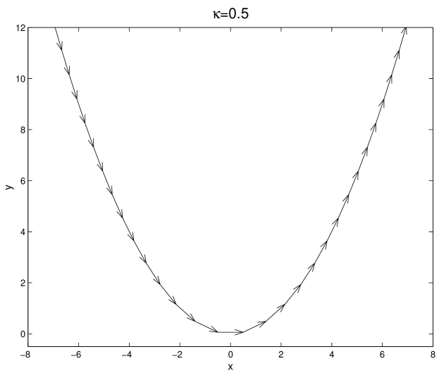
Figure 1: Sketch of the model for curvature $\kappa=0.5$.

In spite of having many dimensionless variables, there are still a few parameters in our problem: $\varepsilon$, which will be called the stacking coupling parameter, $\mu$, the dipole coupling parameter, the curvature $\kappa$ and the breather frequency, which we represent by $\omega_{\mathrm{b}}$. The distance of $\omega_{\mathrm{b}}$ from the phonon band is a measure of the degree of nonlinearity of the excitation. Generally speaking, the more nonlinear the excitation, the narrower it becomes. To explore thoroughly the parameter space is a daunting task but to obtain a general picture is a much more affordable one and this is what we intend here.

3 Linear modes

In bent systems there exist linear modes that are localized around the bending point. The first step is therefore to obtain the dependence of the linear spectrum on the parameters and identify the most important ones. The linear modes are the solutions of equation 3 with $\Psi=0$. We first obtain the dependence on the stacking parameter $\varepsilon$ without dipole coupling or equivalently for a straight chain, i.e., either $\mu=0$ or $(\mathbf{t}_{n+1}-\mathbf{t}_{n})=0,\;\forall n$ in Equation 3. Figure 2 shows this spectrum dependence.

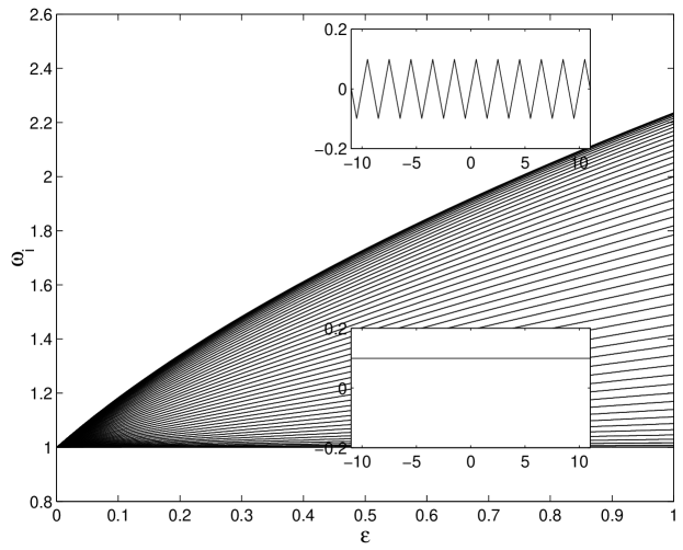
Figure 2: Dependence of the linear spectrum of the system on the stacking coupling parameter $\varepsilon$ for a straight chain. The insets show the shape of the linear modes with highest and lowest frequency.

This a well known spectrum, which we include here for comparison. Let us comment three facts: first, the spectrum is continuous; second, the mode with highest frequency consist of all oscillators vibrating with opposite phase with respect to the nearest neighbours; third, the mode with lowest frequency consist of all oscillators vibrating in phase. This modes will hereafter be denoted the top and the bottom mode, respectively.

When the stacking coupling $\varepsilon=0$ we have to choose either to represent the variation of the linear spectrum as a function of the parameter $\mu$ or to the curvature $\kappa$, the other parameters fixed at non–zero values. It turns out that both possibilities give similar results. Figure 3 shows the dependence of the linear spectrum on $\kappa$. There are three key features: first, there are localized modes that separate from the continuous spectrum; second, the top and bottom modes are localized within a radius of about a few units around the bending point and they become more localized as $\kappa$ increases; third, the top mode has all the oscillators in phase, which we will describe as being bell shaped, while the bottom mode has neighbouring oscillators with opposite phase (zig–zag shaped). This change of profile is due to a change of the predominant coupling interaction when $\kappa$ (or $\mu$) is increased. Around the bending point the sign in front of the variable $u_{m}$ in the coupling terms of equation (3) changes from negative, i.e, attractive interaction to positive, i.e., repulsive interaction. For homogeneous repulsive interaction the linear spectrum would be as in figure 2, but the frequencies spreading downwards and the zig–zag mode at the bottom.

The localization does not depend on the number of sites in the system. If the dipole coupling parameter $\mu$ is changed at constant curvature $\kappa$, the spectrum is very similar with a slightly larger spread of the frequencies except for the top and bottom modes.

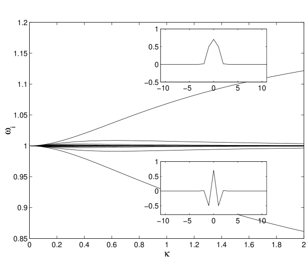
Figure 3: Dependence of the linear spectrum of the system on the curvature $\kappa$ with stacking coupling parameter $\varepsilon=0$ and dipole coupling parameter $\mu=0.2$. The insets show the bell and zig-zag shapes of the linear modes with highest and lowest frequency, respectively.

To conclude the description of the linear spectra we represent in figure 4 the dependence of the spectrum on the dipole parameter $\mu$ for a non–zero, constant value of the stacking parameter $\varepsilon=0.05$ and constant curvature $\kappa=1$. It can be seen that for some value of $\mu$ the same localized modes separate from the continuous spectrum. Note that while studying breathers these modes are going to be the ones competing with nonlinear excitations and be predominant for high enough coupling. The frequency $\omega_{\mathrm{b}}$ of the breathers have to be outside the continuous band or it will not be possible to obtain the breathers, which in physical terms means that the linear localized modes will resonate with the breather frequency and the energy will spread along the chain. If the on–site potential is hard, the breather frequency $\omega_{\mathrm{b}}$ will be above the phonon band, $\omega_{\mathrm{b}}>\omega_{0}$, therefore competing with the bell–shaped, top, linear mode. In the opposite case, $\omega_{\mathrm{b}}<\omega_{0}$, the competing mode will be the zig–zag shaped, bottom one. This will to be described in detail in the next section.

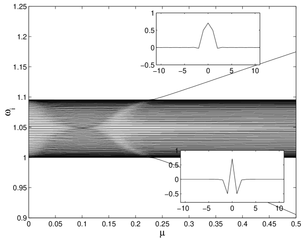
Figure 4: Dependence of the linear spectrum of the system on the dipole coupling parameter $\mu$ for constant stacking parameter $\varepsilon=0.05$ and curvature $\kappa=1$. The insets show the shape of the linear modes with highest and lowest frequency, respectively.

4 Hard breathers

To obtain breathers we need to choose the value of their frequency, which for a hard potential (here $V(u_{n})=\frac{1}{2}\omega_{0}^{2}u_{n}^{2}+1/4\,u_{n}^{4}$ ) will be above $\omega_{0}=1$. Let us choose $\omega_{\mathrm{b}}=1.2$, i.e., a frequency not too far from the phonon band but outside of it. The properties of the breathers with stacking coupling are well known, but we include them here for comparison. Figure 5 shows the profile of the breather while the parameter $\varepsilon$ is changed. The path continuation using the Newton method finishes as the phonon band expands and collides with the breather frequency. The breather profile is a zig-zag one, which can also be easily deduced by tail analysis.

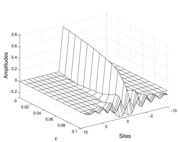
Figure 5: Dependence of the breather profile with hard, on–site potential for the straight chain on the stacking parameter $\varepsilon$. Frequency $\omega_{\mathrm{b}}=1.2$.

We obtain an analogous picture if the continuation is done with respect to the dipole coupling parameter $\mu$, for constant curvature, until a bifurcation point. Now the breather gets the bell profile shown in figure 6.

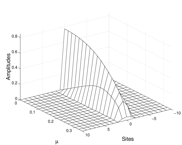
Figure 6: Dependence of the breather profile with hard on–site potential for a curved chain with curvature $\kappa=2$ on the dipole coupling parameter $\mu$ with constant frequency $\omega_{\mathrm{b}}=1.2$. $\varepsilon=0$

The fact that the breather amplitudes, i.e, $\{|u_{n}(0)|\}=\{\max_{\forall t}(|u_{n}(t)|)\}$, tend to zero is misleading. We are in presence of an annihilation bifurcation [20] , i.e., the Jacobian of the dynamical equation (3) with respect to $u=(u_{1},u_{2},\dots,u_{n})$ has an eigenvalue that tends to zero. This eigenvalue does not correspond to another breather in the neighbourhood of the parameter space but to the upper (for a hard potential) breather band [13] of the same breather. The physical meaning is that there are no localized excitation with the chosen frequency, except in the trivial case where the breather has zero amplitude, i.e., it is in the linear regime. We can obtain a complementary picture if the continuation is performed while keeping constant another characteristic of the breather. In [22] this is done with constant action, here, using a similar technique, we have chosen to keep the energy constant, which is physically meaningful.

By fixing the energy we restrict ourselves to the situation which is realized in single-molecule experiments. More biologically meaningful would be to keep constant not the energy but the temperature. This is however beyond the scope of our paper because to carry out this type of investigation it is necessary to introduce into equations of motion stochastic forces and solve corresponding Langevin equations.

The dependence of the breather profile on the parameter $\mu$ at constant energy is plotted in figure 7. It can be seen that allowing the breather the freedom of choosing its frequency the continuation is possible for much larger values of $\mu$, or, in physical terms, there exist localized breathers although not at any frequency. Note that in this situation the phonon band is very narrow, and what we have is a nonlinear version of the linear mode described previously, whose frequency is close to the breather’s one although not identical.

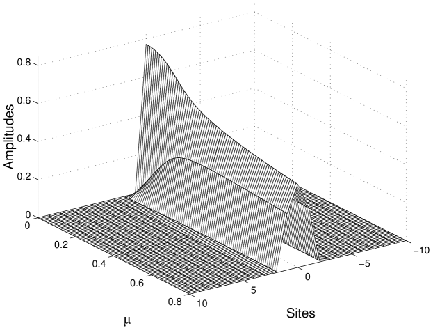
Figure 7: Dependence of the breather profile with hard on–site potential for a curved chain with curvature $\kappa=2$ on the dipole coupling parameter $\mu$ for constant energy, $E=0.3855$. The frequency changes from 1.2 to 1.46. $\varepsilon=0$.

Although the cases described above are interesting to understand the phenomena, the situation with more physical interest is the process of curving the chain. Suppose that $\varepsilon\neq 0$ and $\mu\neq 0$ and the breather has its frequency above the phonon band. When the chain is curved, the dependency of the breather with respect to the curvature is similar as with respect to $\mu$. If we choose to maintain constant the frequency the plot of the breather evolution is very similar to figure 6, except for the fact that at the zero curvature the breather would have a zig–zag profile which progressively changes to the bell profile for large enough curvature. Perhaps more interesting is choice of keeping the energy constant, as it is a conserved quantity. The dependence of the breather amplitudes and frequency are shown in figure 8. In the figure to the right we can see how the linear mode appears and the frequency of the top mode increases until almost colliding with the breather frequency. The breather with frequency $\omega_{\mathrm{b}}=1.2$ no longer exists while there exists a breather which is the nonlinear analogue of the top linear mode and its frequency increases as the chain is curved.

The linear mode is a solution of equation (3), with $\Psi=0$, or, equivalently, with almost zero amplitudes for $\Psi\neq 0$. What we have called its nonlinear analogue, is solution of the same equation with $\Psi\neq 0$ and has nonzero amplitudes, has a similar profile, as can it is shown in figure 8. It has more than a single harmonic in its linear spectrum. These extra harmonics are significatively larger for breathers with soft on–site potentials, as studied in the next section. In the case studied here, as the linear mode is localized, and, therefore, its frequency is isolated from the phonon band, the nonlinear analogue can be obtained by substituting $\Psi\rightarrow s\Psi$ in equation (3), and changing continuously $s$ from zero to $1$ at constant energy.

The observation of figure 8 shows that for frequencies above the top of the phonon band, i.e., slightly below $1.1$ for the parameters in the figure, it is only possible to continue the breather with the curvature at constant frequency until it approaches the top mode frequency curve. Thereafter, it is possible to continue it at constant energy, and its frequency follows slightly above the top mode.

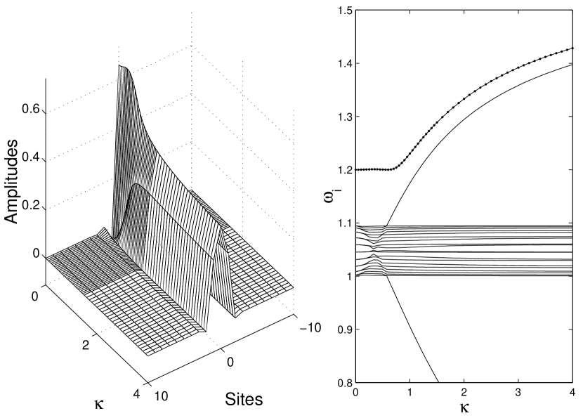
Figure 8: Left: Dependence of the breather profile with hard on–site potential for a curved chain on the curvature at constant energy. Right: Plot of the breather frequency (dots) and the linear spectrum with respect to the curvature. $E=0.3064$, $\varepsilon=0.05$, $\mu=0.5$.

If the chain is curved around the neighbouring site where the initial excitation is located, it will switch to the bending point, for even small curvature, when the frequency of the top linear mode approaches to its frequency. This happens at $\kappa=0.7$ for the values corresponding to figure 8. Similar behaviour has been found in reference [6].

Let us mention that all the breathers described here are linearly stable, i.e. all their Floquet eigenvalues have modulus $1$. The hard breathers in this system are always stable. The properties of the soft ones are very different.

5 Soft breathers

We have included the previous section for completeness, but, actually, in biological molecules, chemical bonds are thought to be better described by soft potentials. The most commonly used are the quartic soft, $V(u_{n})=\frac{1}{2}\omega_{0}^{2}u_{n}^{2}-\frac{1}{4}u_{n}^{4}$, the cubic potential, $V(u_{n})=\frac{1}{2}\omega_{0}^{2}u_{n}^{2}-\frac{1}{3}u_{n}^{3}$, the Lennard–Jones potential, $V(u_{n})=\sigma(1/r^{6}-1/r^{12})$, and the Morse potential $V(u_{n})=D(\exp(-b\,u_{n})-1)^{2}$. The last two are known to have several nice characteristics: a) they are asymmetric, with a hard part, that describes the strong repulsion when two atoms or molecules approach, and a soft part that becomes flat, reflecting the weakening of the bond when the molecules get separated and eventually unbonded; b) they have moving breathers with stacking coupling potentials; c) compared with another frequently used soft potential, the cubic one, it does not have an infinite well, which has no physical interpretation and can produce anomalous results when simulations are done. We have chosen for presenting our results the Morse potential because it is mathematically simpler, but the Lennard–Jones potential provides similar results.

For the straight chain and the normalized Morse potential $D=1/2$ and $b=1$, which gives the same frequency $\omega_{0}=1$ for small oscillations, and a representative frequency of the nonlinear excitations $\omega_{\mathrm{b}}=0.8$ , the breathers are bell-shaped, their amplitudes grow with the coupling parameter and they become unstable for $\varepsilon=0.12$. The nonlinear mode that produces the instability is an spatially asymmetric one. This will be of special interest in the section of moving breathers.

For stationary breathers, we are interested in values of the parameters where the dipole interaction is significant and the nonlinearity is weak. In this situation, typical parameters can be $\varepsilon=0.05$, $\mu=0.5$. For these parameters the frequencies of the phonon band, i.e., the continuous part of the linear spectrum, spread from $1$ to $1.1$. A rough measure of the nonlinearity of the excitation is the distance of its frequency from the phonon band, which suggest a frequency around $0.8$ or $0.9$.

If we start with the straight chain and a breather centered at the bending point and we increase the curvature at constant frequency, the same difficulties as with the hard breathers arise: the amplitudes of the breathers tend to zero when its frequency approaches the bottom linear mode and the continuation becomes impossible. We must emphasize this point: in the breather literature path continuation is usually done at constant frequency, which is a natural consequence of the theorems of existence [11] from the anticontinuous limit. At the anticontinuous limit there exists freedom to choose the frequency of the isolated oscillators and therefore at low coupling too. This is not the case if the system is in presence of strongly localized modes: there are no localized excitations at every frequency. This characteristic opens the possibility of spectroscopic analysis to check the existence of breathers in biomolecules and eventually to measure curvatures.

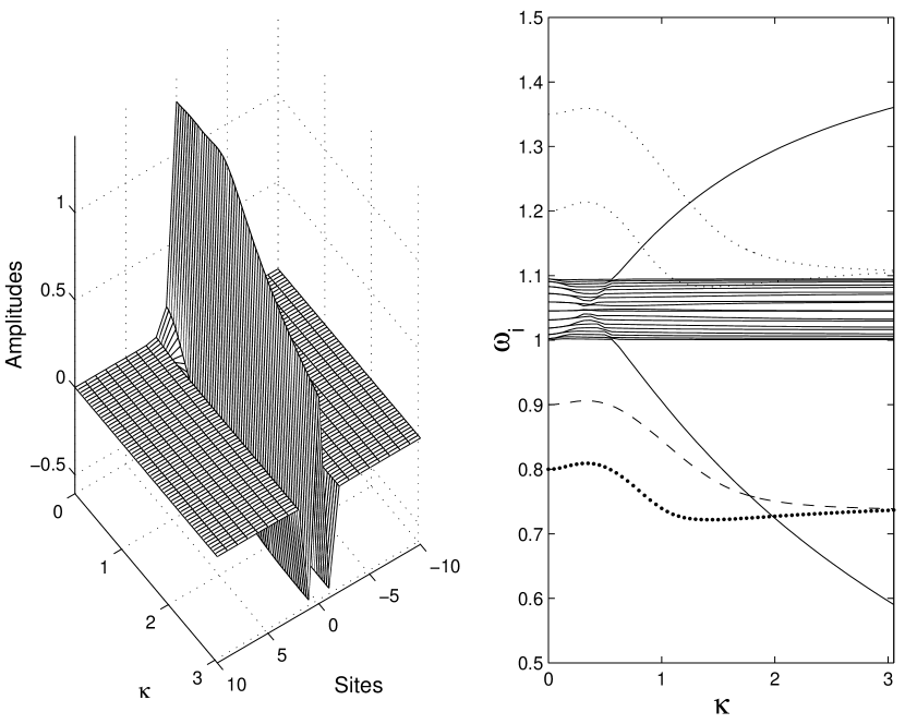
Figure 9: Left: Dependence of the breather profile with soft, on–site potential for a curved chain on the curvature at constant energy E=0.35. Right: Plot of the breather frequencies for two energies, E=0.35 (big dots) and E=0.20 (dashed), and 1.5 times the breather frequencies (small dots) and the linear spectrum (continuous lines) with respect to the curvature. Parameters: $\varepsilon=0.05$, $\mu=0.5$.

From the mathematical point of view, if the frequency is not fixed, we need to fix another quantity, and the chosen one, as previously, is the energy. Thus, the variation of the breather with the curvature mimics an adiabatic process of bending. Figure 9–left, shows the dependence of the breather profile with $\omega_{\mathrm{b}}=0.8$ at $\kappa=0$ on the curvature, changing its shape from a bell profile to a zig–zag one, until its becomes almost invariable. While this process takes place, its frequency changes, which is shown in figure 9–right. The breather becomes unstable at $\kappa\approx 0.8$. The frequencies of another breather with lower energy and higher frequency is also represented in this figure. The higher the frequency the larger becomes the curvature, for which instability is produced.

The exact stability analysis has been done calculating the Floquet eigenvalues, but we prefer to plot here the breather frequency, the linear spectrum and $1.5$ times the breather frequency. This gives a much more intuitive physical picture.

The reason for plotting this frequency is the following. When the curvature is increased, the frequencies $\{\omega_{i}\}$ of the internal modes, i.e., the small perturbation of the breather, are very similar to the ones shown in figure 4, as commented in section 3. The biggest difference is that the bottom mode (with soft on–site potential, and the top one for hard on–site potential) is not there, because this mode is substituted by the breather itself. The corresponding Floquet multipliers are $\{\lambda_{i}=\exp(\pm\,2\,\pi\,\omega_{i}/\omega_{\mathrm{b}})\}$, $\{\theta_{i}=\pm\,2\,\pi\,\omega_{i}/\omega_{\mathrm{b}}\}$ called the Floquet arguments. For a instability to be produced, a collision of two multipliers has two take place with the condition that they have the same Krein signature (See reference [13] for details on this subject). The positive (negative) Floquet arguments have all of them the same positive (negative) signature and cannot therefore bring about instabilities until they collide at ($1+0\,\mathrm{i}$), named harmonic instabilities, or ($-1+0\,\mathrm{i}$), subharmonic instabilities, or between them, named oscillatory instabilities or Krein crunches. The first one happens when $\theta_{i}=2\,\pi\,n$, $n\in\mathbb{N}$, for some $i$, that is, $\omega_{i}=n\,\omega_{\mathrm{b}}$, or in other words a linear mode resonates with the breather frequency or its harmonics. Figure 9 shows that this kind of bifurcation does not happen here.

The subharmonic instabilities can occur when $\theta_{i}=\pi+2\,n\,\pi$,, for some $i$, i.e., $\omega_{i}=\omega_{\mathrm{b}}/2+n\omega_{\mathrm{b}}$. Within the range of parameters studied, this can only occur when some $\omega_{i}$ equals $1.5\,\omega_{\mathrm{b}}$. Therefore, subharmonic instabilities appear in our system, when some frequency of the internal modes (very close to the linear ones, as commented above), collide with the $1.5\,\omega_{\mathrm{b}}$. This is easily seen plotting simultaneously the $1.5\,\omega_{\mathrm{b}}$ curve and the linear frequencies.

Figure 9–right shows the reason of this instability: the curve $1.5\,\omega_{\mathrm{b}}$ intersects with the frequency curve of the top linear mode, bringing about the instability. Nevertheless, the latter is a localized mode, centered at the bending point and the localization persists although the excitation has now superimposed a perturbation with twice the breather period. Within the range of parameters shown there are also a Krein crunches, related with perturbations of the frequency, but also preserving the localization. This happens after the Floquet multipliers of the phonon band have crossed at ($-1+0\mathrm{i}$), or, in other words, their frequency have become larger than $1.5\,\omega_{\mathrm{b}}$. The eigenvalues of the internal linear modes cross with other and do small excursions outside the unit circle. This is also evident, as the curve $1.5\,\omega_{\mathrm{b}}$ enters the phonon band. The same figure shows the frequency of a breather with higher energy corresponding to a frequency $\omega_{\mathrm{b}}=0.9$ at $\kappa=0$. Note that both breathers tend to the same frequency as the curvature increases and that breathers with energy slightly below $E=0.35$ avoid the secondary bifurcations, because the $1.5\,\omega_{\mathrm{b}}$ curve does not intersect the phonon band.

The apparent intersection of the breather frequency with the bottom linear mode is misleading because the latter does not exist as a perturbation of the breather, being this one its nonlinear analogue. The breather is not, however, linear, as its first AC harmonic is of the order of the DC one, and the second, about one third of it.

6 Moving breathers

In this section we explain briefly the behaviour of a moving breather in a curved region of the alpha–helix.

In order to move a breather, we apply the marginal mode method [17]. It basically consists in adding a spatially asymmetric mode (the pinning mode) to the breather velocity. As is shown in [20], the stacking coupling of the breather must be strong enough in order that it can be moved.

The scenario is similar to the observed in DNA chains [10] and biopolymers [4], i.e., for a fixed value of the curvature, there exists a critical value of the velocity below which the breather is reflected when it reaches the bending point and, above which, the breather crosses through it. Analogously, for a fixed value of the velocity, the breather crosses the bending point as long as the curvature is smaller than a critical value. As the curvature increases, the breather spends more and more time at the bending point and eventually is reflected. These two behaviours are shown in figures 10 and 11. In other words, the moving breather in a curved alpha–helix chain behaves as a particle in a potential barrier.

In reference [21] an hypothesis is introduced about the existence of trapping in inhomogeneous Klein–Gordon lattices. According to it, trapping of breathers does not occur when there exists a linear localized mode with a profile (vibration pattern or wave vector) different from the stationary breather one. When this occurs, the moving breather behaves as a particle in a potential barrier and is never trapped. As Figure 4 shows, there is a localized mode (the top mode) of opposite profile to the breather, and the case exposed in the reference cited above is the same as in the curved alpha–helix. The simulations confirm that the trapping hypothesis [21] holds in our system, and moving breathers cannot be trapped.

We still have not been able to find a counterexample, and this hypothesis seems generic for Klein–Gordon systems. However, it has no mathematical proof and should be checked as much as possible to achieve, at least, an inductive confirmation.

7 Conclusions

We have studied the existence and properties of stationary and moving breathers in a model with dipole moments parallel to a curved chain of oscillators. Its interest is twofold. On the one hand it is a model for a channel of amino acids along an alpha–helix protein, where the internal degrees of freedom are the Amida–I vibrations. In this aspect the objective of our work is to explore the role of the bendings as places where the energy is stored and to investigate whether moving excitations can travel across a bending point or not. On the other hand the theoretical interest comes from it being a model that completes previous works on bending chains. The specifics of the model are: a) the dipoles are oriented along the chain instead of perpendicular to it; b) it is sufficient to take in account nearest neighbours in order that the system can feel the shape of the chain.

In previous models [6, 7, 10, 20] the shape is felt due to the change between the distances of the oscillators, and, therefore, they need long–range interaction in inextensible chains. In our model the shape is felt due to the change of the angles between dipole moments. In this way, we expect to help to complete the study of systems in curved chains and approach to a generalized description.

The most important general fact, overlooked in the breather literature to our knowledge, is that the presence of strongly localized models around the bending point has such decisive a role: the breathers cannot be chosen at any frequency when the curvature is increased. Their interaction with the linear localized modes brings about frequencies approximately determined, and dependent on the curvature.

Consequently, we have developed a variant of the existing techniques, described in B to obtain breathers at constant energy. Therefore, the continuation of the breathers when the curvature is increased, models an adiabatic process of bending. More biologically meaningful would have been to model this process at constant temperature, but this is outside the scope of the techniques used in this paper, which are related more to single molecule experiments.

The adiabatic process of curving the chain transforms the initial breather into a nonlinear analogue to the top or bottom linear mode according to the on–site potential. The corresponding linear mode, therefore, do not exist in presence of the breather and cannot produce instabilities. The consequence is that hard breathers in the bent chain are stable and soft breathers experience subharmonic instabilities, that conserve, however, the localization.

We also have shown that up to curvatures relatively high, moving breathers can travel across the bending point spending some time at it. They cannot, however be, trapped, which confirms recent developments in the field [21].

The physical suggestion is that breathers may be a means of storage and transport of energy in proteins, due to and in spite of their complex structure in the space. Certainly, our model is a rough description of such complex a system, yet the main conclusion of the present and previous studies could be that the properties of breathers in different curved chains are quite common. We also think that they might provide a means to detect experimentally breathers at the bending points, showing absorbtion of characteristic frequencies and their harmonics, which depend on the curvature. We are, presently, in contact with experimental groups to explore its feasibility.

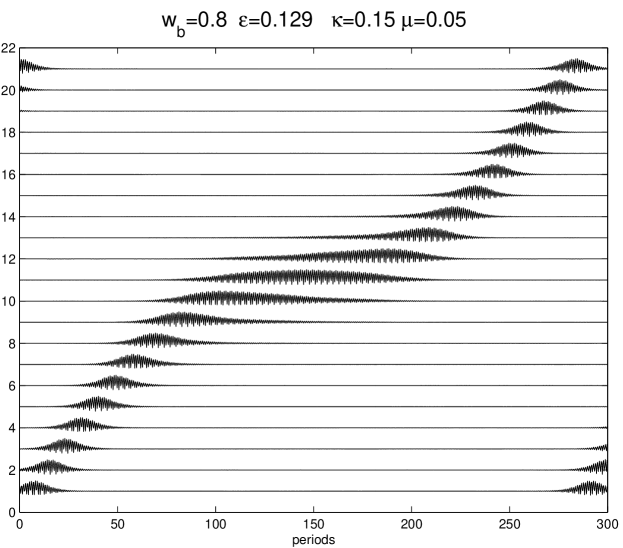
Figure 10: A breather travelling across the bending point. A small increase of the curvature will produce a reflection

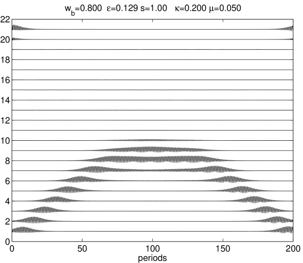
Figure 11: A breather being reflected at the bending point.

Appendix A Details of the model

As said in Section 1, we describe the position of each amino acid by a vector $\mathbf{r}_{n}$, $n$ being an index. The distance between amino acids is supposed to be a constant $a$, i.e. , $a=|\mathbf{r}_{n+1}-\mathbf{r}_{n}|$. The direction of the dipole moments are given by unit vectors $\mathbf{t}_{n}=(\mathbf{r}_{n+1}-\mathbf{r}_{n})/|\mathbf{r}_{n+1}-\mathbf{r}_{n}|$ and the moments themselves are given by $\mathbf{p}_{n}=p_{n}\,\mathbf{t}_{n}$.

The interaction energy between two neighbouring dipoles $n$ and $n+1$ is given by

$$\begin{array}[]{rl}U_{n,n+1}=&\displaystyle\frac{\mathbf{p}_{n+1}\mathbf{p}_{n}}{|\mathbf{r}_{n+1}-\mathbf{r}_{n}|^{3}}-3\displaystyle\frac{\mathbf{p}_{n}(\mathbf{r}_{n+1}-\mathbf{r}_{n})\cdot\mathbf{p}_{n+1}(\mathbf{r}_{n+1}-\mathbf{r}_{n})}{|\mathbf{r}_{n+1}-\mathbf{r}_{n}|^{5}}\\ =&p_{n+1}p_{n}\left(\displaystyle\frac{\mathbf{t}_{n}\mathbf{t}_{n+1}}{|\mathbf{r}_{n+1}-\mathbf{r}_{n}|^{3}}-3\displaystyle\frac{\mathbf{t}_{n}(\mathbf{r}_{n+1}-\mathbf{r}_{n})\cdot\mathbf{t}_{n+1}(\mathbf{r}_{n+1}-\mathbf{r}_{n})}{|\mathbf{r}_{n+1}-\mathbf{r}_{n}|^{5}}\right)\\ =&p_{n+1}p_{n}\left(\displaystyle\frac{\mathbf{t}_{n}\mathbf{t}_{n+1}}{a^{3}}-3a^{2}\displaystyle\frac{\mathbf{t}_{n}\mathbf{t}_{n}\cdot\mathbf{t}_{n+1}\mathbf{t}_{n}}{a^{5}}\right)\\ =&(p_{n+1}p_{n}/a^{3})\left(-2\mathbf{t}_{n+1}\mathbf{t}_{n}\right)=(p_{n+1}p_{n}/a^{3})\left((\mathbf{t}_{n+1}-\mathbf{t}_{n})^{2}-2\right)\mbox{}\end{array}$$ (4)

Suppose that the equilibrium value of $p_{n}=p_{0},\;\forall n$, then we can express its non equilibrium value as $p_{n}=p_{0}+q\,u_{n}$, where $u_{n}$ represent the stretching from the equilibrium positions. Substitution into Equation 4 leads to

$$U_{n,n+1}=U^{0}_{n,n+1}+U^{1}_{n,n+1}+\left(-2\displaystyle\frac{q^{2}}{a^{3}}+\displaystyle\frac{q^{2}}{a^{3}}(\mathbf{t}_{n+1}-\mathbf{t}_{n})^{2}\right)u_{n+1}u_{n}\;\;$$ (5)

The first two terms in this equation stand for constant and linear terms, therefore, they will not appear in the Hamiltonian, as its first derivatives with respect to the variables $u_{n}$ at equilibrium, i.e., $u_{n}=0$ must be zero. We represent the remaining term by $H_{n,n+1}$.

Suppose that the Hamiltonian of the system is given by

$$H=\sum_{n}\displaystyle\frac{1}{2}{\dot{u}}^{2}_{n}+\displaystyle\frac{1}{2}\alpha^{2}u_{n}^{2}+\Psi(u_{n})+\displaystyle\frac{1}{2}K(u_{n+1}-u_{n})^{2}+H_{n,n+1}\;,\;$$ (6)

where $\alpha$ and $K$ are positive constants and $\Psi(u_{n})$ is the nonlinear part of the on–site potential. Rearranging the terms we obtain

$$H=\sum_{n}\ \displaystyle\frac{1}{2}{\dot{u}}^{2}_{n}+\displaystyle\frac{1}{2}(\alpha^{2}-4\displaystyle\frac{q^{2}}{a^{3}})u_{n}^{2}+\Psi(u_{n})\mbox{}$$

$$\hbox to0.0pt{\hss${}+{}$}\,\displaystyle\frac{1}{2}(K+2\displaystyle\frac{q^{2}}{a^{3}})(u_{n+1}-u_{n})^{2}+\displaystyle\frac{q^{2}}{a^{3}}(\mathbf{t}_{n+1}-\mathbf{t}_{n})^{2}u_{n+1}u_{n}$$ (7)

Thus, the Hamiltonian can be written as

$$H=\sum_{n}\ \displaystyle\frac{1}{2}{\dot{u}}^{2}_{n}+\displaystyle\frac{1}{2}\omega_{0}^{2}u_{n}^{2}+\Psi(u_{n})+\displaystyle\frac{1}{2}\varepsilon(u_{n+1}-u_{n})^{2}+\mu(\mathbf{t}_{n+1}-\mathbf{t}_{n})^{2}u_{n+1}u_{n}\;,$$

with $\omega_{0}=1$, $\varepsilon=(K+2\,q^{2}/a^{3})/\alpha^{\prime 2}$, $\mu=q^{2}/(a^{3}\alpha^{\prime 2})$, where $\alpha^{\prime 2}=\alpha^{2}-4\,q^{2}/a^{3}$, with the time rescaled $t\rightarrow\alpha^{\prime}t$ and the redefinition of $\Psi(u_{n})\rightarrow\Psi(u_{n})/\alpha^{\prime 2}$. The initial Hamiltonian has been also divided by $\alpha^{\prime 2}$,

We keep the term $w_{0}$ in the formulae in spite of being $1$ as a reference because its meaning is the frequency at very low amplitude when the oscillators are isolated.

The corresponding dynamical equations are

$${\ddot{u}}_{n}+\omega_{0}^{2}u_{n}+\Psi^{\prime}(u_{n})+\varepsilon(2\,u_{n}-u_{n+1}-u_{n})$$

$$\hbox to0.0pt{\hss${}+{}$}\,\mu((\mathbf{t}_{n+1}-\mathbf{t}_{n})^{2}u_{n+1}+(\mathbf{t}_{n-1}-\mathbf{t}_{n})^{2}u_{n-1})=0,$$ (8)

which are written in a simplified notation in Equation 3.

Appendix B Breathers with constant energy

To obtain breathers with constant energy, we use a variant of the method in the time-Fourier space [12, 23]. First, we obtain breathers by path continuation at constant frequency from the anticontinuous limit using the Newton method as described in the references above. Thereafter, the path continuation is performed at constant energy. In this case our variant applies and we give below the details needed to obtain the corresponding Jacobian used by the Newton method. It is also a variant of the method developed in [22] at constant action.

The Hamiltonian of the system can be written:

$$H=\displaystyle\frac{1}{2}\sum_{n}\dot{u}_{n}^{2}+W(u,\kappa)\,,$$ (9)

where $u=(u_{1},\dots,u_{N})$, and $W(u,\kappa)$ represents the potential energy, sum of the on–site and coupling energies; $\kappa$ represents any parameter, as the curvature in this article. The dynamical equations are given by $\ddot{u}_{n}+\displaystyle\frac{\partial W}{\partial u_{n}}=0$. Time-reversible periodic solutions with frequency $\omega_{\mathrm{b}}$ are given by a truncated Fourier series:

$$u_{n}(t)=\sum_{k=0}^{k_{m}}(2-\delta_{k,0})\,z_{k,n}\cos(k\,\omega_{\mathrm{b}}t)$$ (10)

The use of functions with different frequencies is inconvenient and can be avoided by the change of variable $\tilde{t}=\omega_{\mathrm{b}}t$, which leads to the Hamiltonian:

$$H=\displaystyle\frac{1}{2}\omega_{\mathrm{b}}^{2}\sum_{n}u_{n}^{\prime 2}+W(u,\kappa),$$ (11)

where $\prime{}$ represent the derivative with respect to $\tilde{t}$. The corresponding dynamical equations are:

$$f_{n}(u,\omega_{\mathrm{b}},\kappa)\equiv\omega_{\mathrm{b}}^{2}u_{n}^{\prime\prime}+\displaystyle\frac{\partial W}{\partial u_{n}}=0$$ (12)

In this equations $\omega_{\mathrm{b}}$ enters as a parameter and the functions $u_{n}$, with frequency unity in the new time variable, are given by:

$$u_{n}(\tilde{t})=\sum_{k=0}^{k_{m}}(2-\delta_{k,0})z_{k,n}\cos(k\tilde{t})$$ (13)

Therefore, the functions $f_{n}$ can be seen as $2\pi$-periodic functions of $\tilde{t}$ due to their dependence on $u(\tilde{t})$ and $u^{\prime\prime}(\tilde{t})$.

The components of the cosine discrete Fourier transform of the dynamical equations (12) are given by:

$$F_{k}[f_{n}]=-k^{2}\omega_{\mathrm{b}}^{2}z_{k,n}+F_{k}[\displaystyle\frac{\partial W}{\partial u_{n}}(u(\tilde{t}))]\,,$$ (14)

where $F_{k}[g(\tilde{t})]$ represent the k-th term in the cosine discrete Fourier transform of a $2\pi$ periodic function $g(\tilde{t})$, given by:

$$F_{k}[g(\tilde{t})]=\displaystyle\frac{1}{2\,k_{m}+1}\sum_{m=0}^{k_{m}}(2-\delta_{m,0})\,g(\displaystyle\frac{2\pi m}{2\,k_{m}+1})\,\cos(\displaystyle\frac{2\pi k\,m}{2\,k_{m}+1})$$ (15)

In this way, finding a breather is reduced to solve the $(k_{m}+1)\times N$ equations (14). As a breather solution is determined by the same number of Fourier coefficients $z_{k,n}$ and the frequency $\omega_{\mathrm{b}}$, we need and extra equation. If we are interested in obtaining solutions with given energy $E$, this is given by $H-E=0$, which for time-reversible solutions ($u_{n}^{\prime}(0)=0$) reduces to

$$F_{H}\equiv W(u(0),\kappa)-E=0$$

We denote by $\tilde{z}$ and $\tilde{F}$ the column matrices $(\{z_{k,n}\},\omega_{\mathrm{b}})$ and $(\{F_{k}[f_{n}]\},F_{H})$, respectively, with the index $k$ running faster. In order to use the Newton method for path continuation with the parameter $\kappa$ we need the Jacobian:

$$\frac{\partial\tilde{F}}{\partial\tilde{z}}=\left[\begin{array}[]{ccc}\Bigg{[}\left\{\displaystyle\frac{\partial F_{k}[f_{n}]}{\partial z_{k^{\prime},n^{\prime}}}\right\}\Bigg{]}&\begin{array}[]{c}\displaystyle\frac{\partial F_{k}[f_{n}]}{\partial\omega_{\mathrm{b}}}\\ \vdots\end{array}\\ \begin{array}[]{cc}\left\{\displaystyle\frac{\partial F_{H}}{\partial z_{k^{\prime},n^{\prime}}}\right\}&\dots\end{array}&\displaystyle\frac{\partial F_{H}}{\partial\omega_{\mathrm{b}}}\end{array}\right]$$ (16)

The left upper block is the Jacobian at constant frequency, its elements given by:

$$\frac{\partial F_{k}[f_{n}]}{\partial z_{k^{\prime},n^{\prime}}}=-k^{2}\omega_{\mathrm{b}}^{2}\delta_{k,k^{\prime}}\delta_{n,n^{\prime}}+\displaystyle\frac{2-\delta_{0,k^{\prime}}}{2}\left(F_{k+k^{\prime}}[\displaystyle\frac{\partial^{2}W}{\partial u_{n}\partial u_{n^{\prime}}}]+F_{|k-k^{\prime}|}[\displaystyle\frac{\partial^{2}W}{\partial u_{n}\partial u_{n^{\prime}}}]\right)$$ (17)

The elements in the last column are given by:

$$\frac{\partial F_{k}[f_{n}]}{\partial\omega_{\mathrm{b}}}=-k^{2}\omega_{\mathrm{b}}z_{k,n}\quad;\quad\displaystyle\frac{\partial F_{H}}{\partial\omega_{\mathrm{b}}}=\displaystyle\frac{\partial W(u(0))}{\partial\omega_{\mathrm{b}}}=0$$ (18)

The remaining elements in the last row are:

$$\displaystyle\frac{\partial F_{H}}{\partial z_{k^{\prime},n^{\prime}}}=\displaystyle\frac{\partial W(\{u_{n}(0)\})}{\partial z_{k^{\prime},n^{\prime}}}=\displaystyle\frac{\partial W(\{\sum_{l=0}^{k_{m}}(2-\delta_{l,0})z_{l,m}\})}{\partial z_{k^{\prime},n^{\prime}}}\,=\,\left(\displaystyle\frac{\partial W}{\partial u_{n^{\prime}}}\right)_{t=0}(2-\delta_{k^{\prime},0})\,$$

$$\hbox to0.0pt{\hss${}={}$}\,-\ddot{u}_{n^{\prime}}(0)\,(2-\delta_{k^{\prime},0})\,\,=\,(\sum_{l=0}^{k_{m}}l^{2}\omega_{\mathrm{b}}^{2}z_{l,n^{\prime}})\,(2-\delta_{k^{\prime},0})$$ (19)

References

References

- [1] YB Gaididei, SF Mingaleev, and PL Christiansen. Curvature–induced symmetry breaking in nolinear Schrödinger models. Phys. Rev. E., 62(1):R53–R56, 2000.
- [2] PL Christiansen, YuB Gaididei, and SF Mingaleev. Effects of finite curvature on soliton dynamics in a chain of nonlinear oscillators. J. Phys. Condens. Matter, 13(6):1181–1192, 2001.
- [3] R Reigada, JM Sancho, M Ibañes, and GP Tsironis. Resonant motion of discrete breathers in curved nonlinear chains. J. Phys. A, 34(41):8465–75, 2001.
- [4] M Ibañes, JM Sancho, and GP Tsironis. Dynamical properties of discrete breathers in curved chains with first and second neighbors interaction. Phys. Rev. E, 65:041902–041914, 2002.
- [5] GP Tsironis, M Ibañes, and JM Sancho. Transport of localized vibrational energy in biopolymer models with rigidity. Europhys. Lett., 57:697–703, 2002.
- [6] JFR Archilla, PL Christiansen SF Mingaleev, and Yu B Gaididei. Numerical study of breathers in a bent chain of oscillators with long range interaction. J. Phys. A, 34(33):6363–6373, 2001.
- [7] JFR Archilla, PL Christiansen, and Yu B Gaididei. Interplay of nonlinearity and geometry in a DNA–related, Klein-Gordon model with long–range dipole–dipole interaction. Phys. Rev. E, 65(1):016609–016616, 2001.
- [8] JJL Ting and M Peyrard. Effective breather trapping mechanism for DNA transcription. Phys. Rev. E, 53(1B):1011–20, 1996.
- [9] K. Forinash, T. Cretegny, and M. Peyrard. Local modes and localization in a multicomponent nonlinear lattice. Phys. Rev. E, 55(4):4740–4756, 1997.
- [10] J Cuevas, F Palmero, JFR Archilla, and FR Romero. Moving breathers in a bent DNA-related model. Phys. Lett. A, 299(2–3):221–225, 2002.
- [11] RS MacKay and S Aubry. Proof of existence of breathers for time-reversible or Hamiltonian networks of weakly coupled oscillators. Nonlinearity, 7:1623–1643, 1994.
- [12] JL Marín and S Aubry. Breathers in nonlinear lattices: Numerical calculation from the anticontinuous limit. Nonlinearity, 9:1501–1528, 1996.
- [13] S Aubry. Breathers in nonlinear lattices: Existence, linear stability and quantization. Physica D, 103:201–250, 1997.
- [14] S Flach and CR Willis. Discrete breathers. Physics Reports, 295:181–264, 1998.
- [15] P Binder, D Abraimov, and AV Ustinov. Diversity of discrete breathers observed in a Josephson ladder. Phys. Rev. E, 62(2):2858–62, 2000.
- [16] E Trias, JJ Mazo, and TP Orlando. Discrete breathers in nonlinear lattices: Experimental detection in a Josephson array. Phys. Rev. Lett., 84:741–744, 2000.
- [17] S. Aubry Ding Chen and George Tsironis. Breather mobility in discrete nonlinear lattices. Phys. Rev. Lett., 77:4776–4779, 1996.
- [18] S Aubry and T Cretegny. Mobility and reactivity of discrete breathers. Physica D, 119:34–46, 1998.
- [19] RS Mackay and JA Sepulchre. Effective Hamiltonian for travelling discrete breathers. J. Phys. A, 2002. To appear.
- [20] J Cuevas, JFR Archilla, Yu B Gaididei, and FR Romero. Moving breathers in a DNA model with competing short and long range dispersive interactions. Physica D, 163:106–126, 2002.
- [21] J Cuevas, F Palmero, JFR Archilla, and FR Romero. Moving discrete breathers in a Klein–Gordon chain with an impurity. Submitted, 2002.
- [22] JFR Archilla, RS MacKay, and JL Marín. Discrete breathers and Anderson modes: two faces of the same phenomenon? Physica D, 134:406–418, 1999.
- [23] JL Marín. Intrinsic Localised Modes in Nonlinear Lattices. PhD dissertation, University of Zaragoza, Department of Condensed Matter, June 1997.