We argue that the integrable modified nonlinear Schrödinger equation with the nonlinearity dispersion term is the true starting point to analytically describe subpicosecond pulse dynamics in monomode fibers. Contrary to the known assertions, solitons of this equation are free of self-steepening and the breather formation is possible.

1. Introduction

Soliton-based optical communication systems serve as an exciting example of the application of a purely mathematical concept (soliton) to modern technology. The nonlinear Schrödinger equation (NSE)

$$iu_{t}+(1/2)u_{xx}+|u|^{2}u=0$$ (1)

is the adequate model to describe picosecond soliton evolution in monomode fibers [1]. Here $u(x,t)$ is the envelope of the pulse electric field and coordinates $t$ and $x$ measure distance along the fiber and time in a frame comoving with the pulse group velocity, respectively. The applicability of NSE depends crucially on the assumption that the spatial width of the envelope is much larger that the carrier wavelength. Besides, the success of this model is substantially related to integrability of NSE [2] and hence to the controllability of soliton parameters [3]. Various more subtle effects accompanying the picosecond soliton propagation are usually treated as a perturbation of the integrable model.

On the other hand, dynamics of subpicosecond optical pulses ($\leq 100$ fs) is not well governed by NSE because the above mentioned assumption is not satisfied. The spectral width of subpicosecond pulses becomes comparable with the carrier frequency, and three main additional effects - nonlinearity dispersion, intrapulse Raman stimulated scattering and linear higher-order dispersion - should be taken into account [4]:

$$iu_{t}+(1/2)u_{xx}+|u|^{2}u=i\alpha_{1}\left(|u|^{2}u\right)_{x}+\alpha_{2}\left(|u|^{2}\right)_{x}u+i\alpha_{3}u_{xxx}.$$ (2)

The terms in rhs of (2) account for the above additional effects. In general, extra terms violate integrability of the equation. Hence, a question can be posed: does there exist an equation that will be integrable as NSE and at the same time would be more relevant in the subpicosecond range? The answer is positive because the modified NSE (MNSE)

$$iu_{t}+(1/2)u_{xx}+|u|^{2}u+i\alpha\left(|u|^{2}u\right)_{x}=0,\quad\alpha\in\rm{Re}$$ (3)

with the $\alpha$-dependent nonlinearity dispersion term is still integrable though the associated spectral problem is more involved than the Zakharov-Shabat one. Namely, the initial-value problem for MNSE (3) can be solved within the framework of the Wadati-Konno-Ichikawa (WKI) spectral problem [5]. A careful study of the WKI spectral problem (or the quadratic bundle) for MNSE and related equations was undertaken by Gerdjikov and Ivanov [6]. Explicit soliton solutions to MNSE obtained in [7] and [8] turned out too complicated for practical use. That is the reason that MNSE is usually treated as NSE with $\alpha$-dependent perturbation term, especially as actual values of $\alpha$ are normally small.

Among the other things, such treatment gave rise to some misunderstanding. First, it was shown in [9] that the initially symmetric hyperbolic-secant pulse evolving in accordance with MNSE (3) develops an asymmetric self-phase modulation and a self-steepening. There is a wide-spread opinion that the self-steepening is an inherent property of the subpicosecond pulse dynamics [4] that should be minimized for proper operation of an information system. Second, it is well known [10] that the initial pulse $2\,{\rm{sech}}\,x$ evolving according to NSE produces the NSE breather (the bound state of two solitons). On the other hand, the same initial pulse decays into separate solitons when evolving according to MNSE. Hence, it was inferred that MNSE does not admit breathers (or higher-order solitons) [11].

Our aim here is to show that the situation with subpicosecond soliton dynamics is rather different. We argue that the integrable MNSE is the true starting point to analytically describe this dynamics. It is remarkable that numerical simulations of the MNSE-based soliton propagation revealed various regimes which cannot be explained by treating the $\alpha$-dependent term in (3) as a perturbation of NSE [12]. We derive the MNSE soliton solution that is non-perturbative w.r.t. $\alpha$ and demonstrate that the MNSE soliton propagates without any self-steepening. Besides, we explicitly obtain breather solution to MNSE. Numerical simulations confirm the stability of the MNSE breather.

2. MNSE soliton

We will employ the Riemann-Hilbert (RH) problem [13] for solving nonlinear equations. Let us start with the Lax pair for MNSE (3):

$$\Psi_{x}=\Lambda(k)\left[\sigma_{3},\Psi\right]+2ikQ\Psi,\quad$$ (4)

$$\Psi_{t}=\Omega(k)\left[\sigma_{3},\Psi\right]+\biggl{(}\frac{4i}{\alpha}k^{3}Q+2ik^{2}Q^{2}\sigma_{3}-\frac{i}{\alpha}kQ+kQ_{x}\sigma_{3}-2i\alpha kQ^{3}\biggr{)}\Psi,$$

$$\Lambda(k)=-\frac{2i}{\alpha}\left(k^{2}-\frac{1}{4}\right),\quad\Omega(k)=-\frac{4i}{\alpha^{2}}\left(k^{2}-\frac{1}{4}\right)^{2}.$$

Here the Hermitian matrix $Q=\pmatrix{0&u\cr\bar{u}&0\cr}$ stands for the potential of the spectral problem (4), $k$ is a spectral parameter. The standard procedure is:
a) building the Jost solutions of the linear spectral problem (4);
b) building the solutions $\Phi_{\pm}$ which are analytical in complementary regions of the $k$-plane;
c) formulation of the RH problem for $\Phi_{\pm}$ with the standard normalization

$$\Phi_{\pm}\rightarrow I\qquad{\rm for}\quad|k|\to\infty,$$ (5)

where $I$ is the identity matrix.

It is, however, easy to see by substituting the asymptotic expansion w.r.t. to $k^{-1}$ of $\Psi$ to the spectral problem (4) that this problem does not agree with the standard normalization. On the other hand, an associated equation with the fifth-order nonlinearity,

$$iv_{t}+(1/2)v_{xx}-i\alpha v^{2}\bar{v}_{x}+|v|^{2}v+\alpha^{2}|v|^{4}v=0$$ (6)

has the Lax pair as well with the WKI spectral problem

$$\Psi_{x}^{(A)} = \Lambda(k)[\sigma_{3},\Psi^{(A)}]+(2ikQ_{A}+i\alpha Q_{A}^{2}\sigma_{3})\Psi^{(A)},$$ (7)

$$Q_{A} = \pmatrix{0&v\cr\bar{v}&0\cr}$$

that agrees with the standard normalization, and with the same dispersion relation $\Omega(k)$ for the temporal Lax equation. Moreover, equations (3) and (6) are gauge equivalent and solutions of MNSE (3) follow from those of (6) by means of a simple algebraic relation

$$Q=g^{-1}Q_{A}g,\qquad g(x,t)=\Psi^{(A)}(k=0,x,t).$$ (8)

The associated equation (6) does not have such an obvious physical interpretation as the MNSE but it has an extremely simple soliton solution. Hence, we will not solve MNSE directly. Instead we will integrate the associated equation (6) and then will obtain solutions of MNSE by the algebraic relation (8).

We begin with the spectral problem (7) for the associated equation. At first we define the Jost solutions $J_{\pm}$, $J_{\pm}\rightarrow I$ at $x\to\pm\infty$, which are interrelated with the scattering matrix $S$, $J_{-}E=J_{+}ES$. Here $E=\exp\left(\Lambda(k)x\right)$. Dividing the Jost solutions into columns, $J_{\pm}=(J^{(1)}_{\pm},J^{(2)}_{\pm})$, it can be shown by the standard analysis of integral equations that the columns $J^{(1)}_{+}$ and $J^{(2)}_{-}$ are analytical in the first and third quadrants of the $k$-plane. Hence, the matrix function $\Phi_{+}=(J^{(1)}_{+},J^{(2)}_{-})$ is analytical as a whole in the same quadrants. The matrix $\Phi_{+}$ can be expressed in terms of the Jost solution $J_{+}$ and some entries of the scattering matrix:

$$\Phi_{+}=J_{+}ES_{+}E^{-1},\qquad S_{+}=\pmatrix{1&s_{12}\cr 0&s_{22}}.$$

Because the potential $Q_{A}$ is Hermitian, we have the involutions $\left[J_{\pm}(k)\right]^{\dagger}=\left[J_{\pm}(\bar{k})\right]^{-1}$, $S(k)^{\dagger}=S(k)^{-1}$. They allow us to introduce the matrix function $\Phi_{-}$, $\Phi_{-}^{-1}(k)=\Phi_{+}(\bar{k})^{\dagger}=ES_{+}^{\dagger}E^{-1}J_{+}^{-1}$ that is analytical in the second and forth quadrants. Thereby, we can pose the RH problem with the standard normalization,

$$\Phi_{-}^{-1}\Phi_{+}=EG(k)E^{-1},\qquad\Phi_{\pm}\rightarrow I\quad{\rm at}\quad k\to\infty,$$ (9)

where

$$G(k)=S_{+}^{\dagger}S_{+}=\pmatrix{1&s_{12}\cr{\bar{s}}_{12}&1},\quad k\!\in\!\!\left\{k=\xi-i\eta,\,\,\,\xi\eta=0\right\},$$

as a problem of analytical factorization of the non-degenerate matrix $G(k)$ defined on both the real and imaginary axes of the $k$-plane.

In general, the function $\Phi_{+}$ has zeros in some points $k_{j}$ lying in the first and third quadrants, $\det\Phi_{+}(k_{j})=0$. Hence, in these points there exist eigenvectors $|n_{j}\rangle$ with zero eigenvalue. It is important that zeros $k_{j}$ appear by pairs $(k_{j},-k_{j})$. It is a feature of the WKI spectral problem. Hence, the single soliton of the associated equation is determined by two zeros $k_{1}$ and $-k_{1}$. The zeros $k_{j}$, eigenvectors $|n_{j}\rangle$ and the matrix $G(k)$ comprise the RH data. Because we deal with the solitons only, $G(k)$ being related with the continuous spectrum of the spectral problem, is taken to be the identity matrix.

If $\Phi_{+}$ is a solution of the RH problem (9), it can be expanded in the asymptotic series $\Phi_{+}=I+\Phi^{(1)}_{+}/k+\Phi^{(2)}_{+}/k^{2}+\cdots$. Substituting this expansion into the spectral problem (7), we reconstruct the potential $Q_{A}$:

$$Q_{A}=(1/\alpha)[\sigma_{3},\,\Phi^{(1)}_{+}]=(2/\alpha)\sigma_{3}\Phi^{(1)}_{+}.$$ (10)

Now we derive a soliton of the associated equation (6). Let us have zeros $k_{1}$ and $-k_{1}$ and two eigenvectors $|n_{\pm}\rangle$. It can be easily shown that the eigenvectors obey the equations

$$|n_{+}\rangle_{x}=\Lambda(k_{1})\sigma_{3}|n_{+}\rangle,\qquad|n_{+}\rangle_{t}=\Omega(k_{1})\sigma_{3}|n_{+}\rangle.$$

Hence, we obtain explicit space and time dependencies of the eigenvectors,

$$|n_{+}\rangle = \left(\begin{array}[]{c}\exp[\Lambda(k_{1})x+\Omega(k_{1})t]\exp(a+i\phi_{0})\\ \exp[-\Lambda(k_{1})x-\Omega(k_{1})t]\end{array}\right),$$ (13)

$$|n_{-}\rangle = \sigma_{3}|n_{+}\rangle,\quad\langle n_{\pm}|=|n_{\pm}\rangle^{\dagger}.$$

Here $a,\phi_{0}={\rm const}$. It can be shown by the dressing method [13] that the matrix $\Phi_{+}$ is represented as ($k_{\pm}\equiv\pm k_{1}$)

$$\Phi_{+}(k)=I-\sum_{j,l=\pm}\frac{|n_{j}\rangle(D^{-1})_{j\,l}\langle n_{l}|}{k-\bar{k}_{l}},\qquad D_{j\,l}=\frac{\langle n_{j}\,|n_{l}\rangle}{k_{l}-\bar{k}_{j}},$$ (14)

$$\Phi_{-}^{-1}(k)=I+\sum_{j,l=\pm}\frac{|n_{j}\rangle(D^{-1})_{j\,l}\langle n_{l}|}{k-k_{j}}.$$

Because the eigenvectors are known explicitly, we can evaluate the matrix $\Phi_{+}$ as $\Phi_{+}(k)=I-D_{+}/(k-\bar{k}_{1})-D_{-}/(k+\bar{k}_{1})$, where

$$D_{+} = \frac{k_{1}^{2}-\bar{k}_{1}^{2}}{2}\left(\begin{array}[]{cc}e^{z}(k_{1}e^{-z}+{\bar{k}}_{1}e^{z})^{-1}&e^{i\varphi}(k_{1}e^{-z}+{\bar{k}}_{1}e^{z})^{-1}\\ e^{-i\varphi}(k_{1}e^{z}+{\bar{k}}_{1}e^{-z})^{-1}&e^{-z}(k_{1}e^{z}+{\bar{k}}_{1}e^{-z})^{-1}\end{array}\right),$$ (17)

$$D_{-} = -\sigma_{3}D_{+}\sigma_{3}.$$

We introduced here new independent variables $z$ and $\varphi$:

$$z=-(1/w)(x-Vt-x_{0}),\quad\varphi=Vx-(1/2)(V^{2}-w^{-2})t+\varphi_{0},$$

$$x_{0}=aw,\quad\varphi_{0}={\rm const},$$

where the soliton velocity $V$ and width $w$ (see below) are defined by

$$V=\frac{1}{2\alpha}\left(1-2(k_{1}^{2}+\bar{k}_{1}^{2})\right),\qquad w=\frac{1}{2i}\frac{\alpha}{k_{1}^{2}-\bar{k}_{1}^{2}}.$$

Hence, the eigenvalue $k_{1}$ is expressed in terms of velocity and width as

$$k_{1}=(1/2)(1-\alpha V-i\alpha/w)^{1/2},\qquad{\rm Im}k_{1}<0.$$ (18)

Expanding then $\Phi_{+}$ in the asymptotic series, we obtain from Eq. (10) the soliton solution of the associated equation:

$$v_{s}=\frac{i}{w}\frac{e^{i\varphi}}{k_{1}e^{-z}+{\bar{k}}_{1}e^{z}}.$$ (19)

It has indeed a very simple form.

An important aspect of the solution (13) should be noted. Namely, the parameter $\alpha$ that enters the soliton width $w$ appears in the denominator. Hence, we cannot reproduce the soliton (13) considering the associated equation (6) as the $\alpha$-perturbed NSE. Nevertheless, there exists a procedure [14] to perform the limit $\alpha\to 0$. Namely, representing $k_{1}$ as $k_{1}=(1/2)-(\alpha/2)\lambda_{1}+{\cal O}(\alpha^{2})$, we obtain in this limit from Eq. (13) the NSE soliton with the eigenvalue $\lambda_{1}$.

As regards the MNSE soliton $u_{s}$, it follows from $v_{s}$ by means of the algebraic relation (8). Indeed, $u_{s}=(g_{2}/g_{1})v_{s}$,

$$\left(\begin{array}[]{cc}g_{1}&0\\ 0&g_{2}\end{array}\right)=\Phi_{+}(k=0)=I+\frac{2}{\bar{k}_{1}}\left(\begin{array}[]{cc}D_{+11}&0\\ 0&D_{+22}\end{array}\right).$$

Explicitly we have

$$g_{1}=\frac{k_{1}}{\bar{k}_{1}}\frac{k_{1}e^{z}+\bar{k}_{1}e^{-z}}{k_{1}e^{-z}+\bar{k}_{1}e^{z}},\quad g_{2}=\frac{k_{1}}{\bar{k}_{1}}\frac{k_{1}e^{-z}+\bar{k}_{1}e^{z}}{k_{1}e^{z}+\bar{k}_{1}e^{-z}},$$

$$u_{s}=\frac{i}{w}\frac{k_{1}e^{-z}+{\bar{k}}_{1}e^{z}}{(k_{1}e^{z}+{\bar{k}}_{1}e^{-z})^{2}}e^{i\varphi}.$$ (20)

The MNSE soliton (14) looks much simpler than those derived in [7] and [8]. In the limit $\alpha\to 0$, the solitons of both the MNSE and the associated equation reproduce one and the same NSE soliton.

Square of module of $u_{s}$ (14) is written as

$$|u_{s}|^{2}=\frac{1}{w^{2}}(k_{1}e^{-z}+{\bar{k}}_{1}e^{z})^{-1}(k_{1}e^{z}+{\bar{k}}_{1}e^{-z})^{-1}$$

$$=\frac{1}{2w^{2}}\left[1-\alpha V+\sqrt{(1-\alpha V)^{2}+\frac{\alpha^{2}}{w^{2}}}\,{\rm cosh}\frac{2}{w}(x-Vt)\right]^{-1}.$$

We see from this relation that the envelope $|u_{s}|$ moves holding its shape, i.e., without any self-steepening.

3. MNSE breather

To derive the MNSE breather, we start from four zeros $\pm k_{1}$ and $\pm k_{2}$, where $k_{j}=(1/2)(1-\alpha V_{j}-i\alpha/w_{j})^{1/2},\quad{\rm Im}k_{j}<0$ (cf. Eq. (12)). Because we seek for a bound state of two solitons, we put $V_{1}=V_{2}\equiv V$ and, without loss of generality, $V=0$. We have four eigenvectors with the property $|n_{2j}\rangle=\sigma_{3}|n_{2j-1}\rangle$, $j=1,2$. Namely,

$$|n_{1}\rangle = \left(\begin{array}[]{c}\exp[-(x/2w_{1})+i(t/4w_{1}^{2})+i\varphi_{11}]\\ \exp[(x/2w_{1})-i(t/4w_{1}^{2})+i\varphi_{12}]\end{array}\right),$$ (23)

$$|n_{3}\rangle = \left(\begin{array}[]{c}\exp[-(x/2w_{2})+i(t/4w_{2}^{2})+i\varphi_{21}]\\ \exp[(x/2w_{2})-i(t/4w_{2}^{2})+i\varphi_{22}]\end{array}\right)$$ (26)

with a special relation for the constant phases $\varphi_{11}-\varphi_{12}-\varphi_{21}+\varphi_{22}=\pi$. Denote $\lambda_{2j-1}\equiv k_{j}$ and $\lambda_{2j}\equiv-k_{j}$, $j=1,2$. Then the matrix function $\Phi_{+}(k)$ for the breather is written as (cf. Eq. (11))

$$\Phi_{+}(k)=I-\sum_{m,n=1}^{4}\frac{|n_{m}\rangle(D^{-1})_{m\,n}\langle n_{n}|}{k-\bar{\lambda}_{n}},\quad D_{m\,n}=\frac{\langle n_{m}\,|n_{n}\rangle}{\lambda_{n}-\bar{\lambda}_{m}}.$$

We omit cumbersome but evident calculations performed along the lines of Sect. 2 and give below the explicit expression for the MNSE breather at rest:

$$u_{br} = (g_{2}^{\prime}/g_{1}^{\prime})v_{br},$$ (27)

$$v_{br} = \frac{w_{1}-w_{2}}{w_{1}+w_{2}}D^{-1}\Bigl{[}w_{1}\left(k_{1}e^{x/w_{1}}+\bar{k}_{1}e^{-x/w_{1}}\right)e^{it/2w_{2}^{2}}$$

$$+ w_{2}\left(k_{2}e^{x/w_{2}}+\bar{k}_{2}e^{-x/w_{2}}\right)e^{it/2w_{2}^{2}}\Bigr{]},$$

$$D = w_{1}w_{2}\left(k_{1}e^{x/w_{1}}+\bar{k}_{1}e^{-x/w_{1}}\right)\left(k_{2}e^{x/w_{2}}+\bar{k}_{2}e^{-x/w_{2}}\right)$$

$$- w_{+}^{2}\left(k_{1}e^{x/w_{+}-it/w_{+}w_{-}}-\bar{k}_{2}e^{-x/w_{+}+it/w_{+}w_{-}}\right)$$

$$\times \left(k_{2}e^{x/w_{+}+it/w_{+}w_{-}}-\bar{k}_{1}e^{-x/w_{+}-it/w_{+}w_{-}}\right),$$

$$g_{1}^{\prime} = \Phi_{+11}(k=0)=1-\frac{i\alpha}{2D}\Biggl{[}\frac{w_{1}-w_{2}}{w_{1}+w_{2}}\left(w_{1}\frac{\bar{k}_{1}}{\bar{k}_{2}}-w_{2}\frac{\bar{k}_{2}}{\bar{k}_{1}}\right)e^{-2x/w_{+}}$$

$$+ w_{1}\frac{k_{1}}{\bar{k}_{2}}e^{2x/w_{-}}+w_{2}\frac{k_{2}}{\bar{k}_{1}}e^{-2x/w_{-}}$$

$$+ w_{+}\left(\frac{k_{1}}{\bar{k}_{1}}e^{-2it/w_{+}w_{-}}+\frac{k_{2}}{\bar{k}_{2}}e^{2it/w_{+}w_{-}}\right)\Biggr{]},$$

$$g_{2}^{\prime} = \Phi_{+22}(k=0)=1-\frac{i\alpha}{2\bar{D}}\Biggl{[}\frac{w_{1}-w_{2}}{w_{1}+w_{2}}\left(w_{1}\frac{\bar{k}_{1}}{\bar{k}_{2}}-w_{2}\frac{\bar{k}_{2}}{\bar{k}_{1}}\right)e^{2x/w_{+}}$$

$$+ w_{1}\frac{k_{1}}{\bar{k}_{2}}e^{-2x/w_{-}}+w_{2}\frac{k_{2}}{\bar{k}_{1}}e^{2x/w_{-}}$$

$$+ w_{+}\left(\frac{k_{1}}{\bar{k}_{1}}e^{2it/w_{+}w_{-}}+\frac{k_{2}}{\bar{k}_{2}}e^{-2it/w_{+}w_{-}}\right)\Biggr{]}.$$

Here $w_{\pm}^{-1}=(1/2)\left(w_{1}^{-1}\pm w_{2}^{-1}\right)$. It is seen that the MNSE breather oscillates with the period $T=\pi w_{+}w_{-}$ and reproduces in the limit $\alpha\to 0$ the well known NSE breather [10]. Fig. 1 shows the square of module of the breather solution (16) for $w_{1}=1/3$, $w_{2}=1$ and $\alpha=0.1$. We see that there is no any decay of the MNSE breather.

Conclusion

We consider MNSE as a natural integrable generalization of NSE to the range of subpicosecond optical pulses. It is shown in this paper that MNSE possesses the basic ingredients (solitons and breathers) of integrable nonlinear equations. To justify the applicability of these results to the description of actual subpicosecond pulses, we should account for at least the intrapulse Raman scattering that breaks integrability of the equation. A possibility to reduce an adverse action of this effect is discussed in [15] on the basis of the perturbation theory for the MNSE soliton [14]. A novel way to suppress the Gordon-Haus effect for the MNSE soliton was revealed in [16]. Recently quasiradiation solution of a compound model including MNSE was obtained by Zabolotskii [17].

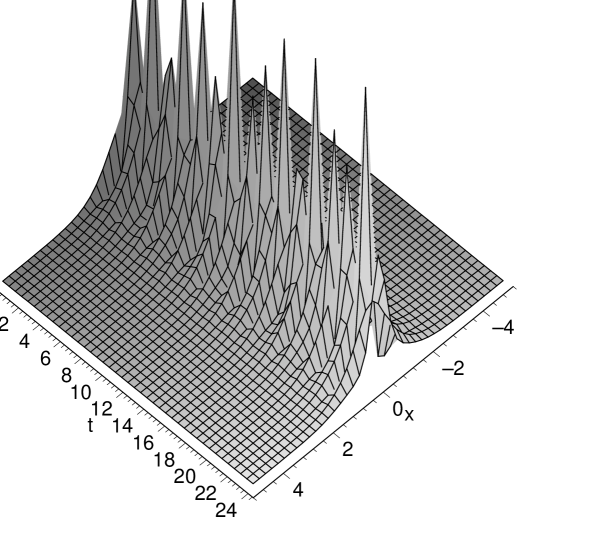
Figure 1: Square of module of the MNSE breather solution (16) for $w_{1}=1/3$, $w_{2}=1$ and $\alpha=0.1$.

Acknowledgements

The author is grateful to the Organizing Committee of the conference GIN’01 (Bansko, Bulgaria) for financial support. Stimulating discussions with Prof. V.S. Gerdjikov and Dr. V.S. Shchesnovich are greatly appreciated. The author thanks V.S. Shchesnovich for invaluable help with the illustrative material. This work was partly supported by grant no. 97-2018 from INTAS-Belarus.

References

[1]
Hasegawa A. and Tappert F., Appl. Phys. Lett. 23 (1973)
142.
[8]
Rangwala A. and Rao J.A., J. Math. Phys. 31 (1990) 1126.
[9]
Anderson D. and Lisak M., Phys. Rev. A 27 (1983) 1393.
[10]
Satsuma J. and Yadjima N., Progr. Theor. Phys. Suppl. 55
(1974) 284.
[11]
Golovchenko E. et al., Doklady AN SSSR 288 (1986) 851.
[12]
Ohkuma K., Ichikawa Y.H., and Abe Y., Opt. Lett. 12
(1987) 516.
[13]
Novikov S.P., Manakov S.V., Pitaevski L.P., and Zakharov V.E.,
Theory of Solitons. The Inverse Scattering Method
(Consultant Bureau, New York 1984).
[14]
Shchesnovich V.S. and Doktorov E.V., Physica D 129
(1999) 115.