Interaction of a discrete breather with a lattice junction

Abstract

We study the scattering of a moving discrete breather (DB) on a junction in a Fermi-Pasta-Ulam (FPU) chain consisting of two segments with different masses of the particles. We consider four distinct cases: (i) a light-heavy (abrupt) junction in which the DB impinges on the junction from the segment with lighter mass, (ii) a heavy-light junction, (iii) an up mass-ramp in which the mass in the heavier segment increases continuously as one moves away from the junction point, and (iv) a down mass-ramp. Depending on the mass difference and DB characteristics (frequency and velocity), the DB can either reflect from, or transmit through, or get trapped at the junction or on the ramp. For the heavy-light junction, the DB can even split at the junction into a reflected and a transmitted DB. The latter is found to subsequently split into two or more DBs. For the down mass-ramp the DB gets accelerated in several stages, with accompanying radiation (phonons). These results are rationalized by calculating the Peierls-Nabarro barrier for the various cases. We also point out implications of our results in realistic situations such as electron-phonon coupled chains.

I Introduction

Static discrete breathers (DB) are time-periodic, persistent, intrinsic localized exact modes in nonlinear lattices. Rigorous proofs of their existence have been obtained and systematic studies of their properties were carried out using various (approximate) complementary approaches, see e.g. [Flach1998, ] for an overview. In contrast, as first noticed in numerical investigations and then justified theoretically, moving DBs exist as approximate solutions in nonlinear lattices, both Hamiltonian and non-Hamiltonian (with dissipation and periodic forcing). These solutions are known to be rather stable (i.e., long-lived) and have been an object of constant investigation during the last decade, see [moving, ] for a non-exhaustive list.

Different physical systems in which there are realizations of (moving) DBs include conjugated polymers [kress, ; avn2, ], charge-density-wave materials (e.g., metal-halogen electronic chains [avn3, ]), Josephson ladders [avn4, ], coupled electron-vibron lattice systems [hennig, ] and spin chains [spin, ]. Sputtering on crystal surfaces and damage tracks in certain mica minerals have also been attributed to moving breathers [mica, ]. Experimentally, breathers have been probed by ultrafast resonance Raman [avn3, ] and inelastic neutron scattering [fillaux, ] among other techniques.

In a recent series of papers [impurity, ], the problem of the interaction of a moving DB with an impurity was addressed in the case of a lattice with nonlinear on-site potential and harmonic first-neighbor coupling. As it was shown, this interaction can lead to reflection, transmission or trapping of the DB at the impurity, depending on the initial velocity, amplitude and phase of the DB, as well as on the ‘strength’ and spatial extent of the impurity.

Our objective here is to investigate the scattering of a DB at a junction in a (nonlinear) FPU chain consisting of two segments that are “slightly different”–i.e., for instance, with different interaction parameters or with different masses of the particles in the two segments. The reason for choosing the FPU chain is simple. It has historically provided a testbed for exploring novel nonlinear phenomena in discrete systems. In addition, it is one of the simplest nonlinear (polynomial) potentials amenable to some analytical calculations.

Our preliminary numerical simulations indicate that these two types of problems are not qualitatively very different. Therefore, here we will concentrate exclusively on the second type of configuration, the one with slightly different masses on the two sides of the chain. A physical realization of this configuration could be in low-dimensional electronic materials with different electron-phonon coupling or two segments with different isotopes (e.g., carbon isotopes in conjugated polymers [kress, ; avn2, ] and platinum isotopes in metal-halogen chains [avn3, ]), Josephson-Junction arrays [avn4, ] with dissimilar interaction strengths, optical fibers with two different refractive indices [agrawal, ], etc. We note that the scattering of Toda solitons at a mass interface was studied previously [mertens1, ]. To the best of our knowledge, the scattering of a DB at such an interface has not yet been investigated.

The paper is organized as follows. In Sec. II we present the details of the FPU model in a homogeneous chain, an estimate of the Peierls-Nabarro barrier for moving DBs, and finally, some details on the numerical initialization of a moving DB. Section III contains results for both the light-heavy and the heavy-light mass junction, where we elaborate on the reflection and transmission (and eventually on the splitting) of the DB. Interaction of the DB with both the up mass-ramp and the down mass-ramp is discussed in Sec. IV, where we explore DB reflection (with eventual trapping) and acceleration (with eventual splitting). In Sec. V we summarize our main findings and enumerate some of the open questions. Details of the Peierls-Nabarro barrier calculation, using a new perturbative technique, for the various homogeneous and inhomogeneous cases are relegated to an Appendix.

II The model

II.1 The FPU model

The FPU model represents a one-dimensional (1D) chain of particles with no on-site potential (i.e., an acoustic chain), with the Hamiltonian

$$H = \sum_{n}\left[\frac{m\dot{x}_{n}^{2}}{2}+\frac{\alpha}{2}(x_{n+1}-x_{n}-a)^{2}\right.$$ (1)

$$+ \left.\frac{\beta}{4}(x_{n+1}-x_{n}-a)^{4}\right]\,,$$

where $\alpha$ and $\beta$ denote, respectively, the strengths of the linear and nonlinear nearest-neighbor interactions; $a$ represents the lattice constant (i.e., the equilibrium distance $a=x_{n}^{eq}-x_{n-1}^{eq}$ between neighboring sites), and $m$ is the mass of the particles. For simplicity, all these quantities (and those we will introduce later) are expressed in dimensionless units. The corresponding equation of motion for a generic particle is:

$$m\ddot{x}_{n} = \alpha\,(x_{n+1}+x_{n-1}-2x_{n})\,+\,\beta\,[(x_{n}-x_{n-1}-a)^{3}$$ (2)

$$- (x_{n+1}-x_{n}-a)^{3}]\,.$$

In terms of the elongations $u_{n}=x_{n}-x_{n}^{eq}$, it becomes:

$$m\ddot{u}_{n} = \alpha\,(u_{n+1}+u_{n-1}-2u_{n})\,+\,\beta\,[(u_{n}-u_{n-1})^{3}$$ (3)

$$- (u_{n+1}-u_{n})^{3}]\,,$$

or, by introducing the relative elongations of neighboring sites

$$\tau_{n}=(x_{n}-x_{n}^{eq})-(x_{n-1}-x_{n-1}^{eq})=x_{n}-x_{n-1}-a\,,$$ (4)

$$m\ddot{\tau}_{n}=\alpha\,(\tau_{n+1}+\tau_{n-1}-2\tau_{n})\,+\,\beta\,(\tau_{n+1}^{3}+\tau_{n-1}^{3}-2\tau_{n}^{3})\,.$$ (5)

As it was shown (see, for example [Flach1998, ] for an overview, and references therein, and [James2001, ]), the FPU lattice admits DB-like solutions (stationary, localized, time-periodic modes) with periods $T_{DB}$ that are smaller than the minimum period of the phonon spectrum, i.e.,

$$T_{DB}<\pi\,\sqrt{m/\alpha}\,.$$ (6)

Also, as shown, for example in [Page1990, ] and [Sandusky1992, ], the most localized of these modes are an odd-type mode with an “approximate” pattern of the amplitudes of the elongations $u_{n}$ of the form: $A_{odd}(...,0,-1/2,1,1/2,0,...)$, and an even-type mode [footnote1, ] : $A_{even}(...,0,-1,1,0,...)$. The amplitudes $A$ are determined by the interaction constants $\alpha$ and $\beta$ and by DB’s frequency $\omega_{DB}=2\pi/T_{DB}$. For given interaction constants, the $A$’s decrease with increasing $T_{DB}$. On the contrary, keeping $T_{DB}$ fixed and decreasing the interaction constants generally leads to an increase in the amplitudes $A$. By “approximate” above we mean that (as seen in [Sandusky1992, ]) these patterns are exact only for a pure even-order anharmonic lattice in the limit of increasing order of anharmonicity. Nevertheless, only minor corrections are needed in order to make these patterns ‘more precise’ solutions of the FPU lattice, their symmetry being preserved. Mainly, these corrections refer to the fact that the DB can extend over more than three, and two sites, respectively, for odd and even modes. Although, in theory, a DB has an infinite extension [with an exponential decay of the amplitude of the relative elongation as one moves far away from the center (maximum amplitude sites) of the DB], in practice, however, one can restrict the analysis to five, and four sites, respectively, for the two types of modes of the DB mentioned above.

To evaluate the relative elongations for the two configurations, and their corresponding energies, we introduced a simple perturbative technique that uses the ratio between the square of the maximum phonon frequency and the square of the DB frequency as the perturbation parameter:

$$\varepsilon=\frac{4\alpha}{m\,\omega_{DB}^{2}}\,,$$ (7)

combined with a rotating wave approximation, RWA (see, e.g., [Flach1998, ] and references therein). The results of our calculations, presented below and, in more detail, in the Appendix, can be compared with the numerical results of Green’s function method (that is also based on RWA). For example, for the even-symmetry mode, our calculations [up to ${\cal O}(\varepsilon^{2})$] agree generally up to an error of no more than $4\%$ with the results of [Sievers1988, ] obtained with Green’s function method. The error in evaluating the configurations (as compared with the results of the exact numerical method of the analytical continuation from the anticontinuous limit [Aubry, ]) is essentially connected with the limitations of RWA, and therefore becomes progressively smaller for ‘heavier’ DBs, i.e., DBs that are progressively further away (in frequency) from the phonon band limit.

The primary ingredients of the analytic method are the ansatz concerning the temporal evolution of particles’ elongations:

$$u_{n}(t)=A\xi_{n}\cos(\omega_{DB}t)\,,$$ (8)

(where $A$ and $\xi_{n}$ are the amplitude and the shape function, respectively), together with the RWA that entails neglecting higher-frequency harmonics [i.e., $\cos^{3}(\omega_{DB}t)\approx(3/4)\cos(\omega_{DB}t)$]. Including these elements in Eq. (3), one obtains an infinite set of nonlinear coupled equations for the shape function:

$$m\omega_{DB}^{2}\xi_{n} = \alpha(2\xi_{n}-\xi_{n+1}-\xi_{n-1})$$ (9)

$$+ \frac{3}{4}\beta A^{2}[(\xi_{n}-\xi_{n+1})^{3}+(\xi_{n}-\xi_{n-1})^{3}]\,.$$

Or, in terms of the relative elongations:

$$\tau_{n}(t)=A\zeta_{n}\cos(\omega_{DB}t)\,,\,\,\,\zeta_{n}=\xi_{n}-\xi_{n-1}\,,$$ (10)

$$m\omega_{DB}^{2}\zeta_{n} = \alpha(2\zeta_{n}-\zeta_{n+1}-\zeta_{n-1})$$ (11)

$$+ \frac{3}{4}\beta A^{2}(2{\zeta_{n}}^{3}-{\zeta_{n+1}}^{3}-{\zeta_{n-1}}^{3})\,\,.$$

Next, we consider the following expansion of the shape function in terms of the small parameter $\varepsilon$, see Eq. (7):

$$\xi_{n}=\xi_{n}^{(0)}+\varepsilon\xi_{n}^{(1)}+\varepsilon^{2}\xi_{n}^{(2)}+...$$ (12)

and then proceed through the usual steps of a perturbative calculation. For details of these calculations, refer to the Appendix.

II.1.1 The Peierls-Nabarro barrier for the homogeneous FPU chain

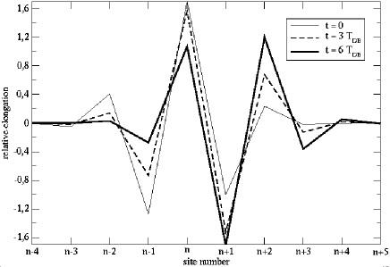
(a) homogeneous chain

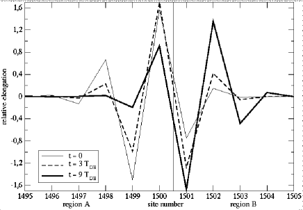
(b) light-heavy junction, $m_{B}=1.002$: transmission of the DB

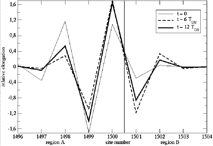
(c) light-heavy junction, $m_{B}=1.04$: reflection of the DB

Figure 1: Temporal evolution of a DB’s configuration in three different situations. Notice the alternation between odd and even- type configurations. $T_{DB}=2.1$.

As illustrated in Fig. 1(a) on an actual example, the DB translates from one lattice site to another by continuously deforming its shape, alternately, between an odd-type of configuration and an even-type one. Therefore, in a discrete lattice there is an energy cost associated with moving a nonlinear localized mode by a lattice constant–this represents the so-called Peierls-Nabarro barrier (PNB), see [PNBARRIER, ]. It can be estimated by calculating the energy difference between even- and odd-type configurations. The results presented in the Appendix allow us to evaluate the PNB in an homogeneous chain (i.e., all particles with same $\alpha$, $\beta$, and $m$):

$$\Delta E_{PN}^{h} = E_{odd}^{h}-E_{even}^{h}=m\omega_{DB}^{2}\left(\frac{\alpha}{\beta}\right)\left[{0.00836}\,{\varepsilon}^{-1}\right.$$ (13)

$$-\,\left.0.00765-0.01827\,\varepsilon+{\cal O}(\varepsilon^{2})\right]\,,$$

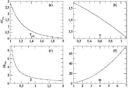
Figure 2: Variation of the Peierls-Nabarro barrier as a function of breather time period ($T_{DB}$), FPU chain parameters ($\alpha$, $\beta$) and mass ($m$). (a) $\alpha=1$, $\beta=1$, $m=1$. (b) $T_{DB}=1.2$, $\beta=1$, $m=1$. (c) $\alpha=1$, $T_{DB}=1.2$, $m=1$. (d) $\alpha=1$, $\beta=1$, $T_{DB}=1.2$.

where the superscript $h$ refers to the homogeneous case. As expected, it is a very small energy barrier (as compared with the one typically found in some optical chains, i.e., chains with on-site nonlinear potential, see [PNBARRIER, ]); for example, for a very heavy DB, $\Delta E_{PN}^{h}/E_{odd}^{h}\sim 2.1\%$ only! This explains the well-known fact that it is rather easy to create mobile DBs in an FPU chain, and also why in the first-order approximation in [McKay2002, ] this barrier was found to be zero. In Fig. 2 we represent the dependence of the barrier on various parameters: (i) DB’s period $T_{DB}$ (as expected, also see below the discussion on the generation of moving DBs, the PNB is larger for higher-frequency DBs; in the first order of the perturbative expansion, PNB varies as $1/T_{DB}^{4}$). (ii) $\alpha$ and (iii) $\beta$. At the first order in the perturbational expansion, the PNB does not depend on $\alpha$, but only on $1/\beta$, i.e., it decreases with increasing nonlinearity. This feature can be easily understood if one views the role of the nonlinearity as reducing particles’ excursions around equilibrium, and therefore reducing the differences between the odd- and even-parity configurations, i.e., the PNB. (iv) Finally, on $m$ (note that, in the first order of the perturbative expansion, the PNB varies as $m^{2}$).

II.2 DB generation and initialization

For simulation purposes, the static DBs were generated numerically in the homogeneous FPU chain using the extremely fast algebraic method recently introduced by Tsironis [Tsironis2002, ]. As shown in [Tsironis2002, ], this method, although approximate, is generally more accurate than the RWA and agrees with the exact results of the anticontinuous limit method (which requires much longer computational times, see [Aubry, ]) typically to $1\%$ or even better.

In order to move these breathers, we used a simple approximation of the systematic pinning mode excitation method of Chen et al. [Chen1996, ]. Namely, we ‘kick’ initially the DB by assigning to the points of the lattice initial relative velocities that are a fraction $\lambda$ (the “kicking coefficient”) of the gradient of $|\tau_{n}|$, i.e.,

$$\dot{\tau_{n}}(t=0)=\lambda\,(|\tau_{n+1}|-|\tau_{n-1}|)/2\,\,.$$ (14)

Note that this method is not so different from the ‘more empirical’ methods used in [Sandusky1992, ] to obtain moving DBs. We notice that, when starting to move, the DB first loses, through phonon radiation in the lattice, a large part of the kinetic energy we assigned to it when kicking. The rest of the received energy is used to overcome the Peierls-Nabarro barrier, and, as already mentioned, the DB moves from one lattice site to another by a continuous alternation between odd- and even- type configurations.

This alternation between the two types of configurations for a moving DB can be noticed when inspecting the temporal evolution of the potential (or kinetic) energy of the DB. Indeed, the envelope of the temporal oscillations of DB’s potential (kinetic) energy presents a series of periodically alternating relative maxima and minima, indicating the alternation between these configurations. The period between two such successive maxima (or minima) gives a rough estimate of the time needed by the DB to move from one site to another. But no more than a “rough estimate”, because (i) the real time a DB takes for this movement does not bear a commensurability relation with $T_{DB}$, and (ii) the structure of the envelope is more complex, due to the presence of other “secondary” frequencies of the DB (see [Flach1998, ], and the discussion in Sec. V), and (iii) there are some “imperfections” in this periodic behavior of the envelope, that are connected to the existence of a rather irregular time dependence of the relative phases of two neighboring sites (already mentioned in [Sandusky1992, ]). Probably, this is ultimately related to the non-exact character of a moving DB as a solution of the Hamiltonian lattice. Note also that a moving DB constantly loses energy while moving through the lattice, although at a very small ‘dissipation rate’. For example, as also shown in [Ibanes2002, ], for a DB moving in a uniform lattice, this energy decrease, if fitted to an exponential, corresponds to a decay rate on the order of $\sim 10^{-6}$/unit time. This rate is higher for the faster DBs. Also, as explained in detail by the same authors, the analysis of the temporal behavior (and, in particular, of the extremal points) of the kinetic and potential energy allows one to evaluate the translational energy of a moving DB, which was found to be at most $1\%$ of the total energy of the DB. Not surprisingly, this value is of the same order of magnitude as the Peierls-Nabarro barrier.

Returning to the kicking method for moving a DB, we make several other remarks. First that, as previously noticed (see, e.g., [Dauxois1993, ]), the ‘light’ DB’s (i.e., those that are relatively not too far in frequency above the phonon band limit) are definitely easier to move than the ‘heavy’ DBs (which are, by comparison, much more localized and therefore much more sensitive to the discreteness of the lattice). In terms of the initial kick, this means that the minimum value of the kicking coefficient, $\lambda$, for which one gets an essentially regular motion of the DB [footnote2, ] is larger for ‘heavier’ DBs. Also, one notices that, in general, the velocity of the moving DB obtained through this kicking method seems first to increase with increasing $\lambda$, and after that it reaches a certain ‘saturation value’, i.e., it does no longer increase with $\lambda$, but keeps a constant value. This leads to a rather narrow window of the possible values of the DB velocities, which is somewhere around a tenth of the phonon’s velocity (for example, for $\alpha=\beta=1$, a lattice constant $a=10$, and for a DB of period $T_{DB}=2.1$, the values of the velocities belong to a window of $\approx[0.35,1.25]$; note that the sound velocity corresponds to $10$ in the dimensionless units). In the simulations we used a chain with the first and last point held fixed (i.e., fixed boundary conditions; this should not raise conceptual problems, as such points correspond to $m\rightarrow\infty$). Also, we tried to avoid the interference between the observed phenomena and the phonons that reflect on these fixed edges–and for this purpose we generally used sufficiently long chains (so that the reflected phonons do not come back to the interesting central regions during the observation period).

III Interaction of a DB with a junction

We now address the main problem in this paper. Consider the junction between two semi-infinite FPU chains (let us call them “A” and “B”, respectively, with the corresponding subscripts for their characteristic parameters). We fix the parameters of the A chain $\alpha_{A}$, $\beta_{A}$, and $m_{A}$. For the B chain, we will fix the interaction parameters identical to those of the A chain,

$$\alpha_{B}=\alpha_{A}\,\,,\,\,\,\,\,\,\beta_{B}=\beta_{A}\,,$$ (15)

and vary the mass of the particles, $m_{B}$. Note that in all the numerical simulations we set $\alpha_{A}=\beta_{A}=1$, as well as $m_{A}=~{}1$.

A DB is generated in the A part of the chain and is sent to the junction with the B part. Depending on the difference between the masses of the particles in the two parts of the chain, the DB exhibits different behaviors at the junction.

III.1 The Peierls-Nabarro barrier at the junction

In order to understand and predict the behavior of a moving DB at such a junction, the first step is to study the change in the Peierls-Nabarro barrier at the junction. Namely, to determine what would be the equivalent of the odd- and even- type configurations at the junction, and what would be the corresponding difference in the configurational energy. Note that in the case of an inhomogeneous chain the PNB is defined as the difference between the global maximum and the global minimum of the configurational energy. We consider the case when $\delta=(m_{B}-m_{A})/m_{A}$ is a small quantity, that we use as a perturbation parameter for evaluating the changes in the odd and even configurations at the junction. Thus, we consider a “double” perturbation expansion of particles’ envelope function:

$$\xi_{n} = (\xi_{n,0}^{(0)}+\varepsilon_{A}\xi_{n,0}^{(1)}+\varepsilon_{A}^{2}\xi_{n,0}^{(2)}+...)$$ (16)

$$+ \delta\,\,(\xi_{n,1}^{(0)}+\varepsilon_{A}\xi_{n,1}^{(1)}+\varepsilon_{A}^{2}\xi_{n,1}^{(2)}+...)$$

$$+ \delta^{2}\,\,(\xi_{n,2}^{(0)}+\varepsilon_{A}\xi_{n,2}^{(1)}+\varepsilon_{A}^{2}\xi_{n,2}^{(2)}+...)+...\,,$$

where $\varepsilon_{A}$ is evaluated with respect to the parameters of the A chain, i.e.,

$$\varepsilon_{A}=\frac{4\alpha_{A}}{m_{A}\,\omega_{DB}^{2}}\,,$$ (17)

Corresponding to the different configurations it has to exhibit in order to traverse the junction, the DB encounters three new energy barriers (refer to the Appendix for more details). These are, in the order of their appearance as the DB moves through the junction:

$$\Delta E_{PN}^{j(I)} = \Delta E_{PN}^{h(A)}+m_{A}\omega_{DB}^{2}\left(\frac{\alpha_{A}}{\beta_{A}}\right)\times$$ (18)

$$\times\left[\delta\left(0.13793\,\varepsilon_{A}^{-1}-0.01573+0.0056\,\varepsilon_{A}\right)\right.$$

$$\left.+\delta^{2}\left(0.49933\,\varepsilon_{A}^{-1}+0.21657-0.69346\,\varepsilon_{A}\right)\right].$$

This energy barrier corresponds to the difference between the energy of the odd-type configuration I in the Appendix–for which the site of maximum elongation is the last site in the part A of the chain–and the energy of the even-type configuration in the homogeneous A chain.

$$\Delta E_{PN}^{j(II)} = \Delta E_{PN}^{h(A)}+m_{A}\omega_{DB}^{2}\left(\frac{\alpha_{A}}{\beta_{A}}\right)\times$$ (19)

$$\times\left[\delta\left(0.64113\,\varepsilon_{A}^{-1}-0.14880-0.00526\,\varepsilon_{A}\right)\right.$$

$$\left.+\delta^{2}\left(0.75093\,\varepsilon_{A}^{-1}+0.21657-0.68820\,\varepsilon_{A}\right)\right].$$

This energy barrier corresponds to the difference between the energy of the odd-type configuration III in the Appendix–for which the site of maximum elongation is now the first site in the part B of the chain–and the energy of the even-type configuration in the homogeneous A chain). The last PNB barrier is associated with the difference between the energy of the odd-type configuration in the homogeneous B chain and the even-type configuration in the homogeneous A chain:

$$\Delta E_{PN}^{j(III)} = \Delta E_{PN}^{h(A)}+m_{A}\omega_{DB}^{2}\left(\frac{\alpha_{A}}{\beta_{A}}\right)$$ (20)

$$\times\left[\delta\left(0.77906\,\varepsilon_{A}^{-1}-0.16470\right)\right.\left.+\delta^{2}\left(0.38953\,\varepsilon_{A}^{-1}\right)\right]\,.$$

Here $\Delta E_{PN}^{h(A)}$ denotes the Peierls-Nabarro barrier in the homogeneous A chain, and $j$ refers to the junction.

Note that for a heavy-light junction, i.e., for $\delta<0$, these barriers are smaller than the PNB barrier in the homogeneous A part of the chain and therefore a DB that moves smoothly in region A will have no ‘energetic difficulties’ to enter region B. On the contrary, for a light-heavy junction, i.e., for $\delta>0$, these barriers are larger than the PNB in part A of the chain and one sees that, at the dominant orders in $\varepsilon_{A}$ and $\delta$, they increase in succession. Therefore, there appears the possibility that a DB that arrives at such a junction cannot overcome either the first, or the second , or the third barrier. The presence of these barriers is confirmed by numerical simulations (through fine tuning of $m_{B}$).

III.2 The light-heavy junction

We first present the generic results of our simulations for this case.

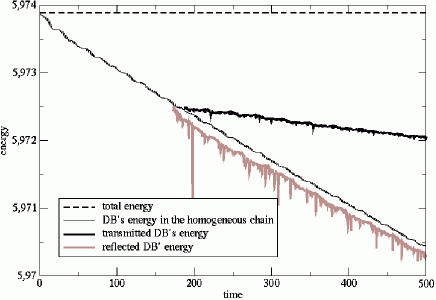
Figure 3: Energy of the DB for the three cases in Fig. 1.

(a) A DB can continue its movement into region B. Its frequency is not (detectably) modified. The DB keeps on losing energy in region A as well as in region B, but at a smaller rate in region B, see Fig. 3. This might be connected to the fact that (given that it keeps essentially the same frequency) the DB is further away from the phonon band limit in region B than in region A. Also, its velocity in region B is smaller than in region A. This is related to the fact that a part of the “extra” energy that in region A corresponded to its movement as a whole (with a velocity $v_{A}$) is now used for the new, higher mean configurational energy, and also to overcome the correspondingly higher Peierls-Nabarro barrier in region B. Therefore, the “extra” kinetic energy, and correspondingly the velocity $v_{B}$ in region B are smaller than in region A.

(b) The DB can reflect at the junction and return to the region A. Its frequency and energy (see Fig. 3) are not sensitively modified by this reflection, and neither its velocity (that only changes sign).

These observations can be explained qualitatively on the basis of the results presented above for the PNB that a DB (that keeps a constant period $T_{DB}$) has to overcome in order to continue its movement in region B. The main conclusion is that for a DB arriving at the junction, there exists a critical value of the mass $m_{B}=m_{crit}^{j}$ above which the DB cannot penetrate in region B and is reflected to region A. This critical value depends on the frequency of the DB, namely it increases with decreasing $T_{DB}$ (i.e., it is larger for heavier DBs). However, it also depends on the velocity the DB has in region A: it increases with increasing $v_{A}$ (i.e., a more rapid breather needs a larger mass $m_{crit}^{j}$ to be reflected than a slower DB of the same frequency). This can be readily understood: a more rapid DB in region A has more “extra” energy (above the Peierls-Nabarro barrier $\Delta E_{PN}^{h(A)}$) than a slower one. Therefore, it may use this energy to overcome the Peierls-Nabarro barrier at the junction and to penetrate in region B, while a slower DB cannot overcome the junction barrier.

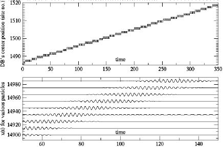
(a) homogeneous chain

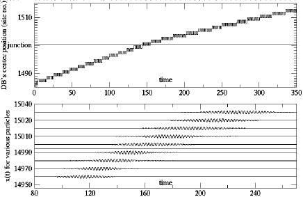
(b) light-heavy junction, $m_{B}=1.002$: transmission of the DB

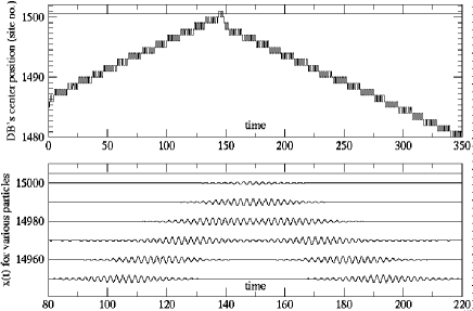
(c) light-heavy junction, $m_{B}=1.04$: reflection of the DB

Figure 4: Propagation, transmission and reflection of the DB for the three situations in Fig. 1. The associated motion of particles in the region of the DB is also shown. $T_{DB}=2.1$.

We present below two comparative sets of pictures of the cases when a given DB (a) moves in a homogeneous chain, (b) passes through a light-heavy junction, and (c) is reflected at the light-heavy junction. Fig. 1 shows the temporal evolution of the configurations of the DB in these three situations, while Fig. 4 shows the movement of DB’s center along the chain, and also the temporal evolution of the elongations of various particles affected by the DB.

III.3 The heavy-light junction

As already mentioned above, given that the PNB decreases at a junction with $m_{B}<m_{A}$ , one can naively predict that the DB will always penetrate and continue to move in region B without any hinderance. Numerical simulations show that this is indeed the case–at least as long as the difference between $m_{B}$ and $m_{A}$ is sufficiently small. For example, in the particular case of $m_{B}=0.99$ (recall that in simulations we took $m_{A}=1$) we studied the dependence of the characteristics of the ‘transmitted’ DB on those of the ‘incident’ one. First of all, one notices that the transmitted breather takes some time to “adjust” to the new environment (and ‘heavier’ DBs take a longer time to adjust than the ‘lighter’ ones). During this period, the DB loses energy and adjusts its final energy to the smaller mass of region B.

The transmitted DB (within estimated errors) has the same period as the incident one (i.e., the adjustment is such that it preserves DB’s frequency). After this transient period, the DB reaches a constant ‘asymptotic’ velocity. In general, there is no simple relationship between this asymptotic velocity $v_{B}$ and the characteristics of the incident DB, namely its initial velocity (in region A) $v_{A}$ and its period $T_{DB}$.

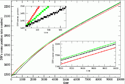
Figure 5: A heavy–light ($m_{B}=0.99$) junction. For various initial velocities $v_{A}$ of a DB with a given period ($T_{DB}=2.1$) one gets approximately the same asymptotic velocity $v_{B}$ in region B (see the lower inset). The upper inset depicts the DB’s position at very early time before reaching the junction, while the lower inset depicts the DB’s asymptotic trajectory.

However, there is a tendency towards ‘uniform’ velocities after transmission through the junction for a given DB. Namely, for a DB with period $T_{DB}$ and different velocities in region A, $v_{A}$, the effect of entering region B is to reduce the dispersion of these velocities, i.e., the dispersion of the asymptotic velocities, $v_{B}$, is smaller [footnote3, ]. This observation is illustrated in Fig. 5 for a given DB (with $T_{DB}=2.1$) and for three representative initial velocities $v_{A}$ (chosen, respectively, as the lower and upper limits of the velocities that could be obtained through the “kicking” method described above in Sec. II.2, and one value in-between these limits).

It was relatively more difficult to investigate the dependence of the asymptotic velocity $v_{B}$ on DB’s period $T_{DB}$, simply because it is rather difficult with the kicking method to obtain the same velocity for DBs of different frequencies. However, we managed to obtain four DBs of periods varying between $2.2$ and $2.5$ (with a step $0.1$) and almost (within $4\%$) the same initial velocity. The simulations show no simple monotonic dependence of $v_{B}$ on $T_{DB}$.

Next, we focus on the most important part of this section (that will clarify the meaning of sufficiently small difference between $m_{B}$ and $m_{A}$). Specifically, how does the behavior of a given DB depend on the value of $m_{B}$? To analyze this, we ran systematic simulations for a given DB (we chose one with $T_{DB}=2.1$ and an initial velocity $v_{A}=0.928$, that corresponds to a kicking coefficient $\lambda=0.7$), and for various values of $m_{B}$. The behavior of the DB at the junction is rather complex, and can be described essentially as follows: the DB, entering the region of lower mass, has “extra” energy. During an “adjusting period” (that might take from about ten to hundred DB periods), this extra energy is redistributed between: (i) the kinetic energy of DB’s translation as a whole (the DB is accelerated upon entering region B); (ii) perturbations (which we address later) in the A and also in the B part of the chain; and (iii) a slight decrease of transmitted DB’s period (i.e., increase of its configurational energy). The redistribution of energy between these elements is a delicate process, and it depends on the mass difference between regions A and B. When the mass difference is sufficiently small, up to, say, $(m_{A}-m_{B})/m_{A}=0.4$, the predominant phenomena are (i) and (ii)–the perturbations being small-amplitude ones, i.e., phonons that move rapidly far away from the junction, in both A and B part.

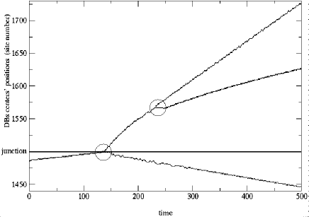
Figure 6: A heavy–light ($m_{B}=0.50$) junction. An initial DB ($T_{DB}=2.1$) splits into a reflected and a transmitted DB. Later on, the transmitted DB furhter splits into two other DBs (the circles on the figure indicate the regions of the splittings). Note that when the mass difference is even larger, the transmitted DB (that has progressively less energy) might split into three or even four smaller DBs. Decreasing $m_{B}$ furhter leads practically to the disappearance of the transmitted DB, and to a substantial phonon creation.

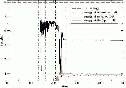
Figure 7: The energy associated with the phenomena described in Fig. 6. The dashed-dotted lines on the figure delimit the intervals of the occurrence of the splitting phenomena, when there is no net separation between the resulting DBs, i.e., no clear separation of their energies.

When the mass difference is even larger, we find that in A part there are not simply phonons that appear, but a reflected DB: the initial DB, arriving at the junction, is split into a reflected DB and a transmitted one. Moreover, the transmitted DB is usually (nonlinearly) unstable and subsequently splits into two (or sometimes more) other DBs. See Fig. 6 for a realization of these phenomena: the trajectory of the initial DB, the reflected one, the transmitted DB and its subsequent splitting into two other DBs. Figure 7 offers the energy variation associated with these phenomena. We note that the total energies of the resulting DBs never sum up to the initial energy due to the phonon losses in the chain that accompany all these processes. To our knowledge, such DB splitting has not been noticed before. If we continue to decrease $m_{B}$, the reflected DB (that is initially very weak energetically as compared to the transmitted one) becomes progressively more energetic, while the transmitted DB becomes progressively weaker and finally dissappears in region B leaving only rapidly-moving phonons in its wake. The end product is the “strong” (i.e., large-amplitude) reflected DB in region A.

IV Interaction of a DB with a ‘mass ramp’

IV.1 The Peierls-Nabarro barrier for a ‘ramp’

Consider that in region B the mass of the particles varies slightly, linearly, as one moves away from the junction point, i.e., the mass of the $k$-th particle in B part is

$$m_{B}(k)=m_{A}(1+k\Delta)\,,$$ (21)

where $\Delta>0$ corresponds to an up mass-ramp, while $\Delta<0$ to a down mass-ramp, and for analytic calculation purposes we consider that $|\Delta|\ll 1$. A double analytical expansion in $\varepsilon_{A}$ and $\Delta$ allows us to estimate the shape function for the equivalents of the odd- and even-type configurations, and therefore to estimate the Peierls-Nabarro barrier the DB must overcome in order to move up to site $k$ in region B. The barrier (with details given in the Appendix) is found to be:

$$\Delta E_{PN}^{r}(k) = E_{odd}^{r}(k)-E_{even}^{h(A)}=\Delta E_{PN}^{h(A)}$$ (22)

$$+m_{A}\omega_{DB}^{2}\left(\frac{\alpha_{A}}{\beta_{A}}\right)\left\{\Delta\left[(0.77906k+0.77906)\,\varepsilon_{A}^{-1}\right.\right.$$

$$\left.\left.-(0.16470k+0.16470)\right]\right.$$

$$\left.+\Delta^{2}\left[(0.38953k^{2}+0.77906k+2.56207)\,\varepsilon_{A}^{-1}\right.\right.$$

$$\left.\left.+0.91605-3.2585\varepsilon_{A}\right]\right\}\,,$$

where the superscript $r$ refers to the ramp.

IV.2 The ‘up-ramp’

This corresponds to the case $\Delta>0$. The main result is that a DB that enters the B part of the chain is finally reflected (at some point within the B chain) and returns to part A. Note that:

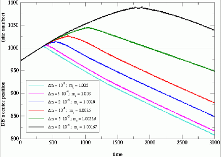
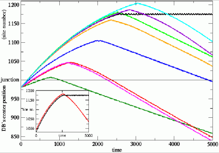
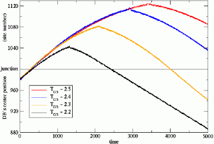
Figure 8: The behavior of a DB on an up-ramp depending on (a) the slope of the ramp ($T_{DB}=2.1$) and (b) its initial velocity $v_{A}$. Note that the DB can also get trapped on the ramp; but, as shown in the inset, a slight perturbation–for example, a slight modification of the initial conditions–can lead to the disappearance of trapping. ($T_{DB}=~{}2.1$). (c) The behavior of a DB as a function of the period $T_{DB}$ of the DB. (Note the limited possibilities to obtain DBs of various periods with rigorously the same initial velocity $v_{A}$.)

(a) The point where the DB is reflected, i.e., the critical mass on the ramp, $m_{crit}^{r}$, depends on the ‘slope’ $\Delta$ of the ramp and is generally different from the value $m_{crit}^{j}$ that corresponds to the case of an abrupt junction, see Sec. III.2. This can be seen by equating the (critical values of the) most energetic odd-type configurations in B chain in the case of an abrupt junction and of a ramp, and finding the relationship between $m_{crit}^{j}$ and $m_{crit}^{r}$. In the particular case shown in Fig. 8, we note that the critical mass decreases with decreasing slope of the ramp and that it is smaller than the value for the junction case.

(b) For a given ramp, the critical mass increases with increasing initial velocity of a given DB (with a fixed frequency), see Fig. 8. Sometimes the DB can get trapped, as seen in the inset of this figure. Note, however, that if one changes slightly DB’s initial position in region A (without changing its initial velocity), then the DB is no longer trapped, but reflected, see the inset. Thus, trapping seems to be a rather delicate phenomenon, that depends on ‘how’ (i.e., with what precise configuration and relative phase difference between sites) the DB arrives at the trapping site.

(c) For a given ramp, the critical mass seems to increase with a decrease in DB’s period (i.e., it is larger for ‘heavier’ DBs for the same initial velocity), see Fig. 8. Note that in all these cases there is a typical temporal evolution of the energy of the DB. Before entering region B, one recognizes the usual small energy loss in an uniform FPU chain; then in the ramp part there is a somewhat smaller energy loss (presumably the DB is a little bit further away from the phonon band) that becomes progressively smaller when the DB is decelerated on the ramp. At a certain moment, the DB starts to ‘descend’ the ramp, to increase its velocity, and its energy loss increases progressively, again up to the usual loss in the homogeneous chain. When the DB ‘ascends’ the ramp, its configurational energy averaged over a period (and the corresponding Peierls-Nabarro barier) increase at the expense of its translational energy. Therefore, at a certain moment, the DB does no longer have sufficient “extra energy” to overcome the barrier and it is reflected (and sometimes it may get trapped). Rolling down the hill, it recuperates its translational energy and when it gets out from region B and re-enters region A it has almost the same velocity as its initial one in region A. The transmission and reflection are “almost elastic”, in fact the DB loses a little bit less energy than it loses normally during its movement in a uniform chain.

IV.3 The ‘down-ramp’

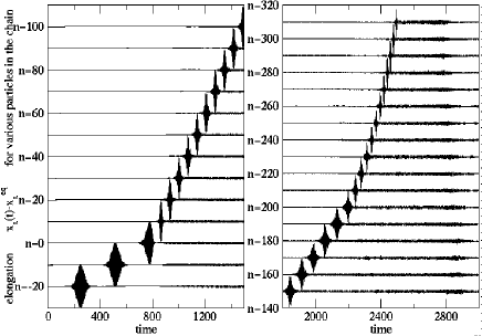
Figure 9: Acceleration of a DB on a down-ramp. Site n=0 corresponds to the last site in the region before the onset of the ramp. The slope of the ramp is $\delta=0.0018$. On the y axis we approached the sites by 9.9 lattice constants ($a=10$ units) in order to increase the resolution.

Consider now that in the region B the mass of the particles decreases from one particle to another with the small quantity $m_{A}\,\Delta<0$. An illustration of DB’s typical behavior is given in Fig. 9. As the DB enters the ramp it accelerates with a concomitant narrowing of its shape and the emission of some radiation (phonons). This is clearly seen as a change in slope (left panel). At later times we observe another change in slope signifying further acceleration of the DB with significant radiation and emission of smaller breathers (right panel). One can also observe other secondary, small-energy DBs that may form at later stages. Nonetheless, these phenomena are highly complex and beyond our current level of understanding.

V Conclusions and perspectives

We have systematically explored the transport properties of a discrete breather in a nonlinear chain comprising two segments with differing mass, specifically in an FPU chain. We considered abrupt junctions (light-heavy and heavy-light) as well as (up and down) mass ramps. We studied the trapping, reflection, transmission and splitting of the DB as a function of junction type, mass difference, breather frequency and velocity. The DB splitting, trapping and reflection may take place either at the junction or at a particular particle within the ramp. We also estimated the Peierls-Nabarro barrier for the different cases to understand the DB transport across a junction or within a ramp. However, the approach for calculating the PNB is based on the fundamental assumption that the period (frequency) of the DB does not change “significantly” during its movement, which has its limitations, as shown by the simulations and indicated above in various cases. Therefore, we can rely on this method only at a qualitative level.

In the present paper we exclusively focused on two segments with slightly different masses. It would be interesting to explore a junction (or ramp) between two segments with the same mass but with differing strength of either the harmonic ($\alpha$) or anharmonic ($\beta$) interaction parameter of the FPU chain. This is under investigation and our preliminary results do not demonstrate a qualitatively different picture compared to the mass case. In addition, if we consider an A–B–A mass sandwich structure then there is a distinct possibility that the breather will get trapped inside the B segment. By a suitable choice of the mass profile one may envision a ‘breather lens’. This is currently explored and preliminary results agree with these conjectures. We believe that our results are not specific to the FPU chain. Other nonlinear potentials should lead to generically similar results. Many open questions remain, e.g. better estimates for site-to-site traversal time of a DB, influence of the “secondary” frequencies of the DB on its behavior (for example, on the envelope of temporal oscillations of energy), a better understanding of the nonlinear instability that leads to DB splitting (reflected/transmitted, and afterwards to the secondary splitting of the transmitted DB), and consequently, to the complex behavior on a down-ramp, etc. An experimental realization of our findings in low-dimensional electron-phonon coupled materials [agrawal, ], e.g. conjugated polymers [kress, ; avn2, ] and metal-halogen chains [avn3, ], using different isotopes would be quite instructive in unraveling the interesting transport properties of breathers with potential applications.

VI Appendix: PNB for various configurations

In this appendix we present the relevant details of estimating the Peierls-Nabarro barrier for the different cases discussed in the text.

VI.1 The homogeneous chain

VI.1.1 The odd-type mode

It is characterized by $\xi_{n}=\xi_{-n}\equiv(-1)^{|}n|\eta_{n}$ ($\eta_{n}$, the reduced shape function, being positive for all $n$), together with the condition $\zeta_{0}=\eta_{0}=1$ (that gives the normalization of the shape function). The equations for the reduced shape function read, respectively:

$${\Lambda\varepsilon}=\frac{2-\varepsilon(1+\eta_{1})}{(1+\eta_{1})^{3}}\,\,,\mbox{for}\,\,\,n=0\,,$$

$$\eta_{n} = \frac{\varepsilon}{4}(2\eta_{n}+\eta_{n+1}+\eta_{n-1})+\frac{\Lambda\varepsilon}{4}[(\eta_{n}+\eta_{n+1})^{3}$$

$$+ (\eta_{n}+\eta_{n-1})^{3}]\,\,,\mbox{for}\,\,\,n\geq 1\,.$$

Here

$$\Lambda=\frac{3\beta A_{odd}^{2}}{4\alpha}\,.$$ (24)

Note the singular behavior in $\varepsilon^{-1}$ of the square of the amplitude, $A_{odd}^{2}$ (e.g., this means that the ‘heavier’ the DB, the larger its amplitude). Using the series expansions in $\varepsilon$ for $\xi_{n}$, Eq. (12), and the corresponding ones for the reduced shape function in Eq. (LABEL:etaodd), and ordering the corresponding powers of $\varepsilon$, one can show that the series $\eta_{n}^{(j)}$ (for a fixed $j$, i.e., for a fixed order in the perturbative expansion in $\varepsilon$) rapidly converges to zero with increasing $n$; more rapidly for the case of small $j$s than for larger ones [footnote4, ]. Finally, one is led to the following expressions for particles’ shape function:

$$\xi_{0}=1\,,$$

$$\xi_{1}=\xi_{-1}=(-1)[0.52305+0.15113\,\varepsilon+0.08549\,\varepsilon^{2}$$

$$\hskip 28.45274pt+{\cal O}(\varepsilon^{3})]\,,$$

$$\xi_{2}=\xi_{-2}=0.02305+0.15691\,\varepsilon+0.12643\,\varepsilon^{2}$$

$$\hskip 28.45274pt+{\cal O}(\varepsilon^{3})\,,$$

$$\xi_{3}=\xi_{-3}=(-1)[0.00580\,\varepsilon+0.04239\,\varepsilon^{2}$$

$$\hskip 28.45274pt+{\cal O}(\varepsilon^{3})]\,,$$

$$\xi_{n}={\cal O}(10^{-6})\,\,,\,|n|\geq 4\,\,,$$ (25)

together with the dependence of the amplitude $A_{odd}$ on DB’s frequency, mass $m$ of the particles (through $\varepsilon$), $\alpha$, and $\beta$:

$$\Lambda=\frac{3\beta A_{odd}^{2}}{4\alpha}={0.56609}\,{\varepsilon}^{-1}-0.59960+0.02366\,\varepsilon+{\cal O}(\varepsilon^{2})\,.$$ (26)

All these lead finally to the following expression for the configurational energy of the odd-parity mode:

$$E_{odd}^{h} = m\omega_{DB}^{2}\left(\frac{\alpha}{\beta}\right)[{0.38953}\,{\varepsilon}^{-1}-0.16470$$ (27)

$$- 0.12386\,\varepsilon+{\cal O}(\varepsilon^{2})]\,\,.$$

VI.1.2 The even-type mode

It is characterized by the presence of two ‘main peaks’, $\xi_{0}=-\xi_{1}=1$, and also by a staggered shape: $\xi_{n}=-\xi_{-n+1}=(-1)^{|n|}\eta_{n}$, with the reduced positive shape function $\eta_{n}$. In this case, the equations for the reduced shape function read, respectively:

$${\Lambda\varepsilon}=\frac{4-\varepsilon(3+\eta_{1})}{8+(1+\eta_{1})^{3}}\,\,,\mbox{for}\,\,\,n=0,1\,,$$

$$\eta_{n}=\frac{\varepsilon}{4}(2\eta_{n}+\eta_{n+1}+\eta_{n-1})+\frac{\Lambda\varepsilon}{4}[(\eta_{n}+\eta_{n+1})^{3}$$

$$\hskip 28.45274pt+(\eta_{n}+\eta_{n-1})^{3}]\,\,,\mbox{for}\,\,\,n\geq 2\,.$$

(28)

Here

$$\Lambda=\frac{3\beta A_{even}^{2}}{4\alpha}\,\,.$$ (29)

Finally, one is led to the following expressions for particles’ shape function:

$$\xi_{0}=-\xi_{1}=1\,,$$

$$\xi_{2}=-\xi_{-1}=0.16579+0.31767\,\varepsilon+0.13806\,\varepsilon^{2}+{\cal O}(\varepsilon^{3})\,,$$

$$\xi_{3}=-\xi_{-2}=(-1)[0.00048+0.04438\,\varepsilon+0.10766\,\varepsilon^{2}$$

$$\hskip 56.9055pt+{\cal O}(\varepsilon^{3})]\,,$$

$$\xi_{4}=-\xi_{-3}=0.00012\,\varepsilon+0.01115\,\varepsilon^{2}$$

$$\hskip 56.9055pt+{\cal O}(\varepsilon^{3})\,,$$

$$\xi_{n}={\cal O}(10^{-6})\,\,,\,n\geq 5,\,n\leq-4\,,$$ (30)

and the equation for the amplitude:

$$\Lambda=\frac{3\beta A_{even}^{2}}{4\alpha}=\frac{0.41735}{\varepsilon}-0.38670+0.02077\varepsilon+{\cal O}(\varepsilon^{2})\,\,.$$ (31)

The corresponding configurational energy:

$$E_{even}^{h} = m\omega_{DB}^{2}\left(\frac{\alpha}{\beta}\right)[{0.38117}\,{\varepsilon}^{-1}-0.15705$$ (32)

$$- 0.10559\,\varepsilon+{\cal O}(\varepsilon^{2})]\,.$$

Note that $E_{even}^{h}<E_{odd}^{h}$, i.e., as already noticed [Sandusky1992, ], the even-type mode is more stable than the odd-type one.

VI.2 The junction

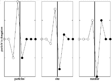
Figure 10: Schematic representation of the succession of the odd- and even- type of configurations for a DB traversing a junction from left to right. The white and black circles correspond, respectively, to particles in the A and B parts of the chain.

We refer to Fig. 10 to follow the different configurations of the DB moving from left to right through the junction. As indicated in the text, Eq. (16), we used a double perturbation expansion of the envelope function–in both $\varepsilon_{A}$ (evaluated with respect to the parameters of the A chain, see the text) and $\delta$ to compute the different configurations. Note that the convergence in $\delta$ is not as good as that for $\varepsilon_{A}$; namely, $\delta$ should be $10^{2}$ times less than $\varepsilon_{A}$ in order to get the same degree of correction for the same order of expansion in $\delta$ as in $\varepsilon_{A}$. However, the details of the calculations are lenghty and, because they present no conceptual difficulty, not given here. Instead, we give the expressions for the configurational energies of the DB in its successive appearances–as these allow us to compute the various Peierls-Nabarro barriers it encounters.

VI.2.1 Configuration I

It is of the odd-type–it corresponds to the first panel in Fig. 10: the site of maximum elongation is in part A of the chain. Its energy is found to be:

$$E_{odd}^{j(I)} = E_{odd}^{h(A)}+m_{A}\omega_{DB}^{2}\left(\frac{\alpha_{A}}{\beta_{A}}\right)\,$$ (33)

$$\times\left[\delta\left(0.13793\,\varepsilon_{A}^{-1}-0.01573+0.0056\,\varepsilon_{A}\right)\right.$$

$$\left.+\delta^{2}\left(0.49933\,\varepsilon_{A}^{-1}+0.21657-0.69346\,\varepsilon_{A}\right)\right].$$

Correspondingly, the first barrier that the DB has to overcome is the one between an even-type configuration in the homogeneous A chain and this configuration, namely:

$$E_{odd}^{j(I)}-E_{even}^{h(A)} = \Delta E_{PN}^{h(A)}+m_{A}\omega_{DB}^{2}\left(\frac{\alpha_{A}}{\beta_{A}}\right)$$ (34)

$$\times\left[\delta\left(0.13793\,\varepsilon_{A}^{-1}-0.01573+0.0056\,\varepsilon_{A}\right)\right.$$

$$\left.+\delta^{2}\left(0.49933\,\varepsilon_{A}^{-1}+0.21657-0.69346\,\varepsilon_{A}\right)\right]\,.$$

VI.2.2 Configuration II

It is of an even-type and corresponds to the second panel of Fig. 10: there are two sites with large elongations, one of them in part A of the chain, the other one in part B of the chain. The corresponding energy, up to ${\cal O}(\varepsilon_{A}^{2},\delta^{2})$, is:

$$E_{even}^{j(II)} = E_{even}^{h(A)}+m_{A}\omega_{DB}^{2}\left(\frac{\alpha_{A}}{\beta_{A}}\right)$$ (35)

$$\times\left[\delta\left(0.38117\,\varepsilon_{A}^{-1}-0.07852\right)\right.$$

$$\left.+\delta^{2}\left(-0.83444\,\varepsilon_{A}^{-1}-0.32507+1.11672\,\varepsilon_{A}\right)\right].$$

Therefore, the energy difference between configurations II and I is:

$$E_{even}^{j(II)}-E_{odd}^{j(I)} = -\Delta E_{PN}^{h(A)}+m_{A}\omega_{DB}^{2}\left(\frac{\alpha_{A}}{\beta_{A}}\right)$$ (36)

$$\times\left[\delta\left(-0.24324\,\varepsilon_{A}^{-1}-0.06280-0.00526\,\varepsilon_{A}\right)\right.$$

$$\left.+\delta^{2}\left(-1.33278\,\varepsilon_{A}^{-1}-0.54163+1.81108\,\varepsilon_{A}\right)\right]\,.$$

VI.2.3 Configuration III

Again of the odd-type, it corresponds to the third panel in Fig. 10: the site of maximum elongation is now in region B of the chain. Its energy:

$$E_{odd}^{j(III)} = E_{odd}^{h(A)}+m_{A}\omega_{DB}^{2}\left(\frac{\alpha_{A}}{\beta_{A}}\right)$$ (37)

$$\times\left[\delta\left(0.64113\,\varepsilon_{A}^{-1}-0.14880-0.00526\,\varepsilon_{A}\right)\right.$$

$$\left.+\delta^{2}\left(0.75093\,\varepsilon_{A}^{-1}+0.21657-0.68820\,\varepsilon_{A}\right)\right]\,.$$

Therefore, the energy barrier between configuration II and configuration III is:

$$E_{odd}^{j(III)}-E_{even}^{j(II)} = \Delta E_{PN}^{h(A)}+m_{A}\omega_{DB}^{2}\left(\frac{\alpha_{A}}{\beta_{A}}\right)$$ (38)

$$\times\left[\delta\left(0.25996\,\varepsilon_{A}^{-1}-0.07045-0.00526\,\varepsilon_{A}\right)\right.$$

$$\left.+\delta^{2}\left(1.58537\,\varepsilon_{A}^{-1}+0.54163-1.80493\,\varepsilon_{A}\right)\right]\,.$$

After this, the DB is essentially in the homogeneous B part [of mass $m_{B}=m_{A}(1+\delta)$]; the energies of the even- and odd-type configurations in B are:

$$E_{even}^{h(B)} = E_{even}^{h(A)}+m_{A}\omega_{DB}^{2}\left(\frac{\alpha_{A}}{\beta_{A}}\right)$$ (39)

$$\times\left[\delta\left(0.76234\,\varepsilon_{A}^{-1}-0.15705\right)\right.$$

$$\left.+\delta^{2}\left(0.38117\,\varepsilon_{A}^{-1}\right)\right]\,,$$

$$E_{odd}^{h(B)} = E_{odd}^{h(A)}+m_{A}\omega_{DB}^{2}\left(\frac{\alpha_{A}}{\beta_{A}}\right)$$ (40)

$$\times\left[\delta\left(0.77906\,\varepsilon_{A}^{-1}-0.16470\right)\right.$$

$$\left.+\delta^{2}\left(0.38953\,\varepsilon_{A}^{-1}\right)\right]\,.$$

Therefore, on one side, the energy difference between the configuration III and the even configuration of chain B is:

$$E_{even}^{h(B)}-E_{odd}^{j(II)} = -\Delta E_{PN}^{h(A)}+m_{A}\omega_{DB}^{2}\left(\frac{\alpha_{A}}{\beta_{A}}\right)$$ (41)

$$\times\left[\delta\left(0.12122\,\varepsilon_{A}^{-1}-0.00808+0.00526\,\varepsilon_{A}\right)\right.$$

$$\left.+\delta^{2}\left(-0.36976\,\varepsilon_{A}^{-1}-0.21657+0.68820\,\varepsilon_{A}\right)\right]\,,$$

and, on the other hand, the PNB in the homogeneous B part is:

$$E_{odd}^{h(B)}-E_{even}^{h(B)} = \Delta E_{PN}^{h(A)}+m_{A}\omega_{DB}^{2}\left(\frac{\alpha_{A}}{\beta_{A}}\right)$$ (42)

$$\times[\delta(0.01672\,\varepsilon_{A}^{-1}-0.00765)+\delta^{2}(0.00836\,\varepsilon_{A}^{-1})]\,.$$

VI.3 The ramp

Consider that the ramp has a “slope” $\Delta$, i.e., the mass of the $k$-th site in the ramp is

$$m_{B}(k)=m_{A}(1+k\Delta)\,\,.$$ (43)

Note that $\Delta>0$ corresponds to an up-ramp, while $\Delta<0$ to a down-ramp. Consider first a configuration of the even-type where the two sites with maximum elongation are $k-1$ and $k$. The corresponding configurational energy is found to be:

$$E_{even}^{r}(k) = E_{even}^{h(A)}+m_{A}\omega_{DB}^{2}\left(\frac{\alpha_{A}}{\beta_{A}}\right)$$ (44)

$$\times\left\{\Delta\left[(0.76234k-0.38117)\,\varepsilon_{A}^{-1}\right.\right.$$

$$\left.\left.+(-0.15705k+0.07852)\right]\right.$$

$$\left.+\Delta^{2}\left[(0.38117k^{2}-0.38117k-1.35992)\,\varepsilon_{A}^{-1}\right.\right.$$

$$\left.\left.-0.85452+3.28732\,\varepsilon_{A}\right]\right\}\,.$$

Consider then the next configurational step in the displacement of the DB from left to right on the ramp, i.e., an odd-parity type of configuration that is centered on the $k$-th site, i.e., the $k$-th site is the one that has the maximum elongation. The energy of this configuration is:

$$E_{odd}^{r}(k) = E_{odd}^{h(A)}+m_{A}\omega_{DB}^{2}\left(\frac{\alpha_{A}}{\beta_{A}}\right)$$ (45)

$$\times\left\{\Delta\left[(0.77906k+0.77906)\,\varepsilon_{A}^{-1}\right.\right.$$

$$\left.\left.-(0.16470k+0.16470)\right]\right.$$

$$\left.+\Delta^{2}\left[(0.38953k^{2}+0.77906k+2.56207)\,\varepsilon_{A}^{-1}\right.\right.$$

$$\left.\left.+0.91605-3.25850\,\varepsilon_{A}\right]\right\}\,.$$

Correspondingly, the energy barrier to overcome while moving from site $k-1$ to site $k$ is:

$$E_{odd}^{r}(k)-E_{even}^{r}(k) = \Delta E_{PN}^{h(A)}+m_{A}\omega_{DB}^{2}\left(\frac{\alpha_{A}}{\beta_{A}}\right)$$ (46)

$$\times\left\{\Delta\left[(0.01672k+1.16023)\,\varepsilon_{A}^{-1}\right.\right.$$

$$\left.\left.-(0.00765k+0.24322)\right]\right.$$

$$\left.+\Delta^{2}\left[(0.00836k^{2}+1.16023k+3.92199)\varepsilon_{A}^{-1}\right.\right.$$

$$\left.\left.+1.77057-6.54584\,\varepsilon_{A}\right]\right\}\,\,.$$

At the dominant order in both $\Delta$ and $\varepsilon_{A}$, one finds an increase in the PNB for an up mass-ramp ($\Delta>0$), and a decrease of the barrier for a down mass-ramp ($\Delta<0$).

References

- (1) S. Flach and C. R. Willis, Phys. Rep. 295, 181 (1998).
- (2) K. Hori and S. Takeno, J. Phys. Soc. Japan 61, 2186 (1992); K. Hori and S. Takeno, ibid. 4263 (1992); K. W. Sandusky, J. B. Page, and K. E. Schmidt, Phys. Rev. B 46, 6161 (1992); S. Takeno, J. Phys. Soc. Japan 61, 1433 (1992); C. Claude, Yu. Kivshar, O. Kluth, and K. H. Spatschek, Phys. Rev. B 47, 14228 (1993); T. Dauxois, M. Peyrard, and C. R. Willis, Phys. Rev. E 48, 4768 (1993); S. Flach and C. R. Willis, Phys. Rev. Lett. 72, 1777 (1994); D. Chen, S. Aubry, and G. P. Tsironis, Phys. Rev. Lett. 77, 4776 (1996); J. A. D. Wattis, Nonlinearity 9, 1583 (1996); F. M. Russell, Y. Zolotaryuk, J. C. Eilbeck, and T. Dauxois, Phys. Rev. B 55, 6304 (1997); S. Aubry and T. Cretegny, Physica D 119, 34 (1998); S. Flach, K. Kladko, Physica D 127, 61 (1999).
- (3) J. D. Kress, A. Saxena, A. R. Bishop, and R. L. Martin, Phys. Rev. B 58, 6161 (1998).
- (4) S. R. Phillpot, A. R. Bishop, and B. Horovitz, Phys. Rev. B 40, 1839 (1989).
- (5) B. I. Swanson, J. A. Brozik, S. P. Love, G. F. Strouse, A. P. Shreve, A. R. Bishop, W. Z. Wang, and M. I. Salkola, Phys. Rev. Lett. 82, 3288 (1999).
- (6) P. Binder, D. Abraimov, A. V. Ustinov, S. Flach, and Y. Zolotaryuk, Phys. Rev. Lett. 84, 745 (2000).
- (7) D. Hennig, Phys. Rev. E 62, 2846 (2000).
- (8) T. Asano, H. Nojiri, Y. Inagaki, J. P. Boucher, T. Sakon, Y. Ajiro, and M. Motokawa, Phys. Rev. Lett 84, 5880 (2000).
- (9) J. L. Marin, J. C. Eilbeck, and F. M. Russell, in Nonlinear Science at the Dawn of the 21st Century, Eds. P.L. Christiansen and M. P. Sorensen (Springer, Berlin, 2001).
- (10) F. Fillaux, C. J. Carlile, and G. J. Kearley, Phys. Rev. B 58, 11416 (1998).
- (11) See, e.g., K. Forinash, M. Peyrard, and B. Malomed, Phys. Rev. E 49, 3400 (1994); J. Cuevas, F. Palmero, and J. F. R. Archilla, arXiv:nlin/020326 and references therein.
- (12) G. P. Agrawal, Nonlinear Fiber Optics (Academic Press, Boston, 1995); S. Burtsev, D. J. Kaup, and B. A. Malomed, Phys. Rev. E 52, 4474 (1995).
- (13) T. Klinker and W. Lauterborn, Physica D 8, 249 (1983).
- (14) G. James, Comptes Rendus Acad. Sci. Serie I 332, 581 (2001).
- (15) J. B. Page, Phys. Rev. B 41, 7835 (1990).
- (16) K. W. Sandusky, J. B. Page, and K. E. Schmit, Phys. Rev. B 46, 6161 (1992); S. R. Bickham, S. A. Kiselev, and A. J. Sievers, Phys. Rev. B 47, 14206 (1993).
- (17) Note that an odd-type mode in the elongations corresponds to an even-type mode in the relative elongations, and vice-versa. In this paper, we will always refer to the modes with respect to the elongations, so that our terminology agrees with that of [Sandusky1992, ].
- (18) A. J. Sievers and S. Takeno, Phys. Rev. Lett. 61, 970 (1988).
- (19) J. L. Marín and S. Aubry, Nonlinearity 9, 1501 (1996); S. Aubry, Physica D 103, 201 (1997); J. L. Marín, S. Aubry and L. M. Floría, Physica D 113, 283 (1998).
- (20) O. M. Braun and Yu. S. Kivshar, Phys. Rev. B 43, 1060 (1991); T. Dauxois and M. Peyrard, Phys. Rev. Lett. 70, 3935 (1993); C. Claude, Yu. Kivshar, O. Kluth, and K. H. Spatschek, Phys. Rev. B 47, 14228 (1993); Yu. S. Kivshar and D. K. Campbell, Phys. Rev. E 48, 3077 (1993); T. Dauxois and M. Peyrard, Phys. Rev. E 48, 4768 (1993); S. Flach and C. R. Willis, Phys. Rev. Lett. 72, 1777 (1994); J. A. D. Wattis, Nonlinearity 9, 1583 (1996).
- (21) R. S. MacKay and J.-A. Sepulchre, Effective Hamiltonian for travelling discrete breathers, preprint, to be published in J. Phys. A: Math. Gen. (2002).
- (22) G. P. Tsironis, J. Phys. A: Math. Gen.35, 951 (2002).
- (23) D. Chen, S. Aubry, and G. P. Tsironis, Phys. Rev. Lett. 77, 4776 (1996).
- (24) R. Reigada, J. M. Sancho, M. Ibañes, and G. P. Tsironis, J. Phys. A 34, 8465 (2001); G. P. Tsironis, M. Ibañez, and J. M. Sancho, Europhys. Lett. 57, 697 (2002); M. Ibañes, J. M. Sancho, and G. P. Tsironis, Phys. Rev. E 65, 041902 (2002).
- (25) T. Dauxois and M. Peyrard, Phys. Rev. Lett. 70, 3935(1993).
- (26) Note that, as noticed also in [Sandusky1992, ], in some cases a static DB that is perturbed and starts to move stops after a certain time, it is “trapped”, although the lattice is perfectly homogeneous. In our case, this happens for very low values of the kicking coefficient. Therefore, there exists a minimum value of that has to be attained and exceeded in order to get a stable movement of the DB.
- (27) Note that an effect that is reminiscent of this one was reported in [Ibanes2002, ]. Namely, the authors considered a moving DB that traverses a curved part of a modified FPU chain (i.e., a chain with both first- and second-neighbor interactions of the FPU type). It was found that the velocity of the DB after leaving the curved region was (almost) the same, regardless of the velocity of the DB before entering the curved region. Note also that, as the authors emphasize, the same result was obtained when the “geometrical perturbation” (i.e., the presence of the curved part) of the chain was replaced by an initial random perturbation in the transverse DB direction.
- (28) Recall also that (the center of mass conservation), which leads to , . This renders such a behavior of the coefficients of the perturbative series intuitively more accessible.