Fluctuation formula and non-Gaussian distribution in the thermostated Lorentz gas

Abstract

In this paper we numerically examine the connection of the Gallavotti-Cohen fluctuation formula and the functional form of the corresponding probability density function in the field driven Lorentz gas thermostated by the Gaussian isokinetic thermostat. We analyze the moments of the entropy production rate fluctuations and show that all the central moments of the averaged fluctuations exhibit power law dependence on the length of the averaging time interval, indicating that this density deviates from a Gaussian. Furthermore the obtained exponents are found to obey a special pairing rule showing that the corresponding probability density function can not be scaled in the averaging time interval.

I Introduction

In recent years a large number of papers have focused on the Gallavotti-Cohen fluctuation formula (FF) with both theoretical and numerical tools in various nonequilibrium systems shearflow ; dynens ; onsext ; stocha ; stocha2 ; exptest ; stdystat ; maes ; flin2d ; tamas . The FF is a symmetry property of the probability density function (PDF) of a dynamically measured quantity $\xi$ connecting the probabilities of measuring $\xi$ values with equal magnitudes but opposite signs. This property was first observed numerically in a system of thermostated fluid particles undergoing shear flow shearflow where $\xi$ was the phase space contraction rate. The significance of this result was largely affected by the fact that the phase space contraction rate could be connected to the entropy production rate, thus the FF gave an insight to the nonequilibrium thermodynamical behavior of the system. Since then the nontrivial connection of the phase space contraction rate and the entropy production rate has been investigated and was treated in epr .

More precisely, let $\xi_{\tau}(t)$ denote the quantity $\xi$ averaged over a time interval of length $\tau$ centered around time $t$: $\xi_{\tau}(t)=\frac{1}{\tau}\int\limits_{-{\tau}/{2}}^{{\tau}/{2}}\xi(t+t^{\prime})\,\mathrm{d}t^{\prime}$. Considering it as a stochastic variable, its statistical properties in a steady state can be characterized by a probability density function $\Xi_{\tau}(x)$. The FF states that this PDF has the following property:

$$\lim_{\tau\to\infty}\frac{1}{\tau}\ln\frac{\Xi_{\tau}(x)}{\Xi_{\tau}(-x)}=x\,.$$ (1)

In other words, the probability of observing a negative $\xi$ value is exponentially smaller than that of the corresponding positive value in the $\tau\to\infty$ limit.

The FF has also been found to be valid in certain systems with strong external forcing chaodyn , thus it is expected to say something important about systems far from equilibrium (as opposed to linear response theory, which is valid for vanishing external fields). Consequently, significant theoretical efforts have been made to find a common property behind this behavior in all the systems obeying the FF dynens ; stocha ; stocha2 ; maes .

Since the FF connects the values of the $\Xi_{\tau}(x)$ function on the negative half axis to the values of $\Xi_{\tau}(x)$ on the positive one, but it does not state anything about the functional form of $\Xi_{\tau}(x)$, it is interesting to examine the latter in systems found to obey the FF. This question is emphasized by the observation that Eq. (1) can be satisfied by a Gaussian PDF with a subcondition connecting its average and variance. This raises the necessity to study how close the underlying PDF of $\Xi_{\tau}(x)$ is to a Gaussian in systems which seem to obey the FF.

In a previous paper flform we investigated numerically the validity of the FF in the two and three dimensional periodic LG subject to a constant electric and magnetic field and thermostated by the GIK thermostat. We found that the symmetry property described by the FF is valid for low and high $\tau$ values in the reversible configurations and seems to be approximately valid in the $\tau\to\infty$ limit even in the absence of reversibility. This also motivated us to study the $\tau$-dependence of the details of $\Xi_{\tau}(x)$ in the thermostated LG.

In this paper we numerically analyze the connection of obeying the FF and the details of the functional form of the corresponding PDF in the periodic Lorentz Gas (LG) thermostated by a Gaussian Isokinetic (GIK) thermostat. In Sec. II we describe the simulated system, in Sec. III we present our numerical results and in Sec. IV we summarize our conclusions.

II The system

One of the simplest and most investigated models suitable for studying transport phenomena is the field driven Lorentz gas (LG) thermostated by a Gaussian isokinetic (GIK) thermostat. This model consists of a charged particle subjected to an electric field moving in the lattice of elastic scatterers. Due to the applied electric field, one must use a thermostating mechanism to achieve a steady state in the system. Such a tool is the Gaussian isokinetic thermostat which preserves the kinetic energy of the particle thermostats .

For the sake of simplicity, we investigate in our study the two dimensional (2D) periodic Lorentz gas with circular scatterers arranged on a square lattice. We present the equations of motion in dimensionless variables: choosing the unit of mass $m$ and electric charge $q$ to be equal to the mass and electric charge of the particle, yields $m=q=1$ in our model. The unit of distance is taken to be equal to the radius of scatterers ($R=1$), and the unit of time is chosen to normalize the magnitude of particle velocity to unity. Let ${\bf q}=\left(q_{1},q_{2}\right)$ denote the position and ${\bf p}=\left(p_{1},p_{2}\right)$ the momentum of the particle ($\left|{\bf p}\right|=1$). The phase space variable of the system is ${\mathbf{\Gamma}}=\left({\bf q},{\bf p}\right)$; it is transformed abruptly at every elastic collision and evolved smoothly by the differential equation

$$\dot{\bf q} = {\bf p}$$

$$\dot{\bf p} = {\bf E}-\alpha{\bf p}$$ (2)

between the collisions. Here $\alpha$ is called the thermostat variable, while ${\bf E}$ is the constant vector playing the role of the external electric field. The GIK thermostat requires the fixing of the kinetic energy, which leads to the choice $\alpha={\bf E}{\bf p}$ in Eq. (II).

Dissipation in such models can be measured by the phase space contraction rate $\sigma$. It can be computed by taking the divergence of the right-hand side of Eq. (II):

$$\sigma=-\mbox{div}\,{\bf\dot{\Gamma}}=\alpha\,,$$ (3)

and it can be shown that in this model

$$\sigma(t) = \xi(t),$$ (4)

where $\xi$ is the entropy production rate defined according to the $\xi=\frac{\bf JE}{k_{B}T}$ expression of irreversible thermodynamics, and the temperature $T$ is given by analogy with kinetic theory epr . We note that while Eq. (4) is valid for the GIK thermostat, it need not be true in general, as shown e.g. in models thermostated by some variants of the Nosé-Hoover thermostat nosehoover or by deterministic scatterings detscatt .

III Numerical results

The goal of our numerical simulations is to measure $\Xi_{\tau}(x)$ with a precision that is sufficient to check the validity of the fluctuation formula, as well as the question of Gaussianity of the distribution. Due to Eq. (4), $\Xi_{\tau}(x)$ can be measured by periodically computing $\xi_{\tau}$ along a long particle trajectory and making a histogram of these data. The disadvantage of this method is that the range of possible $\xi_{\tau}$ values depends on the strength of the electric field. Instead of $\xi_{\tau}$, we may introduce the quantity

$$\pi_{\tau}(t)=\frac{1}{\tau}\int\limits_{-\frac{\tau}{2}}^{\frac{\tau}{2}}{\bf n_{E}}{\bf p}(t+t^{{}^{\prime}})\,\mathrm{d}t^{{}^{\prime}},$$ (5)

where ${\bf n_{E}}$ denotes the unit vector parallel to ${\bf E}$. Since the magnitude of ${\bf p}$ is unity, $\pi_{\tau}$ always satisfies $\pi_{\tau}\in[-1,1]$. By making a histogram of the periodically measured values of $\pi_{\tau}$, one gets an approximation of its probability density $\Pi_{\tau}(x)$ shown in Fig. 1.

Figure 1: The probability density $\Pi_{\tau}(x)$ in the 2D periodic LG, with lattice constant $d=2.1$ and external field ${\bf E}=(0.3,0.48)$, the number of collisions is $1.58\times 10^{7}$ and the averaged time between two collisions is $\approx 0.62$. For higher $\tau$ values the curves seems to be “Gaussian like”: fitting a Gaussian function onto the measured values yields very good visual agreement.

The two stochastic variables defined above satisfy $\xi_{\tau}=E\pi_{\tau}$, so the relationship between two probability densities $\Xi_{\tau}$ and $\Pi_{\tau}$ is simply $\Xi_{\tau}(x)=\frac{1}{E}\,\Pi_{\tau}\left(\frac{x}{E}\right).$

III.1 Scaling

We can observe in Fig. 1 that for high enough $\tau$ values the PDF $\Pi_{\tau}(x)$ seems to be close to a Gaussian. In order to examine this behavior we applied the following scaling transformation to the $\Pi_{\tau}(x)$ functions:

$$S_{\tau}(x)=\frac{1}{\Pi^{\left(max\right)}_{\tau}}\Pi_{\tau}\left(\frac{x}{\Pi^{\left(max\right)}_{\tau}}+x_{max}\right).$$ (6)

In this equation $x_{max}$ denotes the $x$-value where $\Pi_{\tau}(x)$ takes its maximal value denoted by $\Pi^{\left(max\right)}_{\tau}$.

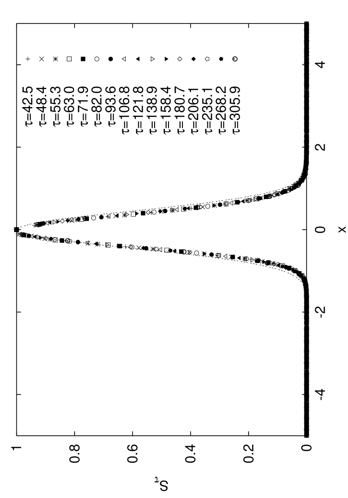
Figure 2: The $S_{\tau}(x)$ scaled function of $\Pi_{\tau}(x)$ for different $\tau$ values with field ${\bf E}=(0.3,0.48)$ (the same configuration as for Fig. 1). The dashed curve shows the Gaussian function $S_{G}(x)=e^{-\sqrt{2\pi}x^{2}}$.

Observing in Fig. 3 that the standard deviation of $\Pi_{\tau}(x)$ is proportional to $1/{\sqrt{\tau}}$ (thus $\Pi^{\left(max\right)}_{\tau}\sim\sqrt{\tau}$), one can see that Fig. 2 shows $\pi_{\tau}$ fluctuations of $O(1/{\sqrt{\tau}})$. It is worth noting that fluctuations of this magnitude also constitute the range where the central limit theorem (CLT) could in principle guarantee the Gaussian form of $S_{\tau}(x)$ for high enough $\tau$ values. Indeed, by examining Fig. 2 we can conclude that for high $\tau$ values all the measured points of $S_{\tau}(x)$ are close to the Gaussian $S_{G}(x)=e^{-\sqrt{2\pi}x^{2}}$.

III.2 The moments

In order to characterize the deviation of the PDF from a Gaussian, we compute its moments and cumulants from the simulated distribution. Let $m^{(i)}$, $c^{(i)}$ and $q^{(i)}$ denote the $i$’th order moment, central moment and cumulant of $\Pi_{\tau}(x)$ respectively ($i=1,2,3,\ldots$) moments . First we deal with the central moments of $\Pi_{\tau}(x)$ for a given configuration of the periodic LG, shown in Fig. 3. Based on this figure, we can make several important observations.

1. The central moments of order $i$ $c^{(i)}_{\tau}$ exhibit power law dependence on $\tau$ with exponents $\beta_{i}$ depending on $i$: $c^{(i)}_{\tau}\approx\alpha_{i}\tau^{-\beta_{i}}$; Table (1) lists the numerical values of $\alpha_{i}$ and $\beta_{i}$ found in the simulation.

2. The exponents $\beta_{i}$ are found to form pairs, at least approximately: $\beta_{3}\approx\beta_{4}$, $\beta_{5}\approx\beta_{6}$, and so on.

3. The even order central moments behave the same way as for a Gaussian distribution, i.e., they all can be computed from the variance alone. The Gaussian moments $c_{G}^{(i)}$ calculated in this way from $c^{(2)}$ are shown as continuous lines in the figure, and indeed, they seem to run very close to the actual measured values of the even order central moments.

Analyzing several configurations with various strengths and directions of the external field, we found that the $\beta_{i}$ exponents are approximately the same in all the configurations. In contrast, the $\alpha_{i}$ factors do depend on the details of the chosen configuration.

Figure 3: The central moments $c^{(i)}_{\tau}$ of $\Pi_{\tau}(x)$ in the 2D periodic LG. In this configuration ${\bf E}=(0.3,0.48)$, the collision number is $1.5\times 10^{7}$. The continuous lines show the behavior expected from Gaussian moments: $c^{(4)}_{G}=3\,{c^{(2)}}^{2}$, $c^{(6)}_{G}=15\,{c^{(2)}}^{3}$, $c^{(8)}_{G}=105\,{c^{(2)}}^{4}$, $c^{(10)}_{G}=945\,{c^{(2)}}^{5}$, etc., calculated from $c^{(2)}$.

$i$	$\beta_{i}$	$\alpha_{i}$
$2$	$0.961\pm 0.003\approx 1$	$0.224\pm 0.003$
$3$	$2.047\pm 0.016\approx 2$	$0.225\pm 0.017$
$4$	$1.965\pm 0.005\approx 2$	$0.190\pm 0.005$
$5$	$3.046\pm 0.048\approx 3$	$0.614\pm 0.048$
$6$	$3.005\pm 0.004\approx 3$	$0.330\pm 0.007$
$7$	$4.023\pm 0.024\approx 4$	$1.616\pm 0.181$
$8$	$4.052\pm 0.005\approx 4$	$0.868\pm 0.021$
$9$	$4.937\pm 0.038\approx 5$	$3.742\pm 0.656$
$10$	$5.068\pm 0.187\approx 5$	$2.631\pm 0.187$

Table 1: The exponent $\beta_{i}$ and the prefactor $\alpha_{i}$ of the $i$-th central moment shown on Fig. 3. These values are computed using the NLLS Marquardt-Levenberg algorithm included in gnuplot to fit the measured data points with a power function on the interval $[100,1000]$. The errors presented here come from the fitting method. The odd order moments seem to run close to their even successors: $\beta_{2n+1}\approx\beta_{2(n+1)}\approx n+1$.

Now we compare our findings to the expectations based on a Gaussianity assumption. Because of the power law dependence in the odd order central moments, we can say that $\Pi_{\tau}(x)$ is definitely not Gaussian for any finite value of $\tau$ (they all should be zero for a Gaussian distribution). On the other hand, the distributions $\Pi_{\tau}(x)$ do seem to converge to a Gaussian in the limit $\tau\to\infty$. This can be checked in Fig. 4 showing the behavior of the cumulants: all of the higher ($i>2$) order cumulants go to zero faster than those of order $i=1,2$ in the $\tau\to\infty$ limit.

Figure 4: The absolute values of the cumulants $q_{\tau}^{(i)}$ of $\Pi_{\tau}(x)$ in the periodic LG. The configuration is the same as for Fig. 3. $\Pi_{\tau}(x)$ converges to a Gaussian in the $\tau\to\infty$ limit. Since $q^{(3)}\sim\tau^{-2}$, the convergence of $\Pi_{\tau}(x)$ to a Gaussian is power like; the deviation is on the order of $\tau^{-2}$.

Another important consequence of the pairing of the $\beta_{i}$ exponents is that $\Pi_{\tau}(x)$ can not be scaled in the sense of Eq. (6). Indeed, the equation $S_{\tau}(x)=S(x)$ results that $\Pi_{\tau}\left(x+m\right)=\Pi^{\left(max\right)}_{\tau}S\left(\Pi^{\left(max\right)}_{\tau}x\right)$, since $x_{max}=m$ for high $\tau$ values. Substituting this equation into the definition of the central moments and performing the variable transformation $y=\Pi^{\left(max\right)}_{\tau}x$ yields

$$c_{i}=\int_{-\infty}^{\infty}\,\mathrm{d}x\Pi_{\tau}(x+m)x^{i}=$$

$$\int_{-\infty}^{\infty}\,\mathrm{d}x\Pi^{\left(max\right)}_{\tau}S\left(\Pi^{\left(max\right)}_{\tau}x\right)x^{i}=$$ (7)

$$\left(\Pi^{\left(max\right)}_{\tau}\right)^{-i}\int_{-\infty}^{\infty}\,\mathrm{d}yS(y)y^{i}\,.$$

The last expression shows that if $S_{\tau}(x)=S(x)$ were true in this system, then the $\beta_{i}$ exponents should obey the $\beta_{i}=\frac{i}{2}$ identity, since $\Pi^{\left(max\right)}_{\tau}\sim\sqrt{\tau}$ for high $\tau$ values. Table 1 shows that the odd order $\beta_{i}$ exponents deviate significantly from $\frac{i}{2}$. This behavior indicates that the scaling property suggested by Fig. 2 can only be treated as a good approximation and not as an exact result in the GIK thermostated LG. This also raises the question whether similar claims of scaling, based on the visual properties of the PDF in other systems as e.g. in Ref. observ , could also be supported by the behavior of the moments.

III.3 The Fluctuation Formula

We can rewrite the FF in the terms of $\Pi_{\tau}(x)$ as

$$\lim_{\tau\to\infty}\frac{1}{E}\frac{1}{\tau}\,\ln\frac{\Pi_{\tau}(x)}{\Pi_{\tau}(-x)}=x\,.$$ (8)

In order to visualize the FF, we introduce the quantity

$$D_{\tau}(x)=\frac{1}{E}\frac{1}{\tau}\,\ln\frac{\Pi_{\tau}(x)}{\Pi_{\tau}(-x)}.$$ (9)

If the FF is satisfied in the system, then $D_{\tau}(x)$ is linear with slope 1 in the $\tau\to\infty$ limit. Analyzing the behavior of this quantity in Fig. 5 one can make two important observations:

1. The FF is satisfied quite well for both low $\tau$ values and for large ones (in this context, low $\tau$ value means 6-8 times the average time between two subsequent collisions).

2. As $\tau$ gets higher, the interval where $D_{\tau}(x)$ can be plotted is getting narrower and narrower. This is a consequence of the fact that for higher $\tau$ values large fluctuations of $\xi_{\tau}$ become less and less probable. In other words fluctuations outside the plotted range are practically unobservable.

We note that we tested several other configurations with various choices of the magnitude and direction of the electric field ${\bf E}$ in the ergodic range ergodic , and we didn’t find any relevant deviation from the behavior presented above.

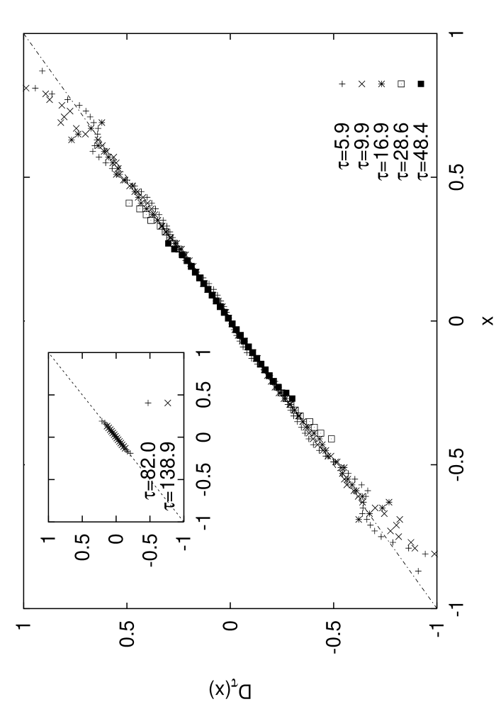
Figure 5: $D_{\tau}(x)$ in the same configuration as for Fig. 1. The inset shows $D_{\tau}(x)$ for higher $\tau$ values. The inset and the figure have the same axes.

III.4 The Gaussian approximation

Since we have seen that the even order central moments behave in a Gaussian way, it is worth checking if the subcondition that leads to the FF for Gaussian distributions holds for $\Pi_{\tau}(x)$. This subcondition can be derived by substituting $\Pi_{\tau}(x)=\frac{1}{\sqrt{2\pi}\sigma_{\tau}}\exp{\left(\frac{-(x-m_{\tau})^{2}}{2\sigma_{\tau}^{2}}\right)}$ into Eq. (8). This leads to the following formula:

$$\lim_{\tau\to\infty}\frac{1}{E}\frac{1}{\tau}\frac{2m_{\tau}}{\sigma_{\tau}^{2}}=1\,,$$ (10)

where $m_{\tau}=m^{(1)}_{\tau}$ and $\sigma_{\tau}^{2}=c^{(2)}_{\tau}$ according to the previous notation.

In Fig. 6 we can verify that the $\frac{1}{E}\frac{1}{\tau}\frac{2m_{\tau}}{\sigma_{\tau}^{2}}=1$ identity is violated for all finite $\tau$ values but satisfied in the $\tau\to\infty$ limit. On the other hand, we have seen in Fig. 5 that the FF is valid with reasonable precision even for low values of $\tau$. These observations indicate that:

1. For finite $\tau$ values the the odd order moments also contribute to the fulfillment of the FF, thus the Gaussian approximation of the PDF $\Pi_{\tau}(x)$ violates the FF. This behavior is also supported by the analysis performed in Ref. exptest .

2. For high $\tau$ values the observable part of the PDF $\Pi_{\tau}(x)$ seems to converge to a Gaussian (see. Fig. 2) and the Gaussian approximation of the PDF $\Pi_{\tau}(x)$ satisfies the FF.

Figure 6: The quantity $\frac{1}{E}\frac{1}{\tau}\frac{2m_{\tau}}{\sigma_{\tau}^{2}}$ at different field strengths ${\bf E}$ in the 2D periodic Lorentz Gas. In these configurations ${\bf E}$ is parallel with $(0.3,0.48)$ and the collision number is $\approx 1.5\times 10^{7}$. The curves deviate from 1 for all the $\tau$ values presented on the figure, however seem to converge to 1 in the $\tau\to\infty$ limit.

This is in agreement with the observed behavior of the cumulants indicating a convergence to Gaussian distributions for $\tau\to\infty$; indeed, for Gaussian distributions the FF is equivalent to Eq. (10).

Figure 7: The dependence of $\Delta_{\tau,E}$ on $\tau$ for different field strengths. The direction of ${\bf E}$ is parallel with $(5,8)$ but its magnitude varies. The curves appear to be linear in the dominant region on the log-log plot, suggesting a power law dependence on $\tau$.

III.5 The observability of large fluctuations

Since we have shown that for high $\tau$ values neither $\Pi_{\tau}(x)$ nor $D_{\tau}(x)$ can be observed on the whole interval $[-1,1]$, we introduce $\Delta_{\tau,E}$ to quantify where $D_{\tau}(x)$ can be observed, i.e. where the FF can be tested. Let $[-\Delta_{\tau,E},\Delta_{\tau,E}]$ denote the interval where $D_{\tau}(x)$ can be reconstructed from a given time series in a specific configuration. Data from our numerical simulations are summarized in Fig. 7. It shows that $\Delta_{\tau,E}$ has a power-law dependence on $\tau$:

$$\Delta_{\tau,E}\sim\tau^{-\delta(E)}\,,$$ (11)

where the exponent $\delta$ tends to increase with increasing field strengths.

IV Conclusion

In this paper we have investigated numerically the PDF of the EPR fluctuations for both low and high averaging time intervals in the 2D periodic LG thermostated by the GIK thermostat. We have shown that for low averaging time intervals the EPR fluctuations are definitely not Gaussian, but they satisfy the Gallavotti-Cohen fluctuation formula. For high averaging time intervals the EPR fluctuations are converging to a Gaussian distribution and still obeying the FF, thus the Gaussian approximation of the EPR fluctuations seems to be better and better as $\tau$ gets higher in this model. We have analyzed the moments of the corresponding PDF to characterize its functional form and found a special power-law dependence (pairing of the $\beta_{i}$ exponents) of the central moments on the averaging time interval. Our results raise the question whether the $\beta_{i}$-pairing could be observed in other systems satisfying the FF, or this is just a special property of the GIK thermostated Lorentz gas.

- (1) D.J. Evans, E.G.D. Cohen and G.P. Morriss, Phys. Rev. Lett. 71, 2401 (1993)
- (2) G. Gallavotti and E.G.D. Cohen, Phys. Rev. Lett. 74, 2694 (1995)
- (3) G. Gallavotti, Phys. Rev. Lett. 77, 4334 (1996)
- (4) J. Kurchan, J. Phys. A, 31, 3719 (1998)
- (5) D.J. Searles and D.J. Evans, Phys. Rev. E 60, 159 (1999)
- (6) F. Bonetto, G. Gallavotti and P.L. Garrido, Physica 105D, 226 (1997)
- (7) D.J. Evans and D.J. Searles, Phys. Rev. E 52, 5839 (1995)
- (8) C. Maes, J. Stat. Phys, 95, 367 (1999)
- (9) L. Rondoni and E. Segre, preprint eprint chao-dyn/9810028
- (10) L. Rondoni, T. Tél and J. Vollmer, Phys. Rev. E 61, 4679 (2000)
- (11) See e.g. E.G.D. Cohen and L. Rondoni, Chaos 8, 357 (1998)
- (12) For an overview, see G. Gallavotti, Chaos 8, 384 (1998) and references therein.
- (13) M. Dolowschiák and Z. Kovács, Phys. Rev. E 66, 066217 (2002)
- (14) For a review of deterministic thermostats, see G.P. Morriss and C.P. Dettmann, Chaos 8, 321 (1998) and references therein.
- (15) K. Rateitschak, R. Klages and W.G. Hoover, J. Stat. Phys. 101, 61-77 (2000)
- (16) K. Rateitschak and R. Klages, Phys. Rev. E 65, 036209 (2002)
- (17) Obviously the quantity in question is , however it is easier to work with . The connection between the analogous quantities of the two PDFs and can easily be derived. Let , and denote the ’th order moment, central moment and cumulant pertaining to , then: , and .
- (18) L. Rondoni and G.P. Morriss, Preprint ESI 1148 (Vienna, 2002)
- (19) The dynamics of the periodic LG thermostated by a GIK thermostat is nonergodic for high external fields, as shown first in J.Lloyd, L.Rondoni and G.P.Morriss, Phys. Rev. E 50, 3416 (1983). Since we have used a different lattice (cubic) in our numerical study, we checked the ergodicity of our model for different field values and found behaviors similar to the ones reported in that paper: for low values the dynamics seems to be ergodic, but for high values () the breakdown of ergodicity can be observed.