Resonance-Assisted Tunneling

Abstract

We present evidence that tunneling processes in near-integrable systems are enhanced due to the manifestation of nonlinear resonances and their respective island chains in phase space. A semiclassical description of this “resonance-assisted” mechanism is given, which is based on a local perturbative description of the dynamics in the vicinity of the resonances. As underlying picture, we obtain that the quantum state is coupled, via a succession of classically forbidden transitions across nonlinear resonances, to high excitations within the well, from where tunneling occurs with a rather large rate. The connection between this description and the complex classical structure of the underlying integrable dynamics is furthermore studied, giving ground to the general coherence of the description as well as guidelines for the identification of the dominant tunneling paths. The validity of this mechanism is demonstrated within the kicked Harper model, where good agreement between quantum and semiclassical (resonance-assisted) tunneling rates is found.

PACS: 05.45.Mt, 03.65.Sq, 03.65.Xp

I Introduction

Since the early days of quantum mechanics, tunneling has been recognized as one of the hallmarks of the wave character of microscopic physics. The possibility of a quantum particle to penetrate an energetic barrier – or, more generally, a dynamical barrier in phase space, as termed by “dynamical tunneling” [1] – represents certainly one of the most spectacular implications of quantum theory and has lead to various applications in atomic and molecular physics as well as in mesoscopic science (for instance in the context of spintronics devices [2] to mention just one recent example). Despite its genuinely quantal nature, however, tunneling is strongly influenced, if not entirely governed by the structure of the underlying classical phase space. Tuning the classical dynamics from an integrable to a chaotic one substantially modifies the tunnel coupling - not only if the chaos affects the classically allowed motion (a case that was studied in detail in [3]), but also if the destruction of invariant tori is restricted to phase space domains deep inside the classically forbidden regions.

Tunneling processes take place in a variety of contexts. One may for instance be interested in the coupling of a metastable state to a continuum, as, e.g., in the case of the $\alpha$-particle decay. The tunneling process manifests then in form of a finite life time of the state, or equivalently, in a finite width of the corresponding spectral resonance. Another situation concerns systems that possess a discrete symmetry $P$, in such a way that Rabi oscillations can take place between states that are localized in symmetric regions of the phase space. The effectiveness of tunneling is then related to the period of the Rabi oscillations, or equivalently to the splittings between the corresponding symmetric and antisymmetric eigenmodes.

Here, for the sake of definiteness, we shall restrict ourself to this latter configuration, though our study could be applied with minor modification to other contexts such as the computation of resonance widths. To be more specific, we shall consider systems the classical dynamics of which exhibits, due to the discrete symmetry, two congruent but separate regions of regular, bound motion in phase space. Semiclassical Einstein-Brillouin-Keller (EBK) quantization then provides a prescription how to construct local eigenmodes on quantized tori within each of the regions. These “quasimodes” fulfill the Schrödinger equation, possibly to all powers in $\hbar$, but do not take into account the behavior of the wavefunction in the forbidden domain, and are therefore characterized by equal energies for any pair of symmetry related quantized tori. It is the nonclassical coupling between the quasimodes that lifts this degeneracy and selects the symmetric and the antisymmetric linear combination of these states as true eigenstates of the quantum system. Provided the classical dynamics is integrable, the tunnel coupling that produces this level splitting can be reproduced by the analytic continuation of the torus structure into complex domain. In case of a one-dimensional motion generated by the usual $p^{2}/2+V(x)$ Hamiltonian, this amounts to calculating an imaginary action integral of the type $\int\sqrt{2(V(x)-E)}dx$ in between the two wells.

Such a dynamical tunneling process also takes place in nonintegrable systems, but with substantially different effectiveness. By applying a nonintegrable perturbation on the dynamics in such a way that an appreciable chaotic layer is introduced in between the two regular regions, the tunnel coupling between the quasimodes is significantly enhanced with respect to the integrable system [4, 5, 6]. Moreover, the tunneling rates do no longer exhibit a well-defined scaling with Planck’s constant (which would be an exponential decrease with $1/\hbar$ in an integrable system), but may undergo huge quasierratic fluctuations for small variations of $\hbar$ [4, 5, 6].

These phenomena are traced back to the specific role that chaotic states play in such systems [5, 6, 7] In contrast to integrable dynamics, the tunnel doublets of the localized quasimodes are in a mixed system no longer isolated in the spectrum, but resonantly interact with states that are associated with the chaotic part of phase space. Due to their delocalized nature, such chaotic states typically exhibit a considerable overlap with the boundary regions of both regular wells. They may therefore provide an efficient coupling mechanism between the quasimodes – which becomes particularly effective at values of $\hbar$ (or any other external parameter) at which one of the chaotic level is shifted exactly on resonance with the tunnel doublet. This interpretation was basically confirmed by a statistical analysis of the fluctuations of the level splittings, which were shown to be in good agreement with the corresponding prediction that a random matrix model of the chaotic part of phase space would yield [6, 8]. Evidence for chaos-assisted tunneling was found in theoretical calculations of the life times of nondispersive wave packets in microwave driven hydrogen [9] and, most recently, also in experiments on ultracold atoms that were stored within periodically modulated optical lattices [10, 11, 12]. Also for electromagnetic systems, in particular within microwave billiards [13] and optical microcavities [14], it was verified that (ray optical) chaos has a strong impact on wave tunneling.

Apart from this qualitative insight and its quantitative statistical modeling, however, little is known about chaos-assisted tunneling from the semiclassical point of view. In particular, there exists no practicable semiclassical tool up to now for estimating the tunnel coupling from a torus within a regular island to the chaotic sea (which would provide valuable information about the magnitude around which the tunnel rates fluctuate). This is essentially due to the fact that in nonintegrable systems invariant tori are generally characterized by a restricted domain of analyticity and can therefore not be continued far enough into the complex domain to reproduce the tunnel coupling [15, 16]. As has been shown by Shudo and coworkers [17], it is in principle possible to semiclassically reconstruct the tunneling tail of the time evolution of some initial wavefunctions within a mixed system by summing up the contributions of all complex classical trajectories that fulfill appropriate boundary conditions. This requires the analysis of a highly complicated manifold of initial conditions in complex phase space, where the Stokes phenomenon plays a crucial role for the selection of contributing trajectories [17]. Though successful from the quantitative point of view, this method is limited to initial values problems, and it is not evident how much insight it may provide for an intuitive understanding of the properties of eigenfunctions.

The present contribution can in some sense be seen as a complementary approach with respect to the work of Shudo et al. [17]. We shall, however, not tackle directly mixed regular-chaotic dynamics, but consider a conceptually simpler situation, namely the nearly integrable regime in which chaos is not yet fully developed. In this context, it has been pointed out by Bonci and co-workers [18] that classical resonances should play a crucial role in such systems. As nonlinear resonances between two classical eigenmodes arise whenever their frequencies are related by a rational multiple, they generally lead to quasi-degeneracies of the associated levels in the spectrum. This may therefore induce significant couplings to higher states within the regular region, from which tunneling occurs with a much faster rate than from the original state. Besides the aspect of near-degeneracies – which alone is not sufficient for a quantitative understanding of the role of resonances, as level crossings arise also in integrable systems without introducing any modification – it is also important to take into account the magnitude of the effective matrix element that couples the near-degenerate states. This quantity is directly related to the structure of the underlying classical phase space. Within the action-angle variable representation of the unperturbed integrable dynamics, a nonlinear resonance generally manifests in form of a pendulum-like perturbation, and the associated modification of the torus structure in its vicinity is then responsible for couplings across the resonance, the strength of the coupling being determined by the extension of the pendulum structure in phase space [19, 20, 21, 22].

Our previous publication [23] has shown that the combination of these two aspects, namely the near-degeneracy and the coupling induced by the resonance, form the basis of a mechanism that governs tunneling in the near-integrable limit. This study was performed within the “kicked Harper” model, a one dimensional time periodic system governed by the Hamiltonian

$$H(p,q,t)=\cos p+\tau\sum_{n=-\infty}^{\infty}\delta(t-n\tau)\cos q$$ (1)

the dynamics of which is equivalent to the symplectic map

$$p^{\prime} = p+\tau\sin{q}$$ (2)

$$q^{\prime} = q-\tau\sin{p^{\prime}}\;$$ (3)

which describes how the phase space variables $(p,q)$ evolve from time $t=n\tau$ (more precisely, from the time immediately before the kick) to time $t=(n+1)\tau$. This model has proven its usefulness in the context of many different aspects related to quantum chaos [24, 25, 26] (including also dynamical tunneling [27]). Our study was restricted to a relatively small value $\tau=1$ of the perturbation parameter, for which the classical dynamics in nearly integrable. The quantum tunneling rates that are obtained at this perturbation strength are shown in Fig.1. We see that, despite a seemingly “regular” phase space (shown in Fig. 2), they are nontrivial and exhibit similar features as in the case of a truly mixed regular-chaotic system: Even for rather small deviations from integrability, the tunneling rates may, in the semiclassical regime, become appreciably enhanced with respect to the integrable limit (by a factor that may reach up to ten orders of magnitude in the case that we have considered in [23]) and do not follow a monotonous exponential scaling with $1/\hbar$.

As key ingredient to understand such a behavior, we have introduced an integrable approximation of the kicked Harper map (in an analogous way as in [28]) which, even in the case of moderate perturbations, provides a reasonable description of the nearly integrable motion on the invariant tori. Expanding the kicked Harper eigenfunctions within the eigenbasis of this integrable approximation allowed to unambiguously identify resonances as the source of modifications in the tunneling tail of the eigenfunctions. A quantitative reproduction of the tunneling rates in the kicked Harper, the accuracy of which is visible on Fig. 1, was then achieved through a quantum perturbative treatment of a local effective Hamiltonian, which is formally derived via secular perturbation theory of the classical motion [29] and was in practice obtained via the Fourier analysis of the separatrix structure associated with the resonance [23].

The combination of these “tools” has evidently proven successful for the identification of the underlying mechanism as well as for a low-cost (with respect to computer memory) calculation of tunnel splittings that would otherwise be accessible only through a full quantum treatment of the problem. However, the justification of the resonance-assisted mechanism presented in [23] was mainly based on the demonstration of its quantitative predictive power for reasonably small values of $\hbar$ within the kicked Harper system. In this paper, we would like to go further in the understanding of the tunneling process in the nearly integrable regime. A central question that we shall address is to which extent the resonance-assisted tunneling mechanism we propose should in general be the dominant one, and what modifications are to be expected as the system is pushed deep in the semiclassical regime. A general issue that underlies these interrogations is the fact that the approach we propose is based on a combination of perturbative techniques (both classical and quantum) and semiclassical concepts, and therefore involves essentially two small parameters: the perturbation strength which enters in a purely algebraic way into the coupling terms, and the quantum coarse graining $\hbar$ on which these terms depend both algebraically and exponentially. Although we obviously do not intend to attain anything like mathematical rigor, our goal in this paper is to give evidence that the global picture that underlies resonance-assisted tunneling “makes sense” and, on a more practical tone, may lead to guiding rules for the identification of dominating terms in the tunneling mechanism.

To reach this objective, we shall see that it is useful to provide a more geometric vision of resonance-assisted tunneling. This means on the one hand that we shall emphasize the connection between the coefficients that describe the strength of the coupling and the complex structure of the underlying integrable approximation. On the other hand, we shall see how the coupling via a nonlinear resonance can be considered as dynamical tunneling process, in very much the same spirit as the coupling between quasimodes on symmetry-related invariant tori. However, the effective topology of complex tori that the quantum system encounters in order to undergo the tunneling transition sensitively depends on the quantum coarse graining. For rather large $\hbar$, a direct connection between the quasidegenerate tori of the two wells is “seen” by the quantum system. Deeper in the semiclassical regime, the tori rather appear as being connected, via one or several resonances, to higher excitations within the well, from where a transition across the separatrix is associated with a rather low imaginary action.

Our study will be restricted to one-degree-of-freedom systems subject to a time-periodic perturbation with period $\tau$ or frequency $\omega=2\pi/\tau$. We denote by $\hat{H}(\hat{p},\hat{q},t)=\hat{H}(\hat{p},\hat{q},t+\tau)$ the quantum Hamiltonian and by $H(p,q,t)$ its classical limit. The classical phase is most conveniently visualized by means of a Poincaré surface of section in time domain – i.e., by the area-preserving map

$${\mathcal{T}}:(p_{t},q_{t})\longmapsto(p_{t+\tau},q_{t+\tau})$$ (4)

that describes the evolution of the phase space variables $(p,q)$ from time $t$ to time $t+\tau$. Quantum mechanically we shall, in analogy, consider the quantum propagator

$$\hat{U}=\exp\left(\frac{i}{\hbar}\int_{0}^{\tau}\hat{H}(t)dt\right)\;,$$ (5)

and study its eigenfunctions $|\psi_{k}\rangle$ and eigenphases $\phi_{k}$, defined by

$$\hat{U}|\psi_{k}\rangle=e^{i\phi_{k}}|\psi_{k}\rangle\;.$$ (6)

Whenever an illustrative example appears appropriate, we shall make use of the kicked Harper Hamiltonian [24] Eq. (1) the Poincaré map of which is given by Eq. (3). We shall, however, try to keep the discussion as general as possible in order to allow an application also to other time-periodic tunneling problems such as the driven double well [4, 30] or the effective Hamiltonian [12] that was employed in the context of the recent dynamical tunneling experiments in cold atoms [10, 11].

To lay firm foundations, we begin in Sec. II with a brief review of what we like to name “regular tunneling” – i.e., the attempt to semiclassically describe tunneling by a direct analytic continuation of the invariant tori into the complex phase space. We shall argue, however, that this concept is, strictly speaking, limited to exactly integrable systems and breaks down when a small nonintegrable perturbation is applied. This naturally leads to the question of how nonlinear resonances influence tunneling, which we shall discuss in Sec. III. We shall begin, in Sec. III A, with a formal description of the classical dynamics in the vicinity of a nonlinear resonance, based on secular perturbation theory, and use then, in Sec. III B, quantum perturbation theory as well as semiclassical WKB theory to study transitions across the resonance. The practical calculation of the coupling coefficients that parametrize this description, and a discussion of the general properties of their scaling, is given in Sec. III C. Plugging these basic elements together, we then obtain, in Sec. III D, a satisfactory semiclassical picture of how tunneling proceeds in presence of one or several resonances at given value of the quantum coarse graining. To demonstrate its feasibility as well as to verify basic assumptions that have been made in the course of its derivation, we finally return, in Sec. IV, to the particular case of the kicked Harper Hamiltonian, in a parameter regime where its classical dynamics is nearly integrable.

II “Regular” tunneling

A Tunneling in integrable systems

For one-dimensional time-periodic systems, integrability can be defined by the existence of a function ${\cal F}(p,q)$ that is conserved by the Poincaré map ${\cal T}$ describing the evolution of $(p,q)$ from time $t$ to time $t+\tau$. This can be shown to be equivalent to the existence of a $\tau$-periodic canonical transformation $(p,q)\mapsto(\tilde{p}(p,q,t),\tilde{q}(p,q,t))$ such that the Hamiltonian in the new coordinates is time independent [31] – in which case the conserved quantity is simply the energy. Without loss of generality, therefore, we discuss in this subsection the properties of time-independent Hamiltonians $H=H(p,q)$.

Integrability quite naturally yields a great number of simplifications. Due to the existence of a constant of motion, the iterates by the Poincaré map of a given point in phase space lie on an invariant curve $\Gamma$ (see, e.g, Fig. 3) which we call, in analogy to higher dimensional systems, a “torus” throughout this paper. It will be convenient to use the action-angle variables $(I,\theta)$ associated with $H$. For a given phase space point $(p,q)$ on the invariant torus $\Gamma$, the action is defined by

$$I=\frac{1}{2\pi}\oint_{\Gamma}pdq$$ (7)

and corresponds, up to the factor $2\pi$, to the area that is enclosed by the torus in phase space. The angle $\theta\in[0,2\pi[$ represents the conjugate variable and corresponds to the propagation time that elapses from a given reference point on $\Gamma$ up to the point $(p,q)$ (normalized in such a way that $\theta=2\pi$ after one full round-trip). Expressed in these new variables, the Hamiltonian is, by construction, a function of the action only:

$${H}(I,\theta)={H}(I)\;.$$ (8)

(In order not to overload the notation, we shall use the same symbol $H$ for the Hamiltonian in the original phase space variables $(p,q)$ and in the action-angle variables $(I,\theta)$).

Quantum mechanically, the time-invariance of the Hamiltonian $\hat{H}$ implies that the propagator $\hat{U}$ of the wavefunction from time $t$ to time $t+\tau$ (Eq. 5) is simply given by $\hat{U}=\exp(-i\hat{H}\tau/\hbar)$. Its eigenfunctions $\psi_{k}$ are then also the eigenfunctions of the Hamiltonian, and the associated eigenphases $\phi_{k}$ are related via $\phi_{k}\equiv E_{k}\tau/\hbar$ to the eigenenergies $E_{k}$ of $\hat{H}$. They can, moreover, be semiclassically constructed using standard EBK theory. More precisely, the semiclassical wavefunction that is associated with an invariant curve $\Gamma$ is defined by

$$\psi^{(qs)}(q)=\sum_{{x_{\alpha}=(p_{\alpha},q_{\alpha})\in\Gamma}\;;\;{q_{\alpha}=q}}\frac{1}{\sqrt{2\pi\left({\partial q_{\alpha}}/{\partial\theta}\right)_{I}}}\exp{\left(\displaystyle\frac{i}{\hbar}{\mathop{\int_{x_{0}}^{x_{\alpha}}}_{\Gamma}pdq^{\prime}}+i\frac{\pi}{2}\nu(x_{0},x_{\alpha})\right)}$$ (9)

where $\nu(x_{0},x_{\alpha})$ is the [algebraic] number of vertical tangents that are encountered by $\Gamma$ between the phase space points $x_{0}$ and $x_{\alpha}$ [32]. $\psi(q)$ can be properly defined (i.e.  is mono-valued) if and only if the action enclosed by the curve $\Gamma$ fulfills the quantization condition

$$I=\frac{1}{2\pi}\mathop{\oint}_{\Gamma}pdq=\hbar\left(k+\frac{1}{2}\right)=I_{k}$$ (10)

for some integer $k$. In that case, the semiclassical energy $E_{k}^{(qs)}=H(I_{k})$ is a good approximation of the true eigenenergy $E_{k}$, and the associated semiclassical eigenfunction $\psi^{(qs)}\equiv\psi_{k}^{(qs)}$ fulfills

$$\hat{U}\psi_{k}^{(qs)}=\exp{\left(-iE_{k}^{(qs)}\tau/\hbar\right)}\,\psi_{k}^{(qs)}\;+O(\hbar^{2})\;.$$ (11)

It is, at least in principle, possible to improve the above approximation to an arbitrary order in $\hbar$. Nevertheless, it should be born in mind that Eq. (11) does not necessarily imply that $\psi_{k}^{(qs)}$ is an approximation of the true eigenfunction $\psi_{k}$ of $\hat{U}$ (or $\hat{H}$). This becomes particularly relevant for systems that are invariant under some discrete symmetry — say, e.g.  the inversion ${P}:q\mapsto-q$ — which is such that the invariant curve $\Gamma_{k}$ obeying the quantization condition Eq. (10) and its symmetric partner $\Gamma_{k}^{\prime}={P}\Gamma_{k}$ are distinct. In such circumstances, the semiclassical wavefunctions $\psi_{k}^{{}^{\prime}(qs)}$ constructed on $\Gamma^{\prime}_{k}$ will be the symmetric equivalents of $\psi_{k}^{(qs)}$, and the corresponding semiclassical energies $E_{k}^{(qs)}$ and $E^{{}^{\prime}(qs)}_{k}$ will be exactly degenerate.

Since ${P}$ admits only representations of dimension one, there is, however, a priori no reason that the two exact eigenergies are degenerate. Classically forbidden processes, that we generically refer to as tunneling events even when no potential barriers are explicitly involved, will generally give rise to an exponentially small (in $\hbar$) coupling matrix element $\alpha=|\langle\psi_{k}^{(qs)}|\hat{H}|\psi^{{}^{\prime}(qs)}_{k}\rangle|$. Using standard WKB methods, this matrix element can be evaluated semiclassically. For instance in the case considered above where ${P}$ is the inversion symmetry relating two invariant curve $\Gamma_{k}$ and $\Gamma_{k}^{\prime}$, one obtains [34]

$$\alpha=\frac{\hbar}{T}\exp\left(-\frac{\sigma}{\hbar}\right)\;$$ (12)

where $T$ is the classical period on the torus $\Gamma_{k}$ and

$$\sigma={\rm Im}\left[\int_{\Gamma_{k}\to\Gamma_{k}^{\prime}}p\,dq\right]$$ (13)

is the imaginary part of the action integral taken on a path joining $\Gamma_{k}$ and $\Gamma_{k}^{\prime}$ on their analytical continuation in the complex phase space (see in this context also [35]). This is illustrated in Fig. 4 where we plot the analytic continuation of an invariant torus and its symmetric counterpart in the Harper model $H=\cos p+\cos q$.

The projection of $\hat{H}$ on the subspace generated by $\psi_{k}^{(qs)}$ and $\psi^{{}^{\prime}(qs)}_{k}$ then reads (with the proper choice of their phases)

$$\hat{H}\left(\begin{array}[]{c}\psi_{k}^{(qs)}\\ \psi^{{}^{\prime}(qs)}_{k}\end{array}\right)=\left(\begin{array}[]{cc}E_{k}^{(qs)}&\alpha\\ \alpha&E_{k}^{(qs)}\end{array}\right)\left(\begin{array}[]{c}\psi_{k}^{(qs)}\\ \psi^{{}^{\prime}(qs)}_{k}\end{array}\right)\;.$$ (14)

Therefore, although the eigenenergies are only slightly shifted with respect to $E_{k}^{(qs)}$, yielding a splitting $\delta E_{k}=2\alpha$, (and thus an eigenphase splitting $\delta\phi_{k}=2\tau\alpha/\hbar$), the true eigenstates are not $\psi_{k}^{(qs)}$ and $\psi^{{}^{\prime}(qs)}_{k}$ but their symmetric and antisymmetric linear combinations. Arnold [33] has suggested to call the semiclassical wavefunctions (Eq. (9)) quasi-modes to stress that, although they may fulfill the Schrödinger’s equation up to an arbitrary order in $\hbar$, they are not necessarily an approximation of the true eigenstates. Intuitively, this can be seen from the propagation of a wavefunction that is initially prepared on one of the tori $\Gamma_{k}$. Although Eq. (11) is fulfilled for a single iteration of $\hat{U}$, the population of the wavefunction will, after a very long time (or a large number of iterations), be fully encountered on the symmetric torus $\Gamma^{\prime}_{k}$, and oscillates between $\psi_{k}^{(qs)}$ and $\psi^{{}^{\prime}(qs)}_{k}$ with an exponentially long period $2\pi\hbar/\delta E_{k}$.

In the quasi-integrable regime we consider in the following, quasimodes can again be defined, and one can still observe tunneling between symmetry related quasimodes which are degenerate at the EBK approximation. We shall see, however, that the way the tunneling mechanism takes place is sensibly more complicated than the two-level process sketched above in the integrable case.

B From integrability to quasi-integrability

We consider from now on a system with a Hamiltonian which depends on a small parameter $\epsilon$ in such a way that the dynamics is integrable for $\epsilon=0$ and non-integrable otherwise. For sufficiently small but finite values of the perturbation, the system will display a quasi-integrable dynamics, which more or less means that the classical motion is visibly not distinguishable from an integrable one. As stated by the Kolmogorov-Arnold-Moser (K.A.M.) theorem (cf. [33]), the phase space of such a near-integrable system is still characterized by dense layers of invariant tori – so-called K.A.M. tori – which are slightly deformed with respect to the integrable limit.

This modification of the phase space structure can be explicitly reconstructed by means of classical perturbation theory. Using for instance the Lie transformation method [29], a (time dependent) canonical transformation $(p,q)\mapsto(\tilde{p}(p,q,t),\tilde{q}(p,q,t))$ of the phase space variables $(p,q)$ can be defined in such a way that the Hamiltonian is effectively time-independent in these new coordinates. This procedure is described in detail in appendix A for the special case of rapidly driven systems (where $\epsilon$ is given by the period of the driving). Generally, it yields the new Hamiltonian as a power series in the perturbation parameter $\epsilon$, which in practice is iteratively calculated up to some maximum order $n$:

$$H_{\epsilon}\simeq\widetilde{H}_{\epsilon}^{(n)}(\tilde{p},\tilde{q})=\sum_{l=0}^{n}\widetilde{H}_{l}(\tilde{p},\tilde{q})\epsilon^{l}.$$ (15)

The convergence of this series is in general of asymptotic nature, which means that for any finite $\epsilon$ the development converges up to some optimal order $n_{0}$ and starts diverging beyond.

As is well known and as was first emphasized by the Poincaré Birkhoff theorem (cf. [33]), the development (15) diverges particularly fast in the vicinity of nonlinear resonances. If the frequency of the oscillation generated by $\widetilde{H}_{\epsilon}^{(n)}$ – given by $\Omega(I)=\partial\widetilde{H}_{\epsilon}^{(n)}/\partial I$ in the action angle variables $(I,\theta)$ of $\widetilde{H}_{\epsilon}^{(n)}$ – is a rational multiple of the frequency $\omega=2\pi/\tau$ that characterizes the time-periodic perturbation, then even a small strength of the perturbation causes a substantial modification of the phase space structure. Except for a stable and an unstable periodic orbit, the resonant torus and the tori in its immediate vicinity are broken. At their place, a new regular substructure is appearing which is winding around the stable orbit and which manifests within the Poincaré surface of section in form of a chain of eye-like structures, so-called “resonance islands” (we use this terminology in analogy to mixed regular-chaotic systems where they may appear as “islands” of regular motion embedded into a “sea” of chaotic dynamics). This island chain is separated from the remaining set of the unbroken K.A.M.  tori by a tiny chaotic layer which originates from the separatrix structure associated with the unstable fixed point. Compared to the size of the resonances, the extension of such chaotic layers is practically negligible if the perturbation is rather small and if overlaps of different resonances do not play a role [36].

As a typical example, Fig. 2 shows the phase space portrait of the kicked Harper map in the near-integrable regime ($\tau=1$). In comparison with Fig. 3, we see that the phase space structure does not substantially differ from the corresponding integrable limit. The most significant modification is in fact the appearance of island chains which are induced by nonlinear resonances between the kick periodicity and the free oscillation.

However, despite the overall regularity of the phase space at that strength of the perturbation, the tunneling process is already substantially modified with respect to the integrable case. This was already discussed in the Introduction. It is illustrated in Fig. 1 where we show the scaling of a typical tunneling rate with the quantum coarse graining. As will be explained in more detail in section IV, we plot here the level splittings (or, more precisely, the difference of the evolution operator’s eigenphases) between the symmetric and antisymmetric states constructed on the tori shown on Fig. 2. We see that the tunneling rates do not follow the smooth and monotonous decrease with $1/\hbar$ that was predicted for integrable systems, but exhibit rather significant fluctuations. Moreover, the tunnel splittings are by many orders of magnitude larger than the ones calculated from the integrable approximation (15) (dashed line) which otherwise reproduces the near-integrable phase space structure quite well.

These findings are in accordance with the fact that the method of analytic continuation of the phase space tori to complex domain, which essentially provided the basis for the semiclassical description of tunneling in integrable systems, does not work in the nonintegrable case. It is obvious that the two equivalent tori between which we consider tunneling do no longer form a single smooth manifold in complex phase space if the dynamics is not integrable (since such a manifold would imply the existence of an additional constant of motion). This alone, however, does not necessarily disable continuation methods of the kind that was described in section II A. If the manifolds that correspond to the analytic continuation of the two equivalent tori happen to intersect under some finite angle somewhere in complex phase space, then the respective semiclassical wavefunctions Eq. (9) can be continued until that intersection line, and their splitting can be evaluated by means of their overlap at that line. As has been demonstrated by Wilkinson [37], this yields essentially the same exponential decrease of the splitting with $1/\hbar$ as in integrable dynamics, but with a different power of $\hbar$ in the algebraic prefactor.

In reality, however, the analytic continuations of the tori do not meet each other, but are interrupted at their natural boundaries, consisting of lines of singularities in complex phase space. This phenomenon has been discussed in detail by Greene and Percival [15] for the case of the standard map: by means of the Fourier representation of the K.A.M. torus as a function of the angle variable, the location and nature of these singularity lines were analyzed, and it was found that the complex tori acquire a fractal-like structure in their vicinity.

This behavior is qualitatively confirmed for the kicked Harper map. By means of an optimization program which is described in Appendix B, we are able to identify the complex invariant manifold that corresponds to the continuation of a given K.A.M. torus. A typical example of such a manifold is shown in Fig. 5. Although the dynamics is rather close to integrability, the K.A.M. torus cannot be continued far away into imaginary domain. In fact, the projection of the complex torus to real phase space is restricted to regions far inside the regular K.A.M. tori regime – i.e., far away from the chaos border around the separatrix. At this stage of our investigation, we therefore note that the concept of analytic continuations does not seem to represent the appropriate framework for the semiclassical study of near-integrable tunneling phenomena – which again indicates that in near-integrable systems tunneling proceeds in a way that is very different from integrable ones.

III Nonlinear resonances and tunneling

A Effective Hamiltonian in the vicinity of resonances

As we have seen in Fig. 2 and Fig. 3, the major modification of phase space that arises when going from integrable to near-integrable dynamics is the appearance of substructures due to nonlinear resonances. It is therefore natural to ask what would be the influence of these substructures on the tunneling process. In fact, the effect of resonances on semiclassically quantized energy levels and eigenstates in a quasi-integrable system has already been discussed under a variety of aspects, mostly within the chemical physics literature [19, 20, 21, 22]. The approach that we are adopting follows more or less the lines of the derivation undertaken by Ozorio de Almeida [20] : we shall introduce an effective integrable Hamiltonian for the dynamics in the vicinity of the resonance and then discuss, in the following section, how this Hamiltonian may induce couplings between integrable eigenmodes.

Most conveniently, the effective integrable Hamiltonian that generates the dynamics in the vicinity of a nonlinear resonance is constructed by means of secular perturbation theory [29]. This procedure is illustrated hereafter for the particular case of a periodically driven one-degree-of-freedom system. For this purpose, we write the Hamiltonian of our weakly perturbed system in the form

$$H(I,\theta,t)=H_{0}(I)+\epsilon^{\prime}V(I,\theta,t)$$ (16)

where $H_{0}$ represents the unperturbed Hamiltonian or a suitable integrable approximation of $H$, obtained e.g. by standard classical perturbation theory as a series of the form (15), and $(I,\theta)$ are the action-angle variables associated with $H_{0}$ (which implies that $H(I,\theta+2\pi,t)=H(I,\theta,t)$). The perturbative term $\epsilon^{\prime}V$ contains then “all the rest” of the Hamiltonian $H$ and is simply given by $H(I,\theta,t)-H_{0}(I)$ for a particular choice of $H_{0}$.

A resonance condition arises whenever the frequency $\omega=2\pi/\tau$ of the external driving equals a rational multiple of the internal oscillation frequency $\Omega(I)=dH_{0}/dI$ of the system – i.e.,

$$r\Omega_{r:s}=s\omega$$ (17)

where $r$, $s$ are coprime positive integers and $\Omega_{r:s}=\Omega(I_{r:s})$ is the oscillation frequency at the action $I_{r:s}$ at resonance. In the vicinity of such a $r$:$s$ resonance, standard classical perturbation theory diverges rather quickly due to small denominators. To avoid this problem, it is convenient to perform a canonical transformation to the frame that co-rotates with the angle variable $\theta$ on the resonance. This is done by introducing the new angle variable

$$\Theta=\theta-\Omega_{r:s}t$$ (18)

which remains constant, under the time evolution generated by $H_{0}$, on the $r$:$s$ resonance, and varies slowly in its vicinity. After the corresponding transformation $H\mapsto H^{(r:s)}=H-\Omega_{r:s}I$ of the Hamiltonian (which is necessary since the transformation (18) depends explicitly on time), we obtain

$$H^{(r:s)}(I,\Theta,t)=H_{0}(I)-\Omega_{r:s}I+\epsilon^{\prime}V^{(r:s)}(I,\Theta,t)$$ (19)

as new Hamiltonian that describes the time evolution of the new phase space variables $(I,\Theta)$, with the perturbation term

$$V^{(r:s)}(I,\Theta,t)=V\left(I,\Theta+\Omega_{r:s}t,t\right).$$ (20)

Since $\Theta$ varies on a time scale that is rather long compared to the periodicity $2\pi/\omega$ of the external driving, we can now apply adiabatic perturbation theory to the Hamiltonian [29] and eliminate the explicit time dependence by a canonical transformation $(I,\Theta)\mapsto(\bar{I},\bar{\Theta})$ to new, slightly shifted phase space variables $(\bar{I},\bar{\Theta})$, which is accompanied by the transformation $H^{(r:s)}\mapsto\bar{H}^{(r:s)}$ of the Hamiltonian. In lowest order in the perturbation, this amounts to replacing $V^{(r:s)}$ by its time average over $r$ driving periods (note that $V^{(r:s)}$, as defined in Eq. (20), is $2\pi r/\omega$ periodic in $t$). We thereby obtain the effective time-independent Hamiltonian

$${\bar{H}^{(r:s)}}(\bar{I},\bar{\Theta})=H_{0}^{(r:s)}(\bar{I})+\bar{V}^{(r:s)}(\bar{I},\bar{\Theta})\;,$$ (21)

with

$$H_{0}^{(r:s)}(\bar{I}) := H_{0}(\bar{I})-\Omega_{r:s}\bar{I}\;,$$ (22)

$$\bar{V}^{(r:s)}(\bar{I},\bar{\Theta}) := \frac{1}{r\tau}\int_{0}^{r\tau}\epsilon^{\prime}V^{(r:s)}(\bar{I},\bar{\Theta},t)dt.$$ (23)

The new phase space variables $(\bar{I},\bar{\Theta})$ are given by

$$I = \bar{I}+\frac{\partial G}{\partial\Theta}(\bar{I},\Theta,t),$$ (24)

$$\bar{\Theta} = \Theta+\frac{\partial G}{\partial\bar{I}}(\bar{I},\Theta,t)$$ (25)

where $G$ is, in first order in the perturbation, evaluated as

$$G(\bar{I},\Theta,t)=-\int_{0}^{t}(\epsilon^{\prime}V^{(r:s)}(\bar{I},\Theta,t^{\prime})-\bar{V}^{(r:s)}(\bar{I},\Theta))dt^{\prime}.$$ (26)

Further insight into the properties of the effective Hamiltonian Eq. (21) is obtained by the Fourier series ansatz

$$\epsilon^{\prime}V(I,\theta,t)=\sum_{k,l=-\infty}^{\infty}{V}_{k,l}(I)\exp(i(k\theta+l\omega t))$$ (27)

for the perturbation term in Eq. (16) (with $V_{-k,-l}=V_{k,l}^{*}$). This yields according to Eq. (23)

$$\bar{V}^{(r:s)}(\bar{I},\bar{\Theta})=V_{0}(\bar{I})+\sum_{m=1}^{\infty}V_{r.m}(\bar{I})\cos(mr\bar{\Theta}+\varphi_{m})\;,$$ (28)

where the real expansion coefficients $V_{r.m}$ and their associated phases $\varphi_{m}$ are introduced via

$${V}_{mr,-ms}\equiv\frac{1}{2}\,V_{r.m}e^{i\varphi_{m}}\;.$$ (29)

We note that, in lowest order in the perturbation, the effective Hamiltonian Eq. (21) corresponds to a $2\pi/r$ periodic function in $\bar{\Theta}$.

In general, the magnitude of the Fourier coefficients $V_{r.m}$ decreases rather rapidly with $m$. More precisely, assuming the perturbation $V$ to be an analytic function, the decrease of $|{V}_{k,l}|$ with $k$ would be exponential, i.e.

$$\lim_{m\to\infty}\frac{\log\left(V_{r.m}/V_{r.1}\right)}{m}=\vartheta\;.$$ (30)

with the exponent $\vartheta$ governed by the location of the singularities of $V$. We shall come back in section III C, and in more detail in section IV in the particular case of the kicked Harper model, to the descriptions of these singularities.

Expanding $H_{0}$ up to second order around the action $I_{r:s}$ of the $r$:$s$ resonance, we then obtain

$$\bar{H}^{(r:s)}=H_{0}(I_{r:s})+V_{0}(I_{r:s})+\frac{(\bar{I}-I_{r:s})^{2}}{2\mu}+\sum_{m=1}^{\infty}V_{r.m}(I_{r:s})\cos{\left(mr\bar{\Theta}+\varphi_{m}\right)}\;,$$ (31)

as lowest order expression for the integrable Hamiltonian, with $\mu\equiv(d^{2}H_{0}/dI^{2})^{-1}(I_{r:s})$ the inverse change of frequency with action at the resonance (note that the linear dependence on $(\bar{I}-I_{r:s})$ is canceled by the $\Omega_{r:s}I$ term in (22)). As the first $m=1$ term dominates the Fourier expansion of the $\bar{\Theta}$ dependent part, the dynamics generated by Eq. (31) is nearly equivalent to the one of a generalized mathematical pendulum, containing $r$ regions of bound motion within $0\leq\bar{\Theta}\leq 2\pi$ instead of one. At large deviation from resonance ($(\bar{I}-I_{r:s})^{2}/(2\mu)\gg\max_{\Theta}\bar{V}^{(r:s)}\simeq V_{r.1}$), the system performs a free rotation in $\Theta$ that is only marginally perturbed by the presence of $\bar{V}^{(r:s)}$, while in the immediate vicinity of $(\bar{I}\!=\!I_{r:s})$, librational motion around the (co-rotating) angles $\Theta\!=\!2l\pi/r$ ($l\in{\mathbb{Z}}$) is also possible.

This is illustrated in Fig. 6 where we plot the phase space of the kicked Harper map at $\tau=1$ as a function of the action-angle variables $(I,\theta)$ associated with an integrable approximation of type Eq. (15). Clearly, we see that the structure of the 10:1 resonance chain strongly resembles the one of a pendulum with 10 islands.

B Transitions in the generalized pendulum

The most straightforward way now to quantitatively analyze the effect of the resonance onto the unperturbed eigenstate is given by the framework of quantum perturbation theory, directly applied to the effective pendulum Hamiltonian (31). This requires that quantities like energies, matrix elements, transition rates etc. remain invariant under the succession of canonical transformations that leads from $(p,q)$ to $(\bar{I},\bar{\Theta})$, which is generally fulfilled in the semiclassical regime. We therefore consider now the quantum Hamiltonian

$$\widehat{H}=\widehat{H}_{0}+\widehat{V}\;.$$ (32)

The unperturbed part

$$\widehat{H}_{0}=\frac{(\widehat{I}-I_{r:s})^{2}}{2\mu}$$ (33)

is more or less equivalent to the initial integrable Hamiltonian $H_{0}(I)$ (see (16)) near $I=I_{r:s}$ with the term $\Omega_{r:s}I$ being substracted, and the perturbation which contains the effect of the resonance is given by

$$\widehat{V}=\sum_{m=1}^{\infty}V_{r.m}\cos{\left(mr\widehat{\Theta}+\varphi_{m}\right)}$$ (34)

(constant terms are omitted throughout). $\bar{I}$ and $\bar{\Theta}$ being canonically conjugate variables, the action operator is defined by

$$\widehat{I}=\frac{\hbar}{i}\frac{\partial}{\partial\bar{\Theta}}\;,$$ (35)

(with anti periodic boundary conditions in $\bar{\Theta}$ to account for the Maslov indices in the original variable [20]). The unperturbed modes $|\widetilde{\psi}_{k}\rangle$, which correspond to the eigenfunctions of $H_{0}$, are then given by plane waves in the angle $\bar{\Theta}$

$$\langle\bar{\Theta}|\widetilde{\psi}_{k}\rangle=\frac{1}{\sqrt{2\pi}}\exp{\left(i(k+1/2)\bar{\Theta}\right)},$$ (36)

with the quantized actions $I_{k}=\hbar(k+1/2)$. Their associated energies (with respect to $\widehat{H}_{0}$) read

$$\bar{E}_{k}=\frac{\hbar^{2}}{2\mu}(k-\kappa_{r:s})^{2}$$ (37)

with $\kappa_{r:s}+1/2\equiv I_{r:s}/\hbar$.

The matrix elements of the perturbation operator $\widehat{V}$ Eq. (34) within the unperturbed basis are evaluated as

$$\langle\widetilde{\psi}_{k^{\prime}}|\widehat{V}|\widetilde{\psi}_{k}\rangle=\frac{1}{2\pi}\int_{0}^{2\pi}\bar{V}(\bar{\Theta})e^{i(k-k^{\prime})\bar{\Theta}}d\Theta=\sum_{m=1}^{\infty}\frac{V_{r.m}}{2}\delta_{|k-k^{\prime}|,mr}\;.$$ (38)

Hence, within a perturbative approach, the modification of the eigenmode $|\widetilde{\psi}_{k}\rangle$ reads

$$|\psi_{k}\rangle=|\widetilde{\psi}_{k}\rangle+\sum_{m\neq 0}{\mathcal{A}}_{k,m}|\widetilde{\psi}_{k+mr}\rangle$$ (39)

where in first order approximation, the transition amplitudes are given by

$${\mathcal{A}}^{(1)}_{k,m}=\frac{V_{|r.m|}/2}{\bar{E}_{k}-\bar{E}_{k+mr}}\;.$$ (40)

Second and higher order corrections contain sums over products of type $(V_{r.m}/2)/(\bar{E}_{k}-\bar{E}_{k+mr})$ $(V_{r.m^{\prime}}/2)/(\bar{E}_{k}-\bar{E}_{k+(m+m^{\prime})r})$ $|\widetilde{\psi}_{k+(m+m^{\prime})r}\rangle$. As a consequence, a $r$:$s$ resonance couples, as expressed by Eq. (39), only those unperturbed modes to the state $|\widetilde{\psi}_{k}\rangle$ the quantum numbers of which differ from $k$ by integer multiples of $r$.

The perturbative expansion converges rather fast as long as $|V_{r.1}|\ll|\bar{E}_{k}-\bar{E}_{k\pm r}|$ – that is, with $\bar{\Omega}_{k}=(I_{k}-I_{r:s})/\mu$,

$$r\hbar|\bar{\Omega}_{k}|\gg|V_{r.1}|\;,$$ (41)

which is well fulfilled as long as the action range spanned by the librational islands is small in front of $r\hbar$. Due to the exponential scaling of $V_{r.m}$ with $m$ (see Eq. (30)), the resulting overlap matrix elements $|\langle\widetilde{\psi}_{k+rm}|\psi_{k}\rangle|$ decrease in general rapidly with $m$. Significant admixtures, however, are induced from states $|\widetilde{\psi}_{k^{\prime}}\rangle$ the quantized actions $I_{k^{\prime}}$ of which are located on the other side with respect to the pendulum center at $I_{r:s}$ and lie close to the symmetric equivalent of $I_{k}$. In this case, $(k+k^{\prime})/2\simeq\kappa_{r:s}$, or equivalently, $k^{\prime}=k+rm$ with $m\neq 0$ such that

$$rm\simeq 2(\kappa_{r:s}-k)\;,$$ (42)

and the energies (37) of the states $|\widetilde{\psi}_{k}\rangle$ and $|\widetilde{\psi}_{k^{\prime}}\rangle$ become near-degenerate, which strongly enhances their coupling with respect to the neighbors $|\widetilde{\psi}_{k+(m\pm 1)r}\rangle$. Though relatively weak as compared for instance with the $|\widetilde{\psi}_{k}\rangle\leftrightarrow|\widetilde{\psi}_{k\pm r}\rangle$ couplings, these transitions across the island chain play a crucial role in the tunneling process.

This makes it necessary, however, to consider somewhat further the perturbation expansion. Indeed, the exponential behavior Eq. (30) of the coefficient $V_{r.m}$ makes it a priori not obvious to decide whether, in the evaluation of ${\mathcal{A}}_{k,m}=\langle\widetilde{\psi}_{k+mr}|\psi_{k}\rangle$, the first order contribution in $V_{r.m}$ dominates the $m$’th order contribution in $V_{r.1}$, since this latter is proportional to $(V_{r.1})^{m}$, and therefore both terms have an exponential part $\exp(-m\vartheta)$. As we shall see, it turns out that the amplitudes $\langle\widetilde{\psi}_{k+mr}|\psi_{k}\rangle$ are dominated by the first order term ${\mathcal{A}}^{(1)}_{k,m_{k}}$ in the limit of small perturbations (at fixed $\hbar$), while for more strongly perturbed systems (or deeper in the semiclassical regime at fixed strength of the perturbation) higher order coupling terms may become dominant.

For this purpose, it is useful to consider in more detail the special case of the exact pendulum dynamics

$$\widehat{H}=\frac{(\widehat{I}-I_{r:s})^{2}}{2\mu}+V_{r.1}\cos{r\theta}\;,$$ (43)

with $V_{r.m}=0$ for $m>1$. In this case, the coupling from $|\widetilde{\psi}_{k}\rangle$ to $|\widetilde{\psi}_{k+rm}\rangle$ is described by perturbation theory of order $m$, which can be straightforwardly evaluated due to the tight-binding structure of the Hamiltonian matrix. As shown in appendix C, one has for $k<\kappa_{r:s}$

$$\langle\widetilde{\psi}_{k+mr}|\psi_{k}\rangle\simeq\left(\frac{\mu V_{r.1}}{\hbar^{2}r^{2}}\right)^{m}\frac{\displaystyle\Gamma(\delta_{k})}{\displaystyle m!\Gamma(m+\delta_{k})}$$ (44)

in the limit of large $m\simeq 2(\kappa_{r:s}-k)$. Here we introduce

$$\delta_{k}\equiv 2\,\frac{\kappa_{r:s}-k}{r}-m=s_{k}/(\hbar\pi)-m\;,$$ (45)

the equivalent of the energy denominator in terms of quantum numbers, where

$$s_{k}\equiv 2\pi\hbar\,\frac{\kappa_{r:s}-k}{r}$$ (46)

represents the phase space area that is enclosed between the quantized torus $I_{k}$ and the center $I_{r:s}$ of the pendulum within the angle range $0\leq\bar{\Theta}\leq 2\pi/r$.

From the semiclassical point of view, the transition from $|\widetilde{\psi}_{k}\rangle$ to its counterpart on the other side with respect to the pendulum center corresponds to a dynamical tunneling process. Unless $\kappa_{r:s}$ is integer or half-integer, this tunneling process is, as in the case of a non-symmetric double well, a non-resonant one, which means that the states that are connected by tunneling are not quasi-degenerate, but well separated in energy – or, alternatively formulated, that quantized tori on one side of the barrier are connected to non-quantized ones on the other side. Under such circumstances, only a tiny fraction of the population may be encountered on the forbidden side of the barrier.

Based on this point of view, we can derive, by means of WKB theory [32, 38], a semiclassical expression for the wavefunction within the generalized pendulum, which includes the tunneling component beyond the pendulum center. This construction is shown in detail in appendix C in the case of the exact pendulum Eq. (43), and can be generalized straightforwardly in the more general case Eq. (34). It yields

$$\psi^{\rm sc}_{k}(\bar{\Theta})=\frac{1}{\sqrt{T_{k}|\dot{\bar{\Theta}}_{k}|}}\left[\exp\left(\frac{i}{\hbar}S_{k}(\bar{\Theta})\right)+{\mathcal{A}}_{T}\sum_{\scriptstyle k^{\prime}=k+mr\atop\scriptstyle k^{\prime}\simeq 2\kappa_{r:s}-k}\frac{\sin\left(\pi\delta e_{kk^{\prime}}\right)}{\pi\delta e_{kk^{\prime}}}\exp\left(\frac{i}{\hbar}S_{k^{\prime}}(\bar{\Theta})\right)\right]$$ (47)

as semiclassical eigenfunction of the state $|\psi_{k}\rangle$, with

$$S_{k}(\bar{\Theta})=\int_{0}^{\bar{\Theta}}{\mathcal{I}}_{k}(\bar{\Theta}^{\prime})d\bar{\Theta}^{\prime}\;$$ (48)

the action integral along the torus and

$$\delta e_{kk^{\prime}}=(2\kappa_{r:s}-(k+k^{\prime}))=\frac{\bar{E}_{k}-\bar{E}_{k^{\prime}}}{r\hbar\bar{\Omega}_{k}}\;.$$ (49)

Here, $I={\mathcal{I}}_{k}(\bar{\Theta})$ parametrizes the quantized torus associated with the excitation $k$ (which naturally implies $S_{k}(2\pi)=2\pi\hbar(k+1/2)$), $\dot{\bar{\Theta}}_{k}\equiv\dot{\bar{\Theta}}_{k}(\bar{\Theta})$ symbolizes the time-derivative of the angle variable along the quantized torus, and $T_{k}$ denotes its period, i.e., the classical propagation time that elapses between $\bar{\Theta}=0$ and $\bar{\Theta}=2\pi$. The coupling amplitude ${\mathcal{A}}_{T}$ is given by

$${\mathcal{A}}_{T}=\frac{\exp(-\bar{\sigma}_{k}/\hbar)}{2\sin(s_{k}/\hbar)}\;,$$ (50)

where $\bar{\sigma}_{k}$ denotes the imaginary part of the action along the complex classical manifold that connects the quantized torus with its symmetric counterpart, and $s_{k}$ is given by (46). Interestingly, these two actions $\bar{\sigma}_{k}$, $s_{k}$ and their relation to $\hbar$ fully determine the transition rate across the resonance in the semiclassical limit.

The semiclassical expression (47) is explicitly derived in appendix C for the special case of an exact pendulum dynamics (43). As it is based on the topology of the phase space structure rather than on the explicit form of the potential, we expect its validity also in the presence of nonvanishing (but comparatively weak) higher harmonics. The case (43) is nevertheless instructive, as it permits an analytic evaluation of the parameters that enter into (47). If $\bar{V}(\bar{\Theta})=V_{r.1}\cos{r\bar{\Theta}}$, we have

$$\bar{\sigma}_{k}=\sqrt{2\mu V_{r.1}}\int_{1}^{\bar{E}_{k}/V_{r.1}}\sqrt{\frac{\bar{E}_{k}/V_{r.1}-x}{x^{2}-1}}~{}dx.$$ (51)

Assuming $V_{r.1}\ll\bar{E}_{k}$, i.e. that the quantizing torus $k$ is far away from the librational islands of the resonance, one can use that $I(\bar{\Theta})\simeq I_{k}+(V_{r.1}/\bar{\Omega}_{k})\cos(r\bar{\Theta})$. If furthermore the perturbative condition Eq. (41) applies, we have $\exp(iS_{k}(\bar{\Theta})/\hbar)\simeq\exp(ik\bar{\Theta})(1-iV_{r.1}\sin(r\bar{\Theta})/r\hbar\bar{\Omega}_{k})$ and

$$\frac{1}{\sqrt{T_{k}|\dot{\bar{\Theta}}_{k}|}}\exp\left(\frac{i}{\hbar}S_{k}(\bar{\Theta})\right)\simeq\widetilde{\psi}_{k}(\bar{\Theta})-\frac{V_{r.1}}{2r\hbar\bar{\Omega}_{k}}(\widetilde{\psi}_{k+r}(\bar{\Theta})-\widetilde{\psi}_{k-r}(\bar{\Theta}))\;.$$ (52)

In the regime $\kappa_{r:s}-k\gg r$, this readily gives the first order perturbation Eq. (40) (with only $V_{r.1}$ non-zero). Moreover, we verify in appendix C that the insertion of (52) into the semiclassical expression (47) of the $k^{\prime}$ component recovers the quantum transition amplitude (44) in the limit $|\delta_{k}|\ll 1$ (or, more precisely, in the limit $|V_{r.1}|\ll|\bar{E}_{k}-\bar{E}_{k^{\prime}}|\ll|\bar{E}_{k}-\bar{E}_{k^{\prime}\pm r}|$), where only one quantum state from the other side is significantly coupled [39]. The semiclassical expression becomes particularly useful when the condition (41) for quantum perturbation theory does not hold any more.

C Determination of the coupling strength

The description of the local dynamics near a $r$:$s$ resonance by the Hamiltonian Eq. (31) gives rise to a mechanism by which the quasimodes located on opposite sides of the resonance are coupled. This will constitute the basic ingredient to the global tunneling mechanism which we shall develop in the next subsection. To allow for a quantitative prediction of the associated transition rates, it is necessary, however, to specify how the parameters $V_{r.m}$ and $\varphi_{m}$ that enter into the expression of $H_{r:s}$ can be computed in practice. The purpose of this subsection is to show how this can be done from the classical motion near the resonance. We shall furthermore discuss some qualitative properties of these quantities, in particular the asymptotic behavior of the $V_{r.m}$ for large $m$.

The only slight technical difficulty we shall need to address here is due to the fact that we consider maps. More precisely, the integrable Hamiltonian $\widetilde{H}^{(n)}(p,q)$ Eq. (15) has been introduced in such a way that the map $\widetilde{\mathcal{T}}$ it generates is the same as ${\mathcal{T}}$ up to $O(\epsilon^{n})$ corrections. In other words $g^{\widetilde{H}^{(n)}}_{\tau}\simeq g^{H}_{\tau}$, where $g^{\mathcal{H}}_{t}$ is the hamiltonian flow generated by ${\mathcal{H}}=H$ or $\widetilde{H}^{(n)}$. However, nothing imposes a priori that for intermediate times $0<t<\tau$, $g^{\widetilde{H}^{(n)}}_{t}(q,p)\simeq g^{H}_{t}(q,p)$ up to order $n$ corrections. As a consequence, the original Hamiltonian $H=H(I,\theta,t)$ is not well approximated by the time-independent expression $\widetilde{H}^{(n)}(I)$.

Starting from the action-angle coordinate $X=(I,\theta)$ of $\widetilde{H}^{(n)}(p,q)$, we shall therefore first need to define a periodically time-dependent coordinate system $X^{b}(X,t)=(I^{b},\theta^{b})$ such that in these new coordinates, the kicked Harper Hamiltonian is well approximated by $\widetilde{H}^{(n)}(I^{b})$ for all times, up to small corrections that we can then deal with by using the standard secular perturbation theory described in section III A. We are thus looking for a periodically time dependent canonical coordinates transformation $\gamma^{b}_{t}:X\mapsto\gamma^{b}_{t}(X)=X^{b}(X,t)$ such that

$$X^{b}(X,\tau) = X^{b}(X,0)\,=\,X\;,$$

$$\mbox{and}\quad H^{b}(I^{b},\theta^{b},t) = \widetilde{H}(I^{b})+O(\epsilon^{n_{0}})\;.$$

A way to fulfill these constraints is to define $\gamma^{b}_{t}$ as

$$\gamma^{b}_{t}=g^{\widetilde{H}}_{t}\circ g^{H}_{-t}\;,\quad\mbox{for}\quad 0\leq t<\tau\;,$$ (53)

for $0\leq t<\tau$, and by periodicity for the rest of the real time axis, where $g^{\mathcal{H}}_{t}$ symbolizes the Hamiltonian flow over time $t$ generated by the Hamiltonian ${\mathcal{H}}=H$ or $\widetilde{H}^{(n)}$. The following scheme

$$\begin{array}[]{ccc}X&\displaystyle\mathop{\longrightarrow}^{H}&g^{H}_{t}(X)\\ \gamma^{b}_{0}\downarrow&&\uparrow(\gamma^{b}_{t})^{-1}\\ X^{b}(X,0)=X&\displaystyle\mathop{\longrightarrow}_{\widetilde{H}}&g^{\widetilde{H}}_{t}(X^{b}(X,0))\end{array}$$ (54)

illustrates why the motion under the Hamiltonian $H$ in the original variables $X$ is equivalent to the one generated by $\widetilde{H}^{(n)}$ in the $X_{b}$ variables, for $t\in[0,\tau[$.

The transformation $\gamma^{b}_{t}$ is, by explicit construction, periodic in time. However, it is in general not continuous at $t=n\tau$, as a consequence of the fact that $\widetilde{\mathcal{T}}$ does not perfectly approximate ${\mathcal{T}}$. The complete definition of the new Hamiltonian $H^{b}$ requires therefore to introduce a perturbation term $\epsilon^{\prime}V^{b}(I^{b},\theta^{b},t)$ which becomes active only at $t=n\tau$ and which accomplishes the final “jump” from $X^{b}(X,t\to\tau)$ to $X^{b}(X,\tau)$. One therefore has

$$H^{b}(I^{b},\theta^{b},t)=\widetilde{H}(I^{b})+\epsilon^{\prime}V^{b}(I^{b},\theta^{b},t),$$ (55)

with

$$\epsilon^{\prime}V^{b}(I^{b},\theta^{b},t)=\sum_{n=-\infty}^{\infty}\delta^{(-)}(t-n\tau)R(I^{b},\theta^{b},t).$$ (56)

$\epsilon^{\prime}$ is the strength of the perturbation induced by $V^{b}(I^{b},\theta^{b},t)$ and corresponds to the accuracy of the integrable approximation of $H$. From a strictly formal point of view this strength is of order ${\mathcal{O}}(\epsilon^{n})$. This scaling, however, applies only to contributions that are analytic in $\epsilon$ (e.g., a global deformation of the K.A.M. tori) and does not take into account non-analytical contributions (e.g., of the form $C_{1}\exp{\left(-C_{2}/\epsilon\right)}$) which result from the vicinity of nonlinear resonances. $\delta^{(-)}$ is a Dirac distribution that, for consistency, we need to consider as being smeared on the interval $[\tau^{-},\tau]$, with $\tau^{-}\to\tau$. (In practice, we take $\delta^{(-)}(t)=1/(\tau-\tau^{-})$ if $t\in[\tau^{(-)},\tau]$, an zero elsewhere.) $R(I^{b},\theta^{b},t)$ is a time-periodic function with period $\tau$.

A natural interpretation of what $R(I^{b},\theta^{b},t)$ is can be obtained by integrating Hamilton’s equations of motion associated with $H^{b}(X^{b},t)$ from $\tau^{-}$ to $\tau$. This yields

$$g^{H}_{\tau}(X,\tau)-g^{\widetilde{H}}_{\tau}(X,\tau)=\frac{1}{\tau-\tau^{-}}\int_{\tau^{-}}^{\tau}{\mathcal{I}}\nabla R(X^{b}(t),t)~{}dt$$ (57)

where ${\mathcal{I}}=\;\scriptstyle\left({0\;\;1\atop-1\;0}\right)$ and $X^{b}(t)$ is the path that relates $g^{H}_{\tau}(X,\tau)$ to $g^{\widetilde{H}}_{\tau}(X,\tau)$. Notice that these equations would be inconsistent without a time dependence for $R$. However, as the path $X^{b}(t)$ is of typical size $\epsilon^{\prime}$, one can rewrite perturbatively (57) as

$$I^{H}_{\tau}(X)-I^{\widetilde{H}}_{\tau}(X) = -\displaystyle\frac{\partial\langle R\rangle}{\partial\theta}(I^{H}_{\tau}(X),\theta^{\widetilde{H}}_{\tau}(X))+{\mathcal{O}}((\epsilon^{\prime})^{2})\;,$$ (58)

$$\theta^{H}_{\tau}(X)-\theta^{\widetilde{H}}_{\tau}(X) = \displaystyle\frac{\partial\langle R\rangle}{\partial I}(I^{H}_{\tau}(X),\theta^{\widetilde{H}}_{\tau}(X))+{\mathcal{O}}((\epsilon^{\prime})^{2})\;,$$ (59)

where $\langle R\rangle$ denotes the time average of $R$ between $\tau^{-}$ and $\tau$. We recognize that $\langle R\rangle$ is, in first order in $\epsilon^{\prime}$, the generating function of the canonical transformation

$$g^{\widetilde{H}}_{\tau}(X,\tau)\mapsto g^{H}_{\tau}(X,\tau)$$ (60)

– that is, of the difference between the map and the motion of its integrable approximation during a time $\tau$.

Within the $X^{b}$ variables, we can now apply the standard secular perturbation theory described in Sec. III A. We obtain in this way

$$H_{r:s}(\bar{I},\bar{\Theta},t)={H}_{0}^{(r:s)}(\bar{I})+\bar{V}^{(r:s)}(\bar{I},\bar{\Theta})+{\mathcal{O}}(\epsilon^{\prime 2}).$$ (61)

with

$$\bar{V}^{(r:s)}(\bar{I},\bar{\Theta})=\frac{1}{r\tau}\sum_{n=0}^{r-1}\langle R\rangle(\bar{I},\bar{\Theta}+\Omega_{r:s}n\tau)\;.$$ (62)

The Fourier coefficients of the averaged perturbing potential

$$\bar{V}^{(r:s)}(\bar{I},\bar{\Theta})=\sum_{m=0}^{\infty}V_{r.m}\cos(rm\bar{\Theta}+\varphi_{m})$$ (63)

can, with $\bar{\Theta}\simeq\Theta$ and $\bar{I}\simeq I\simeq I_{r:s}$, then be written as

$$V_{r.m}e^{i\varphi_{m}}=\frac{1}{\pi\tau}\int_{0}^{2\pi}\exp(-irm\theta)\langle R\rangle(I_{r:s},\theta)d\theta\;.$$ (64)

This transforms after integration by parts into

$$V_{r.m}e^{i\varphi_{m}}=\frac{1}{i\pi mr\tau}\int_{0}^{2\pi}\exp(-irm\theta)\delta I_{r:s}(\theta)d\theta\;.$$ (65)

Here, $\delta I_{r:s}(\theta)$ is defined by

$$\delta I_{r:s}(\theta)=I^{(-1)}(I_{r:s},\theta)-I_{r:s}$$ (66)

where $I^{(-1)}(I,\theta)$ symbolizes the action variable that is obtained by applying the inverse Poincaré map ${\mathcal{T}}^{-1}$ to $(I,\theta)$ (or alternatively, the backward propagation with $H$ from time $t=\tau$ to $t=0$). Eq. (65) therefore provides a convenient way to obtain the numerical value of the coefficients $V_{r.m}$, which is based only on the propagation of classical trajectories.

The effect of averaging out the time dependence on the integrable contributions of $V$ leads to the $\theta$–independent coefficient $V_{0}$ which is of order $\epsilon^{n}$. On the other hand, the other coefficients $V_{r.m}$ with $m>0$ correspond to the non-integrable effect of the resonances, and therefore their magnitude is not simply proportional to $\epsilon^{n}$ (we should actually expect them to be essentially independent of $n$, in some range near the optimal value $n_{0}$). As the $V_{r.m}$ result from the Fourier integrals of $\delta I_{r:s}(\theta)$, their scaling with $m$ can be inferred from the analytical structure of $\delta I_{r:s}(\theta)$. Assuming $\delta I_{r:s}(\theta)$ to be an analytic function in $\theta$, the line of integration in Eq. (65) can be displaced into the negative imaginary direction of $\theta$ (for $m>0$), where it gives a vanishing contribution due to the exponentially small prefactor. As a consequence, the Fourier integral Eq. (65) is entirely described by the singularities $\theta^{\xi}=\Omega_{r:s}t^{\xi}$ of $\delta I_{r:s}(\theta)$ in the complex $\theta$ domain, and will, for large $m$, be dominated by the contribution of the singularity that is closest to the real axis (see in this context also [40]).

The calculation of $\delta I_{r:s}(\theta)$ involves in practice three steps. The first one is to determine the coordinate $(p,q)$ of the point $(I_{r:s},\theta)$ under consideration. The second one is to apply the map ${\mathcal{T}}^{-1}$ to $(p,q)$, and the last one is to determine the action coordinate $I$ of the resulting point. In general, these two latter steps should not involve any singularity: the map ${\mathcal{T}}$, the function $\tilde{H}^{(n)}(p,q)$, as well as the function $I(\tilde{H})$ will usually be analytical. As a consequence, the singularities of $\delta I_{r:s}(\theta)$ should be the one of the torus $\Gamma_{r:s}$, that is the complex angles $\theta$ such that $(p,q)=(p(I_{r:s},\theta),q(I_{r:s},\theta))$ lies at infinity. This corresponds to trajectories which, starting from $(I_{r:s},\theta\!=\!0)$ on the real torus, go to infinity in a finite complex time under the dynamics of $\tilde{H}^{(n)}$.

One can therefore write in the asymptotic regime

$$V_{r.m}\varpropto(rm)^{\gamma}V_{\xi_{0}}e^{-(\Omega_{r:s}t_{r:s}^{\xi_{0}})rm},m>0,$$ (67)

with $t_{r:s}^{\xi_{0}}$ the imaginary part of the time to reach the closest singularity, and where $V_{\xi_{0}}$ and $\gamma$ characterize the behavior of $\langle R\rangle$ near the singularity. (If $\langle R\rangle$ was a meromorphic function, $\gamma$ would be the degree of the pole, and $V_{\xi_{0}}$ the corresponding residue.) We would like to stress here is that there are two sources of smallness in this expression. One is the exponential dependence in $m$, which is entirely controlled by the dynamics of the integrable approximation ($t^{\xi_{0}}$ is determined by $\tilde{H}^{(n)}$). In the semiclassical limit, this will give rise to an exponential dependence in $\hbar$, since one should use $m=\Delta I/r\hbar$ to connect two tori differing by an action $\Delta I$. The other parameters characterizing the asymptotic behavior of the $V_{r.m}$, namely $\gamma$ and $V_{\xi_{0}}$, depend on the complete dynamics of the perturbed system and contain in particular the perturbation parameter $\epsilon$. To have a well defined classical perturbation expansion, and in particular for the first order secular perturbation approximation we have used to be valid, the corresponding $(rm)^{\gamma}V_{\xi_{0}}$ terms should be small on the classical scale, although not exponentially. We shall always assume the perturbation parameter $\epsilon$ to be small enough for this property to hold.

In addition, The general scaling behavior Eq. (67) has consequences for the quantum perturbative expansion to evaluate the overlap $\langle\widetilde{\psi}_{k+rm}|\psi_{k}\rangle$, and determines up to which order this expansion should be done. To illustrate this, let us consider for a particular $r$:$s$ resonance the coupling between two states that are symmetrically located on opposite sides with respect to the resonance (i.e. such that Eq. (42) holds). The second order correction to Eq. (40) reads

$$\langle\widetilde{\psi}_{k+mr}|\psi_{k}\rangle=\frac{V_{r.m}}{2(\bar{E}_{k}-\bar{E}_{k+mr})}+\sum_{m_{1}+m_{2}=m}\frac{V_{r.m_{1}}V_{r.m_{2}}}{4(\bar{E}_{k}-\bar{E}_{k+m_{1}r})(\bar{E}_{k}-\bar{E}_{k+mr})}\;.$$ (68)

If Eq. (67) applies, we see that the condition for the second order term to be smaller than the first order one does not involve the exponential, but that for each $m_{1}$ in the sum $(m_{1}m_{2}r/m)^{\gamma}V_{\xi_{0}}/(\bar{E}_{k}-\bar{E}_{k+m_{1}r})\ll 1$. For a given value of the perturbation parameter $\epsilon$ and at fixed $\hbar$, such a condition may very well be fulfilled. However, in the semiclassical limit $\hbar\to 0$ with fixed $m$ – and in practice $m$ will always be more or less fixed when the system undergoes the transition over a particular $r$:$s$ resonance (as will be discussed in the following subsection) – the denominator $(\bar{E}_{k}-\bar{E}_{k+m_{1}r})$ goes to zero (being bounded by $E_{k}-E_{r:s}\simeq\hbar^{2}(m^{2}r^{2}/8\mu))$. Therefore, as one goes deeper in the semiclassical regime, the second order term will eventually dominate over the first one.

In the same way, one can see that assuming Eq. (67), the condition for the $m^{th}$ order term Eq. (44) to be larger than the first order one is that

$$\frac{\mu e^{2}r^{\gamma}V_{\xi_{0}}}{\hbar^{2}r^{2}m^{2}}\gg 1\;.$$ (69)

In the semiclassical limit (with fixed $m$), this condition will eventually be reached at one point.

As a consequence, we see that, assuming $V_{\xi_{0}}$ to be small on a classical scale, a first order quantum perturbative treatment will be valid for moderately small values of $\hbar$, but higher order should be taken into account as $\hbar\to 0$. Note that this is not incompatible with the fact that the quantum perturbation development is convergent, since the condition Eq. (41) for its validity involves the exponential term $\exp(-r\Omega_{r:s}t_{\xi})$ which can be extremely small, especially for high-order resonances with $r\gg 1$. Very far in the semiclassical regime (or for small $r$), quantum perturbation theory might nevertheless fail at some point, in which case the it would become necessary to resort to semiclassical expressions such as Eq. (47).

We see that considering the analytical structure of the function $\delta I_{r:s}(\theta)$, is important to decide what term in the perturbation expansion will be the dominating one, as well as, as we will see in the next section, what is the dominating mechanism in the tunneling ‘process. This should be reconciled with the fact that the analytical structure of the invariant tori may sensitively depend on the precise choice of $\tilde{H}^{(n)}$, and in particular on the degree $n$ of the integrable approximation. We shall come back on this issue in section IV.

D Mechanism of resonance assisted tunneling

In the previous sections, we have examined in detail the characteristics of couplings that are locally induced by the presence of a nonlinear resonance. We shall now see how these couplings can be combined at a larger scale to form a global mechanism of tunneling for quasi-integrable systems. Furthermore, we analyze why, and under which condition, this mechanism is the dominating one.

As we have seen in Sec. III A, the dynamics near a $r$:$s$ resonance is locally described by a Hamiltonian of the form

$$H^{(r:s)}=\frac{(I-I_{r:s})^{2}}{2\mu}+\sum_{m=1}^{\infty}V^{r:s}_{r.m}\cos{\left(mr\theta+\varphi_{m}\right)}\;,$$ (70)

where the parameters $V^{r:s}_{r.m}$ and $\varphi_{m}$ can be computed with Eq. (65) through the propagation of classical trajectories. Furthermore, when discussing the order of magnitude of the various terms, we shall assume that the asymptotic expression derived in the last section can be used, and thus that

$$V^{r:s}_{r.m}\thicksim(mr)^{\gamma}V^{r:s}_{\xi_{0}}\exp(-\Omega_{r:s}t_{r:s}^{\xi_{0}}mr)\;,$$ (71)

where $\Omega_{r:s}=s\omega/r$ is the angular frequency of the integrable torus at the $r$:$s$ resonance, $t_{r:s}^{\xi_{0}}>0$ is the imaginary part of the classical time to reach the closest singularity of the analytic continuation of $\Gamma_{r:s}$ into complex phase space, and $\gamma$ and $V^{r:s}_{\xi_{0}}$ characterize the generating function $\langle R\rangle$ near the singularity.

Let us, to start with, consider the unperturbed Hamiltonian $\hat{H}(\epsilon=0)$, and one of its quasi-modes $\psi_{k}^{(qs)}$ built on an invariant torus $\Gamma_{k}$. As discussed in Sec. II A, the symmetry $P$ of our system is assumed such that $\Gamma_{k}$ exhibits a symmetric, but distinct equivalent $\Gamma^{\prime}_{k}$ on which one can build another quasi-mode $\psi_{k}^{{}^{\prime}(qs)}$ analogous to $\psi_{k}^{(qs)}$. $\Gamma_{k}$ and $\Gamma^{\prime}_{k}$ are separated in phase space by a separatrix ${\mathcal{S}}$. The true eigenstates of the evolution operator $\hat{U}$ correspond to the symmetric and anti-symmetric linear combination of $\psi_{k}^{(qs)}$ and $\psi_{k}^{{}^{\prime}(qs)}$, the eigenphases of which differ by the splitting $\delta\phi_{k}$. The semiclassical expression of the splitting is given by $2\alpha\tau/\hbar$, where $\alpha$ is defined by Eq. (12).

Now we increase $\epsilon$ and follow the adiabatic evolution of the eigenmodes of $\hat{U}$, which can be considered as perturbations of the quasi-modes $\widetilde{\psi}_{k}^{(qs)}$ associated with the integrable approximation $\widetilde{H}(\epsilon)$. At some point, a resonance $r$:$s$ grows significantly as compared to $\hbar$ and couples $\widetilde{\psi}_{k}^{(qs)}$ to some $\widetilde{\psi}_{k+rm}^{(qs)}$, with $m>0$. Since the torus $\Gamma_{k+rm}$ is located closer to the separatrix than $\Gamma_{k}$, $\widetilde{\psi}_{k+rm}^{(qs)}$ exhibits a slower exponential decrease in the forbidden domain than $\widetilde{\psi}_{k}^{(qs)}$. As a consequence, if the strength of the coupling between $\widetilde{\psi}_{k}^{(qs)}$ and $\widetilde{\psi}_{k+rm}^{(qs)}$ is not too small, the admixture of this latter component will eventually dominate the behavior of the perturbed quasi-mode in phase space regions close to the separatrix, and thereby determines the eigenphase splitting $\delta\phi_{k}$ between the symmetric and the antisymmetric linear combinations of the quasi-modes. One obtains in this way a splitting

$$\delta\phi_{k}\simeq\left|{\mathcal{A}}^{r:s}_{k,m}\right|^{2}\frac{2\tau}{T_{k+rm}}\exp{\left(\displaystyle-\frac{\sigma_{k+rm}}{\hbar}\right)}\;,$$ (72)

where $T_{k+rm}$ is the classical period of the torus $\Gamma_{k+rm}$, $\sigma_{k+rm}$ is the imaginary part of the classical action along a complex trajectory relating $\Gamma_{k+rm}$ to its symmetric counterpart, and ${\mathcal{A}}^{r:s}_{k,m}$ represents the coupling amplitude (39) associated with the resonance. For sake of clarity, we shall consider below the case where ${\mathcal{A}}^{r:s}_{k,m}$ can be approximated by the first order expression ${V^{r:s}_{r.m}}/({\bar{E}^{r:s}_{k}-\bar{E}^{r:s}_{k+rm}})$ with $\bar{E}^{r:s}_{k}=E_{k}-\Omega_{r:s}I_{k}$. Our argumentation, however, does not rely on this precise form.

To compare the relative effectiveness of the above “resonance assisted” mechanism with respect to the direct (integrable-like) one, we use Eq. (71) and obtain that

$$\delta\phi_{k}\varpropto(rm)^{\gamma}\Big{|}\frac{V^{r:s}_{\xi_{0}}}{\bar{E}^{r:s}_{k}-\bar{E}^{r:s}_{k+rm}}\Big{|}^{2}\exp{\left(\displaystyle-\frac{2\Omega_{r:s}t_{r:s}^{\xi_{0}}(I_{k+rm}-I_{k})+\sigma_{k+rm}}{\hbar}\right)}\;.$$ (73)

If, for a moment, we just compare the exponential factors of the above expression with the one, $\exp{(-\sigma_{k}/\hbar)}$, of the direct tunneling mechanism, we see that the condition for the resonance-assisted one to be dominant would be that

$$2\Omega_{r:s}t_{r:s}^{\xi_{0}}(I_{k+rm}-I_{k})\leq\sigma_{k}-\sigma_{k+rm}\;.$$ (74)

Now, in the semiclassical regime, one can assume $I_{k}$, $I_{k+rm}$ and $I_{r:s}$ classically close, and thus $\Omega_{r:s}(I_{k+rm}-I_{k})\simeq\Delta E\equiv E_{k+rm}-E_{k}$. In the same way, $\sigma_{k+rm}-\sigma_{k}\simeq\Delta E\cdot(\partial\sigma/\partial E)_{r:s}$, with $(\partial\sigma/\partial E)_{r:s}=t^{\sigma}_{r:s}$ the imaginary part of the time needed to follow the complex path $\cal P$ from the resonant torus $\Gamma_{r:s}$ to its symmetric counterpart $\Gamma_{r:s}^{\prime}$, on which the action $\sigma$ is computed. As a consequence Eq. (74) reads

$$t_{r:s}^{\xi_{0}}\leq\frac{t^{\sigma}_{r:s}}{2}\;,$$ (75)

or in other words, that the imaginary part of the time needed to reach the closest singularity should be smaller than half the imaginary part of the time required to go from one torus to its symmetric partner. This condition is necessarily fulfilled, as can be seen from propagating $\cal P$ under $\tilde{H}^{(n)}$ for real time $t\in[0,t_{r:s}^{\xi_{0}}]$. ($g_{t}^{\tilde{H}^{(n)}}{\cal P}$ necessarily encounters at least one singularity of $\Gamma_{r:s}$, and by symmetry, one of these singularities necessarily fulfill Eq. (75).) As a consequence, the resonance-assisted mechanism will always dominate the “regular” tunneling process (Sec. II A) in the semiclassical limit.

Considering now the prefactor, the energy denominator in Eq. (72) will make it favorable to connect $\widetilde{\psi}_{k}^{(qs)}$ to a quasi-mode $\widetilde{\psi}_{k+mr}^{(qs)}$ such that $\bar{E}^{r:s}_{k}$ is almost (i.e. up to a difference of order $\Omega_{r:s}\hbar$) degenerate with $\bar{E}^{r:s}_{k+rm}$, which implies that $\Gamma_{r:s}$ should lie at mid distance between the tori $\Gamma_{k}$ and $\Gamma_{k+mr}$. Note that this is the case not only if the first order approximation of ${\mathcal{A}}^{r:s}_{k,m}$ is used, as in Eq. (73), but also if higher order terms of the perturbation are included, or if the semiclassical expression Eq. (50) is used.

For small $\hbar$, $\Gamma_{k+mr}$ will then a priori not be close to the separatrix. However, nothing prevents from making use of couplings via other $r^{\prime}$:$s^{\prime}$ resonances in order to gradually approach the vicinity of the separatrix ${\cal S}$. In this way, $\widetilde{\psi}_{k}^{(qs)}$ can eventually be connected to a quasi-mode $\widetilde{\psi}_{k^{\prime}}^{(qs)}$ the action $I_{k^{\prime}}$ of which is only a few $\hbar$ smaller than the action $I_{\cal S}$ of the separatrix and from where “regular” tunneling takes place with a rather large rate.

Using successively the resonances $r_{1}$:$s_{1}$, $r_{2}$:$s_{2}$, $\ldots$ $r_{N}$:$s_{N}$, which we assume to appear in ascending order (i.e., $I_{r_{1}:s_{1}}<I_{r_{2}:s_{2}}<\ldots<I_{r_{N}:s_{N}}$), the resulting expression for the splitting is then

$$\delta\phi_{k}\simeq\left|{\mathcal{A}}^{r_{1}:s_{1}}_{k,m_{1}}\right|^{2}\ldots\left|{\mathcal{A}}^{r_{N}:s_{N}}_{k_{N},m_{N}}\right|^{2}\frac{2\tau}{T_{k^{\prime}}}\exp{\left(\displaystyle-\frac{1}{\hbar}\sigma_{k^{\prime}}\right)}\;.$$ (76)

Here, $k\equiv k_{1}$, $k_{2}=k_{1}+m_{1}r_{1}$, $k_{3}=k_{2}+m_{2}r_{2}$, …$k^{\prime}=k_{N}+m_{N}r_{N}$ denote the quantum numbers of the intermediate quasi-modes that are involved in the coupling scheme. The $m_{i}$ are always chosen such that the denominators $\bar{E}^{r_{i}:s_{i}}_{k_{i}}-\bar{E}^{r_{i}:s_{i}}_{k_{i}+r_{i}m_{i}}$ are quasi-degenerate, which means that the tori $\Gamma_{k_{i}}$ and $\Gamma_{k_{i}+r_{i}m_{i}}$ should be almost symmetric with respect to $\Gamma_{r_{i}:s_{i}}$.

In the particular case where the semiclassical expression Eq. (47) can be used for the amplitudes ${\mathcal{A}}^{r:s}_{k,m}$, one obtains the expression

$$\delta\phi_{k} \simeq \left|\frac{\sin(\pi\delta e_{kk_{1}})}{\pi\delta e_{kk_{1}}}\frac{\exp(-\bar{\sigma}_{k}^{(r_{1}:s_{1})}/\hbar)}{2\sin(s_{k}^{(r_{1}:s_{1})}/\hbar)}\right|^{2}\ldots\left|\frac{\sin(\pi\delta e_{k_{N-1}k_{N}})}{\pi\delta e_{k_{N-1}k_{N}}}\frac{\exp(-\bar{\sigma}_{k_{N}}^{(r_{N}:s_{N})}/\hbar)}{2\sin(s_{k_{N}}^{(r_{N}:s_{N})}/\hbar)}\right|^{2}$$ (78)

$$\qquad\times\qquad\frac{2\tau}{T_{k^{\prime}}}\exp{\left(\displaystyle-\frac{1}{\hbar}\sigma_{k^{\prime}}\right)},$$

with $e_{k_{i-1}k_{i}}$ defined by Eq. (49) and

$$s_{k_{i}}^{(r_{i}:s_{i})}=2\pi\frac{I_{r_{i}:s_{i}}-I_{k_{i}}}{r_{i}}=2\pi\hbar\,\frac{\kappa_{r_{i}:s_{i}}-k_{I}}{r_{i}}$$ (79)

(see Eq. (46)) the phase space area that is enclosed between $\Gamma_{k_{i}}$ and $\Gamma_{r_{i}:s_{i}}$ within the angle range $0\leq\theta\leq 2\pi/r_{i}$. Here $\bar{\sigma}_{k_{i}}^{(r_{i}:s_{i})}$ represents the imaginary action along the complex path that connects, within the effective pendulum Hamiltonian Eq. (70), the perturbed torus $\Gamma_{k}$ with its counterpart on the other side of the $r_{i}$:$s_{i}$ resonance. The overall picture is illustrated in Fig. 7. Within the corresponding secular perturbation approximation, each resonance provides a complex path allowing to join a torus on one side of the resonance to its symmetric counterpart on the other side. The global “resonance assisted tunneling” mechanism we propose consists in following this succession of complex paths across a series of resonances to reach the neighborhood of the separatrix. From there, “regular” tunneling occurs into the symmetric island.

In the above scenario, it remains to decide what is the most effective chain of resonances to be used in the tunneling process. For a given value of $\hbar$, one constraint is naturally that a $r$:$s$ resonance needs to be taken into account only if the area $2\pi I_{\cal S}$ enclosed by the separatrix is larger than $2\pi r\hbar$. For relatively large $\hbar$, this can leave only a moderate amount of possibilities. Deep in the semiclassical regime however, a large number of resonance will fulfill this condition, and it is useful to design a guiding principle on which one to use.

For the sake of clarity, we shall address this question again under the hypothesis that the first order approximation Eq. (40) can be used for the transition amplitudes ${\mathcal{A}}^{r:s}_{k,m}$. With Eq. (71), we can therefore write ${\mathcal{A}}^{r:s}_{k,m}\simeq{\mathcal{B}}^{r:s}_{k,m}\exp(-\Omega_{r:s}t^{\xi_{0}}_{r:s}rm)$, with

$${\mathcal{B}}^{r:s}_{k,m}=(rm)^{\gamma}\frac{V^{r:s}_{\xi_{0}}}{\bar{E}^{r:s}_{k}-\bar{E}^{r:s}_{k+rm}}\;.$$ (80)

With this notation, we have, for a given choice of resonances $r_{1}$:$s_{1}$, $\cdots$, $r_{N}$:$s_{N}$,

$$\delta\phi_{k}\simeq\left|{\mathcal{B}}^{r_{1}:s_{1}}_{k,m_{1}}\right|^{2}\ldots\left|{\mathcal{B}}^{r_{N}:s_{N}}_{k_{N},m_{N}}\right|^{2}\frac{2\tau}{T_{k^{\prime}}}\exp{\left(\displaystyle-\frac{1}{\hbar}(J_{kk^{\prime}}+\sigma_{k^{\prime}})\right)},$$ (81)

with, noting $r_{i}m_{i}=\Delta I^{(r_{i}:s_{i})}/\hbar$,

$$J_{kk^{\prime}} = \frac{1}{\hbar}\sum_{i=1}^{N}\Omega_{r_{i}:s_{i}}t^{\xi_{0}}_{r_{i}:s_{i}}\Delta I^{(r_{i}:s_{i})}$$ (82)

$$\simeq \frac{1}{\hbar}\int_{I_{k}}^{I_{k}^{\prime}}\Omega(I)t^{\xi_{0}}(I)dI\;.$$ (83)

The exponential term $\exp{\left(-(J_{kk^{\prime}}+\sigma_{k^{\prime}})/\hbar\right)}$ will therefore not depend too much on the precise choice of the sequence of resonances used to connect $I_{k}$ and $I_{k}^{\prime}$. On the other hand, using a large amount of resonances between $I_{k}$ and $I_{k}^{\prime}$, each of them inducing only a small change in the action, will have a tendency to increase the number of ${\mathcal{B}}^{r:s}_{k,m}$ terms in the prefactor of $\delta\phi_{k}$. Hence, the choice of the dominant path will in the end depend on the magnitude of these coefficients.

The energy denominator of ${\mathcal{B}}^{r:s}_{k,m}$ is in general of the order of $\Delta E_{r:s}=r\hbar\,\Delta I^{(r:s)}/2\mu$. Therefore, the condition that it is favorable to introduce a $r$:$s$ resonance into the coupling path reads

$${\mathcal{B}}^{r:s}_{k,m}\simeq\frac{(rm)^{\gamma-1}2\mu V^{r:s}_{\xi_{0}}}{\hbar^{2}r}\gg 1$$ (84)

Even though the parameter $V_{\xi_{0}}$ is usually small when the system is close to integrability, this condition will eventually be met if one goes high enough into the semiclassical regime. This can be interpreted as an upper bound for $\hbar$ above which it is impossible to “resolve” the $r$:$s$ resonance. We stress though that this criterion is not directly related to the size of the islands of the resonance. Indeed, this latter quantity is proportional to $\sqrt{V^{r:s}_{r.1}}$ and involves therefore a factor $\exp(-\Omega_{r:s}t_{r:s}^{\xi_{0}}r)$ which can be extremely small for large $r$. $V_{\xi_{0}}^{r:s}$ should, on the other hand, smoothly depend on $\Omega/\omega=s/r$ (except for symmetry considerations, see Sec. IV) and might not be very different between, say, $\Omega/\omega=1/2$ and $\Omega/\omega=5/11$. Note finally that using higher order terms in the perturbative calculation of ${\mathcal{A}}^{r:s}_{k,m}$ can only make the condition Eq. (84) valid sooner in the semiclassical regime.

In any case, the above consideration implies that as long as Eq. (84) applies for all resonances that are used in the coupling sequence, and as long as the final torus is kept as close as possible to the separatrix, a large number of small steps will generally be favored with respect to a small number of large ones, since each extra step imply the multiplication by a large prefactor (which, roughly speaking, comes from a small energy denominator). This justifies a posteriori the use of a local description of the dynamics, since the dominant tunneling mechanism takes into account the effect of a resonance only in its close neighborhood.

IV Resonance assisted tunneling in the kicked Harper model

After the general discussion in the previous sections, we shall now consider in more detail a particular system in the nearly integrable regime, namely the kicked Harper model. The purpose of this section will be to check, for this particular case, the accuracy of the final semiclassical expression Eq. (76) – which gives the splitting between the quasi-energy of a symmetric Floquet mode and its antisymmetric counterpart – as well as to verify the degree of validity of the various hypotheses that were made along the way of its derivation.

The classical dynamics of the kicked Harper is governed by the hamiltonian Eq. (1), yielding the stroboscopic map Eq. (3). In the limit $\tau\to 0$, this dynamics is equivalent to the one generated by the time-independent (integrable) Harper hamiltonian

$$H_{0}(p,q)=\cos{p}+\cos{q}\;.$$ (85)

In Eq. (1), $\tau$ is thus both the period of the kick and the perturbation parameter (i.e.  $\epsilon\equiv\tau$).

Quantum mechanically, the map Eq. (3) can be associated with the evolution operator

$$\widehat{U}=\exp\left(\frac{i\tau\cos\widehat{p}}{\hbar}\right)\exp\left(\frac{i\tau\cos\widehat{q}}{\hbar}\right).$$ (86)

The $2\pi$ periodicity in $\hat{q}$ and $\hat{p}$ makes the quantum treatment of the kicked Harper particularly easy if

$$\hbar=\frac{2\pi}{N}$$ (87)

with integer $N>0$. For these particular values of $\hbar$, the eigenfunctions $\psi$ of $\widehat{U}$ can be written as Bloch functions in both position and momentum – i.e.,

$$\langle q+2\pi|\psi\rangle = \exp(i\varphi_{q})\langle q|\psi\rangle\;,$$

$$\langle p+2\pi|\psi\rangle = \exp(i\varphi_{p})\langle p|\psi\rangle$$

for some pair of Bloch phases $0\leq\varphi_{q},\varphi_{p}<2\pi$, where $|q\rangle$ and $|p\rangle$ denote the eigenfunctions of the position and momentum operator, respectively. For each pair $(\varphi_{q},\varphi_{p})$ of Bloch phases, the corresponding subspace of the Hilbert space is finite dimensional and contains $N$ linearly independent wave functions, spanned, e.g., by the basis states

$$|n\rangle=\sum_{l=-\infty}^{\infty}\exp(i(l+n/N)\varphi_{q})\ |q\equiv(2\pi n+\varphi_{p})/N+2\pi l\rangle$$ (88)

for $0\leq n<N$ [24]. The eigenvectors $|\psi_{k}\rangle$ of $\widehat{U}$ and their eigenphases $\phi_{k}$ can therefore be computed up to numerical (quadruple) precision, by diagonalizing the $N$$\times$$N$ matrix $\langle n|\widehat{U}|n^{\prime}\rangle$. In the following, we shall consider only the two pairs $(0,0)$ and $(0,\pi)$ of Bloch phases, corresponding to periodic boundary conditions in momentum, and periodic or anti-periodic boundary conditions in position. This choice is equivalent to restricting $p$ to the interval $[-\pi,\pi]$ and $q$ to the interval $[-\pi,3\pi]$ with periodic boundary conditions (see Fig. 2), and to consider the even and odd symmetry classes with respect to the inversion $q\to-q$.

The calculation of the integrable approximation $\widetilde{H}$ for the kicked Harper is performed straightforwardly by applying the formalism of Appendix A. One obtains for instance as zeroth order coefficient the Harper Hamiltonian Eq. (85), and Eq. (A32) for the approximation of order three (recall that $\epsilon\equiv\tau$). In principle, one may construct $\widetilde{H}^{(n)}$ up to orders as high as $n=20$ fairly easily with symbolic programs such as MAPLE. As mentioned in Sec. II B, however, the series Eq. (15) of $\widetilde{H}^{(n)}$ tends to re-diverge beyond an optimal order $n_{0}$, which, for $\tau=1.$, is generally found around $n_{0}\simeq 6$. This is illustrated in Fig. 8: For various orders $n$ of the integrable approximation, $40$ randomly distributed initial phase space points have been propagated during a given time by means of the kicked Harper map as well as by its integrable approximation $\widetilde{H}^{(n)}$, and the distance in phase space between the two resulting sets of final points is plotted as a function of $n$, yielding a minimum at rather moderate values ($n\simeq 6$ in this particular example). We shall therefore mainly use $\widetilde{H}^{(n)}$ with $n=6$ in the following.

A Resonances parameters

Fig. 2 and Fig. 3 compare the phase space portraits of the kicked Harper and of its integrable (6th order) approximation in the near-integrable regime at $\tau=1.0$. In fact, one observes that the only significant difference between the two Poincaré sections is the presence of the resonances. One may further note the relative importance of $r$:$1$ resonances with $r=10$ and $14$ as compared to the $8$:$1$ and the $12$:$1$ resonances (the absence of resonances with odd $r$ is an obvious consequence of the rectangular symmetry of the kicked Harper). As a matter of fact, these latter resonances, with $r$ a multiple of $4$, are rather weakly developed at $\tau=1$ and systematically exhibit $2r$ (instead of $r$) islands in the Poincaré surface of section. We conjecture that this behavior is a consequence of the initial square symmetry of the Harper Hamiltonian, which is still relevant for small values of $\tau$. As the period in the center of the regular region is already larger than $6$ and monotonously increases when moving towards the separatrix, $r$:$s$ resonances with $r\leq 6$ do not exist at $\tau=1$.

To obtain a quantitative prediction for the tunneling rates, it is necessary to characterize the resonances through the Fourier coefficients $V^{r:s}_{r.m}$. This is done in practice by a direct application of Eq. (65), i.e. by Fourier transforming the function $\delta I_{r:s}(\theta)\equiv\delta I_{r:s}(p(I_{r:s},\theta),q(I_{r:s},\theta))$ where $I_{r:s}$ is the action of the resonant torus ${\Gamma}_{r:s}$. On this torus, the angle variable is given by $\theta=\Omega_{r:s}t$, with $\Omega_{r:s}=\partial H/\partial I(I_{r:s})=2\pi s/(r\tau)$. For a given $\theta$, $\delta I_{r:s}$ is computed through the following successive steps: i) Choose once for all a reference point $(p_{0},q_{0})$ on the resonant torus ${\Gamma}_{r:s}$ of $\widetilde{H}^{(n_{0})}$. ii) Propagate $(p_{0},q_{0})$ under $\widetilde{H}^{(n_{0})}$ dynamics during the time $t=(r/s)(\theta/2\pi)\tau$. iii) Apply the time reverse of the Poincaré map Eq. (3) on the resulting point. iv) Compute the difference between the action of this iterated point and the action $I_{r:s}$ of ${\Gamma}_{r:s}$. The values obtained in this way for the $10$:$1$ resonance are plotted on Fig. 9, for various orders $n$ of the integrable approximation, showing that for $3\leq n\leq 6$ the coefficients $V^{r:s}_{r.m}$ do not depend sensitively on $n$. Also shown in this figure are the values obtained by the method introduced in [23], which is based on a Fourier analysis of the (pseudo-)separatrix structure that is associated with the resonance.

Within our setting for the kicked Harper, the tunnel splitting is defined as the difference

$$\delta\phi_{k}=|\phi_{k}(\varphi_{q}=0)-\phi_{k}(\varphi_{q}=\pi)|.$$ (89)

As already stated, the exact quantum values of $\delta\phi_{k}$ can be calculated up to numerical precision. Using the coefficients $V^{r:s}_{r.m}$ obtained in the above way, as well as the unperturbed energies $\tilde{E}_{k}$, the periods $T_{k}$ and the tunneling actions $\sigma_{k}$ which are straightforwardly calculated from the integrable approximation $\widetilde{H}^{(n)}$ of the kicked Harper, these exact splittings can be compared with the ones derived from our semiclassical expression Eq. (76) based on the resonance-assisted tunneling mechanism.

Before performing this comparison, let us first verify that the qualitative description of the tunneling mechanism we gave in Sec. III B and III D actually applies in this particular example. To start with, we can check that all the resonance involved in the tunneling process are well within the quantum perturbative regime. Indeed, for the value of the perturbation parameter we consider, $\tau=1$, the largest Fourier coefficients for the resonances coming into play are $V^{8:1}_{16}\simeq 9.0\cdot 10^{-7}$, (as already stated, the $8$:$1$ resonance exhibits 16 islands), $V^{10:1}_{10}\simeq 2.5\cdot 10^{-4}$, $V^{14:1}_{14}\simeq 9\cdot 10^{-4}$, while, in the range of $\hbar$ we consider, the energy difference between quasi-degenerate states with respect to the resonance is typically of the order of $\simeq 10^{-2}$. Furthermore, taking into account the actual values of the $V^{r:s}_{m.r}$ we observe that as $\hbar=2\pi/N$ gets smaller, higher orders of the quantum perturbation theory become dominant in the calculation of the transition amplitudes ${\mathcal{A}}^{r:s}_{k,m}$. This can be specifically verified for the $10$:$1$ resonance: For this resonance, the $k\to k+20$ transitions are of order one – i.e., are dominated by the first-order perturbative coupling terms – for $N\;{\scriptstyle{<\atop{}^{\sim}}}\;38$, but involve perturbation theory of order two for $N\;{\scriptstyle{>\atop{}^{\sim}}}\;38$. Similarly, we find that the $k\to k+30$ transitions are of order one for $N\;{\scriptstyle{<\atop{}^{\sim}}}\;38$, of order two for $38\;{\scriptstyle{<\atop{}^{\sim}}}\;N\;{\scriptstyle{<\atop{}^{\sim}}}\;127$ and involve higher terms beyond ($k\to k+10$ transitions are, of course, always of order one). Effectively, one finds here the (possibly unusual) situation which will generally be encountered in the semiclassical limit – namely that the lowest order terms of the perturbative expansion (which converges nevertheless well) are not the dominating ones.

Figures 1 and 10 show for a varying value of $\hbar$, i.e., a varying total number $N=2\pi/\hbar$ of states, the eigenphase splittings of the eigenmode of $\widehat{U}$ that corresponds to a fixed classical torus, with action $I=\pi/4$ in Fig. 1 and with action $I=\pi/6$ in Fig. 10. Evidently, these splittings can be calculated only for particular values of $N$, namely for $N=4(2k+1)$ and $N=6(2k+1)$ with $k=0,1,\ldots$ in Fig. 1 and Fig. 10, respectively, for which this torus is selected by semiclassical quantization and supports the $k$th excited quasi-mode. In both cases, the perturbation parameter $\tau$ equals $1.0$. The resonance involved are the $8$:$1$, $10$:$1$, and $14$:$1$. We observe that the agreement between the quantum and semiclassical results is extremely nice. For the moderately small values of $\hbar$ that we consider, it is possible to try all the possible coupling paths that participate at the tunneling process, and in Figs. 1 and 10, the semiclassical prediction is obtained by summing up all these contributions. However, as shown on the lower panel of Fig. 10, where the action coordinates of the intermediate states that participate at the dominant tunneling path are displayed, we see here that, as discussed at the end of section III D, this dominant path is always such that the number of steps is as large as possible, taking into account the contraints due to $\hbar$.

Finally we show on Fig. 11 a comparison, for a fixed value of $\hbar$ and a variable initial torus, between the exact quantum mechanical splitting and the one calculated from the expression corresponding to integrable tunneling, with no resonance coupling. We observe on this figure that, although the two curves strongly differ in the interior of the regular region, they match perfectly as one gets close to the separatrix. This shows that the presence of the separatrix does not introduce any additional effect (e.g. from a small chaotic layer) to the tunneling mechanism.

B Singularities of the invariant manifold of the integrable approximation

In addition to the numerical values of the coefficients $V^{r:s}_{r.m}$, needed to obtain quantitative prediction for the tunneling rates, a qualitative understanding of their behaviour, and in particular their asymptotic properties for large $m$, is, as seen for instance in section III D, also required to guaranty that the tunneling mechanism we propose is indeed the dominating one. Since the $V^{r:s}_{r.m}$ are proportional to the Fourier coefficients of the function $\delta I_{r:s}(\theta)$, their asymptotic behaviour is related to the singularities of this function, for complex values of the angle $\theta$.

Let us consider, more generally, for fixed values of the energy $E$ and the order $n$ of the integrable approximation, the invariant manifold ${\Gamma}$ of $\widetilde{H}^{(n)}$, defined by the equation $\widetilde{H}^{(n)}(p,q)=E$ and characterized by the angular frequency $\Omega_{0}$. Let a function $f(\theta)$ be defined on ${\Gamma}$ as

$$f(\theta)=\hat{f}(p(\theta),q(\theta))\;,$$ (90)

where $\hat{f}(p,q)$ is an entire function of the phase space variables. As a consequence, the singularities of $f(\theta)$ are the ones of $(p,q)(\theta)$. What we therefore need to study are the singularities of the analytic continuation of $(p,q)(\theta)$ for complex angles $\theta$. Due to the linear relation between $\theta$ and $t$, this analytic continuation is straightforwardly constructed by propagation (under $\widetilde{H}^{(n)}$) of some real initial point $(p_{0},q_{0})$ on ${\Gamma}$, taken as the origin of the angle axis, over complex time $t$. A singularity of $(p,q)(\theta)$ is an angle $\theta^{\xi}$ such that for the time $t^{\xi}=\theta^{\xi}/\Omega$ the point $g^{\widetilde{H}}_{t}(p_{0},q_{0})$ goes to infinity. Note that because of the existence of these singularities, $(p,q)(\theta)$ actually depend not only on the final time $\theta/\Omega_{0}$, but also on the homotopy class of the path joining $t=0$ to $\theta/\Omega_{0}$ in complex the time plane. In other words, $(p,q)(\theta)$ is a priori a multivalued function of $\theta$.

To search for the singularities of $(p,q)(\theta)$, the first step will consist in finding asymptotic expression describing the manifold $\widetilde{H}^{(n)}(p,q)=E$ when the imaginary part of $p$ and/or $q$ goes to infinity. For this purpose, we introduce the variables

$$X = \exp(ip)\;,$$ (91)

$$Y = \exp(iq)\;.$$ (92)

In these new variables, the integrable approximation of the kicked Harper Hamiltonian takes the polynomial form

$$\widetilde{H}^{(n)}=\sum_{i,j=-(n+1)}^{+(n+1)}a_{ij}^{(n)}X^{i}Y^{j}\;,$$ (93)

with known real coefficient $a_{ij}^{(n)}$. For $H^{(0)}$ for instance, the non-zero coefficients are $a_{-10}^{(0)}=a_{10}^{(0)}=a_{0-1}^{(0)}=a_{01}^{(0)}=1/2$.

The manifold ${\Gamma}$ is invariant under the symmetries $s_{O}:(X\mapsto 1/X,Y\mapsto 1/Y)$, $s_{\Delta}:(X\leftrightarrow Y)$, and $\bar{s}:(X\mapsto 1/\bar{X},Y\mapsto 1/\bar{Y})$. Moreover, one can check easily that if $\widetilde{H}^{(n)}[\tau](X,Y)=E$, then $\widetilde{H}^{(n)}[-\tau](1/X,Y)=E$. We shall call $s_{\tau}$ this transformation, although this is not properly speaking a symmetry of $\Gamma$. The asymptotic regions of ${\Gamma}$ – i.e., the neighborhood of points at infinity on ${\Gamma}$ – can be obtained by application of one of the above transformation from one region such that ${\rm Im}[p]\to+\infty$, (i.e.  $X\to 0$ ) and ${\rm Im}[q]$ is either bounded or goes to $+\infty$ (i.e.  $Y$ bounded). For such regions, one can assume an asymptotic expression of the form

$$Y^{\xi}(X)=\gamma^{\xi}_{0}+\gamma^{\xi}_{1}X+\gamma^{\xi}_{2}X^{2}+\cdots\;.$$ (94)

where $\xi$ label the asymptotic region. Introducing Eq. (94) in the expression Eq. (93) of the Hamiltonian to solve the equation $\widetilde{H}^{(n)}(X,Y)=E$ yields a series of polynomial equations for the coefficients $\gamma^{\xi}_{l}$, which can be solved order by order to determine successively $\gamma^{\xi}_{0}$, $\gamma^{\xi}_{1}$, $\gamma^{\xi}_{2}$, etc.. Again for the zeroth order Hamiltonian $H^{(0)}$, the set of equations obtained in this way are

$$\gamma_{0} = 0$$

$$\frac{1}{2}\left(\gamma_{1}+1+\gamma_{0}\right) = E\gamma_{0}$$

$$\gamma_{2}/2+\gamma_{1}\gamma_{0}+\gamma_{0}/2 = E\gamma_{1}$$

$$\cdots \cdots\;,$$

yielding $\gamma_{0}=0$, $\gamma_{1}=-1$, $\gamma_{2}=-2E$, $\cdots$. In other words, for small $X$, the manifold defined by the implicit expression $\widetilde{H}^{(0)}(X,Y)=E$ admits the explicit asymptotic expression

$$Y(X)=-X-2EX^{2}+\cdots\;.$$ (95)

Using the above equation with $X$ small enough allows to find a point with a large imaginary part for $p$, such that $\widetilde{H}^{(0)}(p,q)$ is very close to $E$. This point can be brought back to the energy $E$ by following the gradient of the Hamiltonian, giving a point $(p^{\xi},q^{\xi})$ on the $\widetilde{H}^{(0)}(p,q)=E$ manifold and in the asymptotic region of large ${\rm Im}[p]$. From this point, we integrate Hamilton’s equations of motion choosing the path in the complex time in two different ways: i) First we take a purely imaginary direction, until $t=it_{I}$ such that the trajectory crosses the real manifold ${\Gamma}_{\mathbb{R}}={\Gamma}\cap{\mathbb{R}}^{2}$. The imaginary part of the angle coordinate of $(p^{\xi},q^{\xi})$ it then given by $-t_{I}/\Omega$. ii) Then we start again from $(p^{\xi},q^{\xi})$ and choose the complex phase of each time step $dt$ in such a way that the imaginary part of $p$ remains constant. The time $t$ describes then a small loop in the complex time plane that contains the singularity. This gives the order of magnitude of the time distance between $(p^{\xi},q^{\xi})$ and the singularity, which is in practice extremely small as soon as ${\rm Im}(p)$ is taken reasonably large. For $n=0$, there is only one independent (i.e. up to symmetries) singularity, and the imaginary part of its time coordinate is just half of $t^{\sigma}$, the imaginary time required to go from ${\Gamma}_{\mathbb{R}}\cap[-\pi,\pi]\times[-\pi,\pi]$ to ${\Gamma}_{\mathbb{R}}\cap[\pi,3\pi]\times[-\pi,\pi]$.

Such a procedure can be reproduced for various orders $n$ of the integrable Hamiltonian, and we have performed it explicitly up to $n=3$. Although the method we apply is basically the same, a few important differences may be noticed

• The number of singularities (i.e. more precisely, of asymptotic regions of the manifold) increases with the order of the Hamiltonian. Counting only the number of independent singularities, that is the ones that cannot be deduced one from each other by a symmetry, there is only one for $n=0$, but $(2n+2)$ for $n=1,2,3$.

• If one starts form a point $(p^{\xi},q^{\xi})$ in an asymptotic region such as Eq. (94) and propagates along a time path that describes a small closed loop of infinitesimal radius around the singularity in time plane, one can show that the real part of the resulting momentum is not Re$[p^{\xi}]$, but Re$[p^{\xi}]+2\pi/\ell^{\xi}$, where $\ell^{\xi}$ is an integer which depends on the order $n$ of the integrable approximation and on the singularity under consideration ($\ell^{\xi}$ is equal to one for $H^{(0)}$ and $H^{(1)}$, to two for $H^{(3)}$ and four of the singularities of $H^{(2)}$, but to three for the two remaining ones). If one identifies $p$ and $p+2\pi$, this means that for $n\neq 0,1$, $(p,q)(\theta)$ are not meromorphic functions. Instead, the singularities are of logarithmic type. More precisely, there are $\ell^{\xi}$ distinct sheets of the manifold $(p,q)(\theta)$ around each singularity.

• As a consequence, when one tries to reach the complex torus from the neighborhood of a singularity, one should specify on what sheet one places oneself. Moreover, this implies that not all singularities are “visible” from the real torus: assuming the best way to compute the Fourier integral Eq. (65) is to shift the integration contour in the imaginary direction, the only singularities that will be encountered in this way are the ones that can be reached by purely imaginary time propagation from the real manifold. For $n=3$, only four out of the eight singularities are “visible” from the real torus.

• Starting from the neighborhood of a “visible” singularity and following the Hamiltonian flow, one may, depending on whether time runs in the positive or negative imaginary direction, and depending also on the chosen sheet of the manifold, cross the real manifold ${\Gamma}_{R}$ in different cell $[(2l-1)\pi,(2l+1)\pi]\times[(2l^{\prime}-1)\pi,(2l^{\prime}+1)\pi]$. Depending on the final cell, the time can be $\pm it^{\xi}$ or $\pm i(t^{\sigma}-t^{\xi})$

On Figs. 12 and 13, we plot, for the resonant torus $10$:$1$ and as a function of the perturbation parameter $\tau$, the imaginary part of the time coordinate of the “visible” singularities of $\widetilde{H}^{(n)}$ for $n=2$ and $3$ respectively. What we are waiting for is that the $k$ dependence of the $V^{r:s}_{k}$ (for $k=rm$ as well as $k\neq rm$) is given by an expression like Eq. (71), with $t_{r:s}$ the imaginary part of the time coordinate of the singularity closest to the real torus. On Fig 12 and 13 are also shown the values $\theta_{\xi}$ obtained by fitting the numerically obtained $V^{r:s}_{k}$ with the expression Eq. (71). We observe that for $n=2,3$ the variation of the fitted values follows nicely the predicted ones. For higher $n$, and up to $n=6$, the $V^{r:s}_{k}$ are insensitive to the variation of the order of the approximation, and therefore the fitted values remains on the curve corresponding to the $n=3$ closest singularity.

The data shown in Fig 12 and 13 give a pretty convincing picture, which justifies to use confidently the expression Eq. (71) to describe the behavior of the $V^{r:s}_{r.m}$ coefficients. Although we believe this to be true from a practical point of view, one should, however, resist the temptation to oversimplify this issue. Indeed, it is, to start with, a priori not obvious to justify on a rigorous basis the form $(mr)^{\gamma}V^{r:s}_{\xi_{0}}$ we have written for the prefactor, and this can only be taken as a sensible parameterization. Moreover, even if we did not extend the analysis of the location of all singularities for $n$ greater than three because the approach described above becomes somewhat cumbersome, it is still possible to locate the closest singularity by a brute force search in the complex $\theta$ plane. Doing this for $n=4,5,6$ for the the torus $10$:$1$ at $\tau=1$ shows that this closest singularity slightly drifts as $n$ increase, and that its imaginary part goes from $0.8$ for $n=3$ to $0.6$ for $n=6$, in spite of the $V^{r:s}_{r.m}$ being not affected by this change. This drift, although moderate, is still larger than the numerical precision of our fit. In accordance, if we take $\hat{f}(p,q)\equiv\cos(p)$ as done of Fig. 14, we see that, contrary to $\delta I_{r:s}$, the Fourier coefficient of $f(\theta)$ changes with $n$ even when this latter is greater than three, and in particular follows the asymptotic slope $0.6$ for $n=6$. This indicates that although the basic picture we gave to interpret the asymptotic behavior of the $V^{r:s}_{r.m}$ is certainly correct, the complete description is presumably more complicated and might involve, for instance, the link between the kicked Harper map ${\mathcal{T}}$ and the integrable Hamiltonians $\widetilde{H}_{(n)}$, as well as a more careful analysis of the different ranges in the asymptotic behavior of the $V^{r:s}_{r.m}$.

V Conclusion

We have presented a semiclassical picture of how tunneling proceeds in near-integrable systems. Nonlinear resonances are identified to provide a key coupling mechanism that leads to a strong enhancement of the tunneling rate with respect to the corresponding integrable system. In an analogous way as in the generalized pendulum, these resonances induce a periodic modulation of the phase space structures in their vicinity, which couples the invariant tori that are symmetrically located with respect to the resonance. Via the succession of one or more such couplings, the quantum state may be connected to higher excitations within the well, from which it is significantly easier to tunnel outside of the island.

The practical calculation of tunneling rates between separate wells in near-integrable systems basically includes the following four steps. First, the major resonances, with respect to a given value of $\hbar$, need to be identified within the well regions (which at rather large $\hbar$ can be done by direct visual inspection of the Poincaré surface of section). Second, the coupling coefficients $V^{r:s}_{k}$ associated with the effective pendulum Hamiltonian of each of these resonances need to be calculated. This requires in general the construction of an integrable Hamiltonian which approximates the dynamics with good accuracy. The low-order coupling coefficients are most conveniently evaluated by means of the method that was presented in section III C – i.e., by a Fourier analysis of the action difference $\delta I_{r:s}(\theta)$ (Eq. (65)) between the backward propagation of the resonant torus and the resonant torus itself – whereas high orders coefficients can be deduced from the knowledge of their asymptotic behavior. With these coupling coefficients, the transition amplitudes across the resonances can be evaluated by means of first, or higher, order quantum perturbation theory for rather large, or intermediate, values of $\hbar$, respectively, and are described by a local semiclassical tunneling process deep in the semiclassical regime. As a final step, the transition amplitudes associated with the resonances are then combined to form the coupling scheme that the system undergoes to tunnel into the symmetry-related well. For small $\hbar$, many tunneling paths, characterized by the succession of resonances used in the process, are contributing to the tunneling rate. As a general rule, we state that the dominant one is such that a maximum number of resonance are implied, provided the condition Eq. (84) is met for all of them.

To insure that the tunneling mechanism we propose not only is the dominant one, but “makes sense” to start with, requires some understanding of the qualitative properties of the coupling coefficients $V^{r:s}_{k}$. This in addition makes it possible to give general criteria concerning which resonances to use in the tunneling path, and how to deal locally with the effect of a particular resonance. Such qualitative properties can be obtained from the study of the analytical structures, in complex phase space, of the invariant manifold of the integrable Hamiltonian. We have here made a first step toward the clarification of these issues, from which some confidence in the global coherence of the description can be obtained. We have however not tried to address some more delicate points, such as the computation of prefactors in the asymptotic dependence of the $V^{r:s}_{k}$. Moreover, although we have verified for the kicked Harper model the independence of the $V^{r:s}_{k}$ on the precise choice of the integrable Hamiltonian, and in particular on the order $n$ of the approximation, we can only provide an educated guess on the reason why this property holds. More research on complex classical dynamics from a general, mathematical point of view is certainly required to obtain a deeper understanding of these issues.

Despite these remaining questions, we could show that the resonance assisted tunneling mechanism provides a quantitative description of tunneling in the near-integrable kicked Harper Hamiltonian. Though exemplified only within this particular model system, the theory is described in such a way that it is straightforwardly applicable also to other semiclassical one-degree-of-freedom systems with time-periodic perturbations (such as the driven double well dynamics [4, 30] for instance). A further generalization that is straightforwardly achievable is the one to decay problems – i.e., to the dynamics of quasi-bound states that are coupled to a continuum via a tunneling barrier (as is the case e.g. in the $\alpha$ decay of nuclei or, to mention also a more recent example, in laser- or microwave-driven atoms [9]). Here, the major modification with respect to level splitting problems to which we have restricted our study in this paper concerns the spectral observable of tunneling – which would be given by a finite width of a spectral resonance instead of a difference of quasidegenerate eigenlevels. In the same way, our theory should apply up to minor modifications to the case of autonomous two-degrees-of-freedom systems.

The quantitative success of resonance-assisted tunneling in the near-integrable kicked Harper model gives us the confidence that the underlying mechanism plays a key role also in a more mixed regular-chaotic situation where macroscopic parts of the phase space are occupied by chaos. Specifically, we believe that the classically forbidden coupling from a regular island into the chaotic sea is now amenable to a natural description by means of the major resonances that characterize the dynamics within the island. This still requires to resolve a number of open questions, in particular related to the (more or less smooth) transition from regular dynamics inside to chaotic dynamics outside the island. We estimate, though, that resonance-assisted tunneling could develop into a powerful tool to quantitatively understand semiclassical tunneling processes in mixed systems.

acknowledgment

We thank E. Bogomoly, O. Bohigas, P. Leboeuf, S. Tomsovic, and A. M. Ozorio de Almeida for helpful and inspiring discussions. PS acknowledges financial support from Alexander von Humboldt-Stiftung and DFG. The LPTMS is an “Unité de recherche de l’Université Paris 11 associée au C.N.R.S.”

A Integrable approximation for rapidly driven Hamiltonians

The integrable approximation of periodically driven Hamiltonians, such as the the Kicked Harper, is most conveniently constructed by the Lie transformation method. Following its description in standard textbooks [29], the Lie transformation method introduces a “pseudo” Hamiltonian $w_{\epsilon}=w_{\epsilon}({\bf p},{\bf q})$ in order to perform the canonical transformation from the original (in general multidimensional) phase space variables $({\bf p},{\bf q})$ to the new variables $({\bf\tilde{p}},{\bf\tilde{q}})$: The evolution from $({\bf p},{\bf q})$ to $({\bf\tilde{p}},{\bf\tilde{q}})$ is generated by Hamilton’s equations of motion associated with $w_{\epsilon}$, where the “evolution time” $\epsilon$ is given by the perturbation strength of the actual Hamiltonian ${\cal H}={\cal H}({\bf p},{\bf q})$ under consideration. The aim is to construct $w_{\epsilon}$ in such a way that ${\cal H}$ acquires, for each value of the perturbation parameter $\epsilon$, a specific form (e.g., ${\cal H}={\cal H}({\bf\tilde{p}})$) within the new phase space variables $({\bf\tilde{p}},{\bf\tilde{q}})$.

Defining the “inverse evolution operator” $T_{\epsilon}^{-1}$ that undertakes the associated transformation of phase space distributions according to

$$\tilde{\cal H}({\bf\tilde{p}},{\bf\tilde{q}})\equiv(T_{\epsilon}^{-1}{\cal H})({\bf\tilde{p}},{\bf\tilde{q}}):={\cal H}({\bf p},{\bf q})$$ (A1)

for all $({\bf p},{\bf q})$, we can straightforwardly verify that $T_{\epsilon}^{-1}$ satisfies

$$\frac{\partial}{\partial\epsilon}T_{\epsilon}^{-1}=L_{\epsilon}T_{\epsilon}^{-1}$$ (A2)

with the “Lie operator” $L_{\epsilon}$ defined by

$$L_{\epsilon}:=\frac{\partial w_{\epsilon}}{\partial{\bf\tilde{q}}}\frac{\partial}{\partial{\bf\tilde{p}}}-\frac{\partial w_{\epsilon}}{\partial{\bf\tilde{p}}}\frac{\partial}{\partial{\bf\tilde{q}}}.$$ (A3)

A power series expansion of the original Hamiltonian in the perturbation parameter $\epsilon$,

$${\cal H}({\bf p},{\bf q})=\sum_{n=0}^{\infty}\epsilon^{n}{\cal H}_{n}({\bf p},{\bf q}),$$ (A4)

as well as analogous power series expansions of $w_{\epsilon}$, $L_{\epsilon}$, $T_{\epsilon}^{-1}$, $\tilde{\cal H}$,

$$w_{\epsilon}({\bf p},{\bf q}) = \sum_{n=0}^{\infty}\epsilon^{n}w_{n+1}({\bf p},{\bf q}),$$ (A5)

$$L_{\epsilon} = \sum_{n=0}^{\infty}\epsilon^{n}L_{n+1},$$ (A6)

$$T_{\epsilon}^{-1} = \sum_{n=0}^{\infty}\epsilon^{n}T_{n}^{(-)}\quad\mbox{with}\quad T_{0}^{(-)}=\mbox{Id},$$ (A7)

$$\tilde{\cal H}({\bf p},{\bf q}) = \sum_{n=0}^{\infty}\epsilon^{n}\tilde{\cal H}_{n}({\bf p},{\bf q})$$ (A8)

can now be used to successively determine $\tilde{\cal H}_{n}$ as well as the coefficients $w_{n}$ of the generating Hamiltonian $w_{\epsilon}$.

In the case of a one-degree-of-freedom system with rapid periodical driving, we consider a Hamiltonian of the form

$$H=H(p,q,\theta)=H(p,q,\theta+2\pi)\quad\mbox{with}\quad\theta=\frac{2\pi}{\tau}t.$$ (A9)

Here, the small perturbation parameter $\epsilon$ essentially corresponds to the driving period $\tau$, and the aim of perturbation theory consists in eliminating the explicit time dependence of the Hamiltonian. In order to formally obtain a power series of the type (A4), we consider the equivalent, autonomous Hamiltonian system with two degrees of freedom given by

$${\cal H}={\cal H}(p,q,J,\theta)={\cal H}_{0}(J)+\tau{\cal H}_{1}(p,q,\theta)$$ (A10)

with

$${\cal H}_{0}(J) = J,$$ (A11)

$${\cal H}_{1}(p,q,\theta) = \frac{1}{2\pi}H(p,q,\theta).$$ (A12)

Here we have additionally introduced the canonically conjugate variables $(\theta,J)$, corresponding to the scaled time, $\theta=2\pi t/\tau$, as well as to the inversely scaled energy, $J=-\tau H/(2\pi)$, respectively. The new, time-independent Hamiltonian $\tilde{\cal H}$ can then be written in the form

$$\tilde{\cal H}=\tilde{\cal H}(\tilde{p},\tilde{q},\tilde{J})=\tilde{J}+\frac{\tau}{2\pi}\tilde{H}(\tilde{p},\tilde{q}),$$ (A13)

yielding $\tilde{H}(\tilde{p},\tilde{q})$ as integrable approximation of the rapidly driven system (A9).

Making the power series ansatz

$$\tilde{H}(\tilde{p},\tilde{q})=\sum_{n=0}^{\infty}\tau^{n}\tilde{H}_{n}(\tilde{p},\tilde{q}),$$ (A14)

we obtain, when applying the Lie transformation method (A1 – A8) to the Hamiltonian (A10) with ${\bf p}\equiv(J,p)$, ${\bf q}\equiv(\theta,q)$ and equating terms of equal power in $\tau$,

$$2\pi\frac{\partial w_{n}}{\partial\theta}=n\tilde{H}_{n-1}-\sum_{m=1}^{n-1}L_{n-m}\tilde{H}_{m-1}-T_{n-1}^{(-)}H$$ (A15)

from the derivative of (A1) with respect to $\tau$, and

$$T_{n}^{(-)}=\frac{1}{n}\sum_{m=0}^{n-1}L_{n-m}T_{m}^{(-)}$$ (A16)

with

$$L_{n}=\frac{\partial w_{n}}{\partial q}\frac{\partial}{\partial p}-\frac{\partial w_{n}}{\partial p}\frac{\partial}{\partial q}$$ (A17)

from the relations (A2) and (A3), respectively. Requiring $w_{n}$ to be a $2\pi$ periodic function in $\theta$, it follows that we have to choose

$$w_{n}(p,q,\theta)\equiv-\frac{1}{2\pi}\int_{0}^{\theta}\left\{\sum_{m=1}^{n-1}L_{n-m}\tilde{H}_{m-1}+T_{n-1}^{(-)}H\right\}(p,q,\theta^{\prime})\,d\theta^{\prime}$$ (A18)

in order to obtain a time-independent expression for $\tilde{H}_{n-1}$:

$$\tilde{H}_{n-1}(p,q)=\frac{1}{n}\left\langle\sum_{m=1}^{n-1}L_{n-m}\tilde{H}_{m-1}+T_{n-1}^{(-)}H\right\rangle(p,q).$$ (A19)

Here we have (according to [29]) introduced the notation

$$\langle H\rangle(p,q) := \frac{1}{2\pi}\int_{0}^{2\pi}H(p,q,\theta)\,d\theta,$$ (A20)

$$\{H\}(p,q,\theta) := H(p,q,\theta)-\langle H\rangle(p,q).$$ (A21)

In zeroth order in $\tau$, we obtain (with $T_{0}^{(-)}=\mbox{Id}$)

$$w_{1}(p,q,\theta)=-\frac{1}{2\pi}\int_{0}^{\theta}\{H\}(p,q,\theta^{\prime})\,d\theta^{\prime},$$ (A22)

yielding the familiar result that the time-periodic Hamiltonian $H$ tends for $\tau\to 0$ to its average within one driving period:

$$\tilde{H}_{0}(p,q)=\langle H\rangle(p,q).$$ (A23)

The expansion coefficients $w_{n}$, $T_{n-1}^{(-)}$, $\tilde{H}_{n-1}$ with $n>1$ can be successively determined in ascending order in $n$ from the expressions (A16 – A19), as the latter depend only on $w_{m}$, $T_{m-1}^{(-)}$, $\tilde{H}_{m-1}$ with $1\leq m<n$.

The method shall be exemplified for a Hamiltonian of the form

$$H(p,q,\theta)=H_{0}(p,q)+K(\theta)V(q)$$ (A24)

which typically appears e.g. in the case of electromagnetically driven atoms. Defining

$$K_{1}(\theta) := \frac{1}{2\pi}\int_{0}^{\theta}\{K\}(\theta^{\prime})\,d\theta^{\prime},$$ (A25)

$$K_{2}(\theta) := \frac{1}{2\pi}\int_{0}^{\theta}\{K_{1}\}(\theta^{\prime})\,d\theta^{\prime},$$ (A26)

we obtain up to second order in the perturbation $\tau$

$$\tilde{H}(\tilde{p},\tilde{q}) = H_{0}(\tilde{p},\tilde{q})+\langle K\rangle V(\tilde{q})-\tau\langle K_{1}\rangle\frac{\partial V}{\partial\tilde{q}}\frac{\partial H_{0}}{\partial\tilde{p}}+\tau^{2}$$ (A29)

$$\times\left[\frac{1}{3}\left(\langle K_{1}\rangle^{2}+\frac{1}{2}\langle K_{1}^{2}\rangle-\langle K_{2}K\rangle-2\langle K_{2}\rangle\langle K\rangle\right)\left(\frac{\partial V}{\partial\tilde{q}}\right)^{2}\frac{\partial^{2}H_{0}}{\partial\tilde{p}^{2}}\right.$$

$$+\left.\langle K_{2}\rangle\left(\frac{\partial^{2}V}{\partial\tilde{q}^{2}}\left(\frac{\partial H_{0}}{\partial\tilde{p}}\right)^{2}+\frac{\partial V}{\partial\tilde{q}}\left(\frac{\partial^{2}H_{0}}{\partial\tilde{p}\partial\tilde{q}}\frac{\partial H_{0}}{\partial\tilde{p}}-\frac{\partial^{2}H_{0}}{\partial\tilde{p}^{2}}\frac{\partial H_{0}}{\partial\tilde{q}}\right)\right)\right].$$

For the particular case of the Kicked Harper Hamiltonian Eq. (1), we have

$$K(\theta)=\sum_{n=-\infty}^{\infty}\delta(\theta/(2\pi)-n).$$ (A30)

This yields

$$\tilde{H}(\tilde{p},\tilde{q}) = \cos\tilde{p}+\cos\tilde{q}-\frac{\tau}{2}\sin\tilde{p}\,\sin\tilde{q}-\frac{\tau^{2}}{12}\left(\cos\tilde{p}\,\sin^{2}\tilde{q}+\cos\tilde{q}\,\sin^{2}\tilde{p}\right)$$ (A32)

$$-\frac{\tau^{3}}{48}\sin(2\tilde{p})\sin(2\tilde{q})+{\cal O}(\tau^{4})$$

as integrable approximation up to third order in $\tau$. As evaluated by means of the power series coefficients $T_{n}^{(-)}$, the corresponding transformation to the original phase space variables $(p,q)$ reads

$$p = \tilde{p}+(\tau-t)\sin\tilde{q}+\frac{1}{2}t(\tau-t)\sin\tilde{p}\,\cos\tilde{q}+\frac{1}{12}t(\tau-t)$$ (A34)

$$\times\left[2(4\tau-3t)\cos\tilde{p}\,\cos\tilde{q}\,\sin\tilde{q}+(\tau-2t)\sin^{2}\tilde{p}\,\sin\tilde{q}\right],$$

$$q = \tilde{q}-\frac{1}{2}t(\tau-t)\cos\tilde{p}\,\sin\tilde{q}+\frac{1}{12}t(\tau-t)$$ (A36)

$$\times\left[(5\tau-4t)\sin\tilde{p}\,\sin^{2}\tilde{q}+2(\tau-2t)\cos\tilde{p}\,\sin\tilde{p}\,\cos\tilde{q}\right]$$

for $0<t<\tau$. At times $t_{n}=n\tau-\epsilon$ with integer $n$ and $\epsilon\to 0_{+}$, we have $(p,q)=(\tilde{p},\tilde{q})$. This implies that the Kicked Harper map Eq. (3), which essentially corresponds to the stroboscopic section at $t=t_{n}$ of the dynamics generated by $H$, can be directly approximated by the propagation of the integrable approximation (A32).

The terms beyond the third order in $\tau$ are most conveniently derived with symbolic programs such as MAPLE. The coefficients $C_{nm}$ that enter into the corresponding Fourier series expansions $\sum_{n,m}C_{nm}\cos mp\,\cos nq$ (or $\sin mp\,\sin nq$) can then be used to propagate the classical equations of motion associated with $\tilde{H}$ as well as to create the quantum Hamiltonian matrix to be diagonalized in order to determine the eigenvalues and eigenvectors of $\tilde{H}$.

B Analytic continuation of the Kicked Harper tori into the complex domain

In contrast to integrable systems, the analytic continuation of the Kicked Harper tori into the complex domain cannot be performed by imaginary time propagation – which, to a certain extent, can be seen from the fact that these tori are visualized in phase space by a stroboscopic map, rather than by a smooth Hamiltonian flow. The map itself, however, which can be written as

$$\left(\begin{array}[]{l}p_{0}\\ q_{0}\end{array}\right)\mapsto\left(\begin{array}[]{l}p_{\tau}\\ q_{\tau}\end{array}\right)(p_{0},q_{0}):=\left(\begin{array}[]{l}p_{0}-\tau\sin q_{0}\\ q_{0}+\tau\sin(p_{0}-\tau\sin q_{0})\end{array}\right),$$ (B1)

is amenable to complexification, as it represents an analytic vector field in the phase space variables $(p,q)$. In analogy to the unbroken KAM tori of the real phase space, the analytic continuations of these tori are then given by invariant manifolds of the complexified map (B1). This implies that the recursive application of (B1) on any complex phase space point $(p_{0},q_{0})$ that is located on such a manifold yields a closed, quasiperiodic trajectory which, as in the integrable system, is characterized by the same frequency $\Omega$ (or winding number) as the real KAM torus from which on the manifold is departing.

This fact can be used to construct the analytic continuation of the KAM tori by an optimization program that is based on computing complex phase space trajectories with the complexified map (B1). For this purpose, it is convenient to introduce, for each of such trajectories, the “pseudo angle”

$$\theta_{n}=n\,\Omega\,\tau\,(\mbox{mod}\,2\pi)$$ (B2)

of the $n$th iterated point with respect to a given starting point $(p_{0},q_{0})$, where $\Omega$ is the round-trip frequency for which the analytic continuation of the torus is to be constructed. Sorting the trajectory with respect to this pseudo angle yields then a smooth, closed orbit – if and only if the trajectory is quasiperiodic with frequency $\Omega$. If there is a slight mismatch between the frequency of the trajectory and $\Omega$ or if the trajectory is not closed at all, then the sorted orbit exhibits wild fluctuations, which means that huge differences of $(p,q)$ may occur between adjacent values of $\theta$. A phase space point $(p_{0},q_{0})$ on the “good” manifold may then be found by minimizing a function $f=f(p_{0},q_{0})$ that measures the “noise” of the sorted trajectory that starts from $(p_{0},q_{0})$ for a given number $N$ of mappings. Specifically, we chose $f$ as the average squared difference between adjacent slopes in the sorted orbit – i.e.,

$$f = \frac{1}{N}\sum_{i=1}^{N-1}\left[\left|\frac{p_{p(i+1)}-p_{p(i)}}{\theta_{p(i+1)}-\theta_{p(i)}}-\frac{p_{p(i)}-p_{p(i-1)}}{\theta_{p(i)}-\theta_{p(i-1)}}\right|^{2}+\right.$$ (B4)

$$\left.\left|\frac{q_{p(i+1)}-q_{p(i)}}{\theta_{p(i+1)}-\theta_{p(i)}}-\frac{q_{p(i)}-q_{p(i-1)}}{\theta_{p(i)}-\theta_{p(i-1)}}\right|^{2}\right]$$

where $p(i)$ represents, for given $N$, the index permutation that sorts the pseudo angles $\theta_{i}$ (i.e., $\theta_{p(j)}<\theta_{p(i)}$ for all $j<i$). Clearly, this noise function $f$ will become minimal (and will actually vanish in the limit $N\to\infty$) if all phase space points lie on a smooth complex curve – in which case the slope between adjacent points is locally almost constant.

Since $f$ contains many local minima in general, the optimization method has to be implemented in a stepwise way. We first start with a rather small number $N$ of mappings, corresponding to two or three round-trips of the trajectory. Calculating the noise (B4) for a given starting point $(p_{0},q_{0})$ and for points in its immediate environment yields then, by means of the Newton method, a rough (and, at this stage of the algorithm, rather imprecise) estimation of the correct phase space point on the KAM manifold. Taking this point as new starting point, the procedure is repeated with a higher number $N$ of mappings, which makes the local “valley” around the minimum steeper and thereby allows for a more precise estimation of the correct point. The iteration is continued until the point on the manifold is known with the desired precision: At each step of the iteration, the starting point $(p_{0},q_{0})$ is improved by one step of the Newton method, and the value of the noise at the improved point gives an indication by which amount $N$ may be increased without leaving the “good” minimization valley. At a given maximum number of mappings, convergence of the method is checked by comparing the noise $f(p_{0},q_{0})$ of the optimized starting point $(p_{0},q_{0})$ with a suitably chosen reference value $f_{crit}$ (recall that $f$ should be zero on the KAM manifold for $N\to\infty$). Cases of doubt may be resolved by directly looking at the sorted trajectory plotted in pseudo angle space (as shown in Fig. 15).

The optimization method is additionally simplified for the specific case of the Kicked Harper. Due to the symmetry of the phase space with respect to the diagonals (see e.g. Fig. 2), we can infer that the analytic continuations of the real KAM tori pass all through the complex hyperplane defined by $p=q^{*}$. We may therefore restrict our starting points to that hyperplane. By additionally fixing the imaginary part of $p$ (which, in some sense, defines at which distance from the real phase space we want to calculate a point on the manifold), only one parameter, namely the real part of $p$ and $q$, needs to be varied for the Newton method.

A typical example for the analytic continuation of a near-integrable kicked Harper torus was shown in Fig. 5. In the corresponding integrable system, the two manifolds shown in the figure would join each other across the separatrix to form a smooth complex surface. For the near-integrable Kicked Harper, however, the analytic continuations can be constructed only up to a certain distance from the real phase space (namely up to $\mbox{Imag}(p)\simeq 0.8$ within the $p=q^{*}$ subspace); beyond that value, the optimization program does not converge any longer. A closer look on the outermost part of the converged manifold reveals significant fluctuations, as can be seen in the inset of Fig. 5. Plotting one of the last converged trajectories as a function of the pseudo angle (Fig. 15) reveals that this trajectory exhibits periodic modulations which seem to appear on many different scales. This observation is in fact consistent with the findings of Greene and Percival in the standard map, where a fractal structure was found for the outermost part of the complex torus (compare in particular Fig. 3 of [15] with our Fig. 15). It thereby supports our conviction that the reason why our method fails to converge is indeed the fact that the natural boundary of the torus is approached.

C Tunneling in the pendulum

In this appendix, we give a semiclassical expression for tunneling in the generalized quantum pendulum

$$\widehat{H}=\frac{(\widehat{I}-I_{0})^{2}}{2\mu}+V_{1}\cos{r\Theta}\;.$$ (C1)

We shall moreover assume antiperiodic boundary condition for the angle $\Theta$ as a remnant of the existence of Maslov indices in the original $(p,q)$ variables.

1 Invariant torus geometry

It turns out to be more convenient to adopt an action representation, that is, to work in the Fourier space of the pendulum problem. Considering an eigenmode of energy $E_{k}$, this implies that semiclassically, the manifold $\Gamma$ we are interested in is the solution of

$$H(I,\Theta)=E_{k}$$ (C2)

for real action $I$, but possibly complex angle $\Theta$. Introducing $I_{\pm 1}=I_{0}\pm\sqrt{2\mu(E_{k}-V_{1})}$, and $I_{\pm 2}=I_{0}\pm\sqrt{2\mu(E_{k}+V_{1})}$, the abscissa of the turning points, on can, as schemed on Fig. 16, distinguish two parts in this manifold. For $I\in[I_{1},I_{2}]$ for instance, the $2r$ solutions of Eq. (C2) are real, and we shall denote by ${\Gamma}^{l\pm}_{[1,2]}$ the graph of

$$\Theta^{l\pm}_{[1,2]}(I)=\frac{2l\pi}{r}\pm\frac{1}{r}\arccos{\left[(E-(I-I_{0})^{2}/2\mu)/V_{1}\right]}\qquad(l=0,\ldots,r-1)\;.$$ (C3)

This, together with the ${\Gamma}^{l\pm}_{[-2,-1]}$ defined in the same way in $[I_{-2},I_{-1}]$, corresponds to the classically allowed region (solid line in Fig. 16). Outside these intervals, $\Theta$ has a non zero imaginary part, and the $2r$ sheets of $\Gamma$ come by pairs corresponding to complex conjugated functions

$$\Theta^{l\pm}_{[-1,1]}(I)=\frac{2l\pi}{r}\pm\frac{i}{r}{\rm argch}\left[(E_{k}-(I-I_{0})^{2}/2\mu)/V_{1}\right]\qquad(l=0,\ldots,r-1)\;.$$ (C4)

for $I\in[I_{-1},I_{1}]$,

$$\Theta^{l\pm}_{[2,\infty]}(I)=\frac{(2l+1)\pi}{r}\pm\frac{i}{r}{\rm argch}\left[(E-(I-I_{0})^{2}/2\mu)/V_{1}\right]\qquad(l=0,\ldots,r-1)\;.$$ (C5)

for $I>I_{2}$, and $\Theta^{l\pm}_{[-\infty,-2]}(I)$ defined in the same way for $I<I_{-2}$. The interrupted line in Fig. 16 represent a complex path $\Theta(I)$ ($I$ real) in this classically forbidden region. In the following, we will denote by ${\Gamma}^{l\pm}_{[a,b]}$ ($[a,b]=[-\infty,-2],[-2,-1],[-1,1],[1,2],[2,\infty]$) the various parts of ${\Gamma}$ described by the $\Theta^{l\pm}_{[a,b]}$ above. We shall also make use of the notation $I_{[a,b]}(\Theta)$ for the inverse of $\Theta^{l-}_{[a,b]}(I)$ on the interval $\Theta\in[(2l-1)\pi/r,2l\pi/r[$ and of $\Theta^{l+}_{[a,b]}(I)$ on the interval $\Theta\in[2l\pi/r,(2l+1)\pi/r]$.

2 Local solutions and connection formula

Following standard WKB analysis, a local approximation to the Schrödinger equation $\widehat{H}\Psi=E_{k}\Psi$ can be obtained between two turning points, ie. under each of the ${\Gamma}^{l\pm}_{[a,b]}$ as

$$\widetilde{\psi}^{l\pm}_{[a,b]}(I)=\frac{{\mathcal{A}}^{l\pm}_{[ab]}}{\sqrt{\tilde{Q}^{l\pm}_{[ab]}(I)}}\left(\exp{\frac{i\widetilde{S}^{l\pm}_{[a,b]}(I)}{\hbar}}\right)\;,$$ (C6)

with the action integral

$$\widetilde{S}^{l\pm}_{[a,b]}=-\int^{\Theta^{l\pm}_{[a,b]}(I)}\Theta\frac{dI_{[a,b]}}{d\Theta}(\Theta)d\Theta\;,$$ (C7)

$\tilde{Q}^{l\pm}_{[ab]}(I)=|T_{k}V_{1}r\sin\left(r\Theta^{l\pm}_{[a,b]}(I)\right)|$, and $T_{k}$ the period of the classical motion at energy $E_{k}$.

This analysis can be legitimated a priori when the interval spanned by the manifold on the $I$ coordinate is large as compared to the typical domain where the WKB construction diverges at the caustics. Here it means that $|I_{2}-I_{1}|\gg\hbar^{2/3}$, which can be written

$$\frac{\mu V_{1}}{\hbar k}\gg\hbar^{2/3}$$ (C8)

if $V_{1}$ is small as compared to energy $E_{k}$.

The first step in the construction of a global wavefunction is then to patch together these local solutions at caustics. A convenient way to do this here is to use Langer [38] connection formula which, for a given choice of the origin of the action integrals, imposes some relations between the various coefficients ${\mathcal{A}}$. Let us denote for instance by ${\mathcal{A}}_{\rm out}$ and ${\mathcal{A}}_{\rm in}$ the amplitude of the outgoing and incoming wave on the classically authorized side of a turning point, and by ${\mathcal{A}}_{\rm>}$ and ${\mathcal{A}}_{\rm<}$ the ones of the exponentially decreasing and increasing functions on the classically forbidden side. Then, except for a global multiplicative constant ${\mathcal{A}}$, the relation between these various amplitudes can be expressed in term of a single parameter $\eta$. Assuming the origin of the phase integral is taken at the turning point this relation can be expressed as

$${\mathcal{A}}_{\rm out} = {\mathcal{A}}\exp[-i(\pi/4-\eta)]$$ (C9)

$${\mathcal{A}}_{\rm in} = {\mathcal{A}}\exp[+i(\pi/4-\eta)]$$ (C10)

$${\mathcal{A}}_{\rm>} = {\mathcal{A}}\cos[\eta]$$ (C11)

$${\mathcal{A}}_{\rm<} = {\mathcal{A}}2\sin[\eta]\;.$$ (C12)

Neglecting tunneling amount to assume that only the exponentially decreasing function should be used, in which case the dephasing between the incoming and outcoming wave on the classically allowed side of the caustic is $\pi/2$. The above expressions generalize this to the case where there is some non zero amplitude on the exponentially increasing wave.

For the pendulum the parameter $\eta$ is obviously zero for caustics at $I=I_{\pm 2}$ since there, any amplitude on an exponentially increasing function would lead to a non normalisable solution. Moreover, by symmetry, the $r$ caustics at $I=I_{1}$, (respectively $I_{-1}$), must have the same parameter $\eta=\eta_{1}$ (respectively $\eta_{-1}$).

3 Paths within the classically allowed regions

To obtain a global approximation to the Schrödinger equation, it is now necessary to choose the manifold $\Gamma$, that is the energy $E_{k}$, and the caustics parameter $\eta_{1}$ and $\eta_{-1}$, in such a way that the various connections are consistent one with each other, or in other words that, once a choice of the origins of the action integrals in Eq. (C7) is made, a given set of parameters ${\mathcal{A}}^{l\pm}_{[ab]}$ fulfill all the constraints due to the connection formula. This is equivalent to the fact that such condition apply to any independent loop of $\Gamma$.

The first closed path of the manifold that we are going to consider is the one belonging to the classically allowed region $[I_{1},I_{2}]$. Moving in the upward direction on this loop, one gains a phase $-\pi/2+\eta_{1}$ at each of the $r$ turning points with abscissa $I_{1}$, and $+\pi/2$ at each of the one at $I=I_{2}$. Consistency should therefore imposes that

$$\widetilde{S}_{\rm tot}/\hbar+2r\eta_{1}=\pi\quad[{\rm mod}\;2\pi]\;.$$ (C13)

where $\widetilde{S}^{[12]}_{\rm tot}$ is defined as in Eq. (C7), but between $(I,\Theta)$ and $(I,\Theta+2\pi)$.

One should be a little bit more careful here because the geometry of the phase space of the pendulum is a torus, which implies that $\widetilde{S}^{[12]}_{\rm tot}$ is not independent of the origin $(I,\Theta)$ of the integration. Indeed, the fact that the final point is really $(I,\Theta+2\pi)$, and not $(I,\Theta)$, implies that $d\widetilde{S}^{[12]}_{\rm tot}/dI=-2\pi$, and that therefore $\widetilde{S}^{[12]}_{\rm tot}(I)=\widetilde{S}^{[12]}_{\rm tot}(I_{0})-2\pi(I-I_{0})$.

It is therefore impossible to impose the condition Eq. (C13) for all $I$. However, because the phase space is a cylinder, the only admissible values of the action are, assuming antiperiodicity in $\Theta$, the discrete set $I_{n}=\hbar(n+\frac{1}{2})$, with $n$ a positive or negative integer. For all of those, Eq. (C13) remains unchanged if we replace $\widetilde{S}_{\rm tot}$ by ${S}_{\rm tot}=\widetilde{S}_{\rm tot}+2\pi I$ (since $2\pi I_{n}/\hbar$ is equal to zero modulo $2\pi$ for all $I_{n}$). One therefore recovers in this way the “natural” quantization condition

$$S^{[12]}_{\rm tot}/\hbar+2r\eta_{1}=\frac{1}{\hbar}\oint I_{[12]}(\Theta)d\Theta+2r\eta_{1}=2\pi\left(k+\frac{1}{2}\right)\;.$$ (C14)

Using the same reasoning, we obtain also that

$$S^{[-1-2]}_{\rm tot}/\hbar-2r\eta_{-1}=\frac{1}{\hbar}\oint I_{[-1-2]}(\Theta)d\Theta-2r\eta_{-1}=2\pi\left(k^{\prime}+\frac{1}{2}\right)\;.$$ (C15)

4 Classically forbidden paths

The second kind of closed loop that we shall consider is, as usual in tunneling problems, the one starting from some turning point $(I_{1},\Theta^{0}_{l})$, with $\Theta^{0}_{l}=\frac{2l\pi}{r}$ for some given $l=0,\dots r-1$, following one of the complex branch of $\Gamma$ up to $(I_{-1},\Theta^{0}_{l})$, switch to the complex conjugated branch and move back to $(I_{1},\Theta^{0}_{l})$. Consistency then impose that

$$\tan\eta_{1}\tan\eta_{-1}=\frac{1}{4}\exp\left(-2\frac{\bar{\sigma}}{\hbar}\right)\;,$$ (C16)

with

$$\bar{\sigma}\equiv\int_{I_{-1}}^{I_{1}}|{\rm Im}\left({\Theta_{[-1,1]}(I)}\right)|dI=\frac{1}{r}\int_{I_{-1}}^{I_{1}}{\rm argch}\left(\frac{E_{k}}{V_{1}}-\frac{(I-I_{0})^{2}}{2\mu V_{1}}\right)dI\;.$$ (C17)

Finally the last kind of loop that we need to consider is the one which starts from some turning point $(I_{1},\Theta^{0}_{l})$, follows one of the complex branch of $\Gamma$ up to $(I_{-1},\Theta^{0}_{l})$, moves upward on the classically allowed branch up to $(I_{-1},\Theta^{0}_{l+1})$, then backward on a complex branch to $(I_{1},\Theta^{0}_{l+1})$, and finally down to $(I_{1},\Theta^{0}_{l})$. Assuming Eq. (C16) is verified, which make unimportant which of the two possible complex branches is used at each traversal of the classically forbidden region, this still imposes a constraint on the phase of the wavefunction, namely, after an integration by parts of the action integral

$$\frac{1}{\hbar}\int_{\Theta^{0}_{l}}^{\Theta^{0}_{l+1}}d\Theta\left[I_{[1,2]}(\Theta)-I_{[-1,-2]}(\Theta)\right]-2(\eta_{1}+\eta_{-1})=0\quad[{\rm mod}\;2\pi]\;.$$ (C18)

Any other loop on $\Gamma$ can be decomposed onto the ones considered above.

5 Quantization conditions

The left hand side of Eq. (C16) being exponentially small in $\hbar$, this implies that either $\eta_{1}$ or $\eta_{-1}$ are exponentially small, but, assuming

$$I_{0}=\hbar\left(\kappa_{0}+\frac{1}{2}\right)\;,$$ (C19)

where $\kappa_{0}$ is not an integer, not both. We assume for instance that $\eta_{1}\ll\eta_{-1}\sim 1$.

This means that the real torus ${\Gamma}_{[12]}$ almost quantizes in the absence of the corrections due to tunneling, ie. that

$$S^{[12]}_{\rm tot}/\hbar=\frac{1}{\hbar}\oint I_{[12]}(\Theta)d\Theta\simeq 2\pi\left(k+\frac{1}{2}\right)\;.$$ (C20)

The normalization of the wavefunction furthermore implies that the modulus of all the ${\mathcal{A}}^{l\pm}_{[12]}$ is one.

Our goal here is not to evaluate the shift in energy $E_{k}$ associated with the modification of the quantization condition between Eqs. (C14) and (C20). Indeed this is presumably much smaller than polynomial corrections in $\hbar$ that we have neglected. Rather, what we are interested in are the amplitudes ${\mathcal{A}}^{l\pm}_{[-2-1]}$ of the part of the wave function which has tunneled on the other side of the resonance. We thus assume that the energy $E_{k}$ fulfills Eqs. (C20), and therefore that the manifold $\Gamma$ is fixed. Neglecting again $\eta_{1}$, the parameter $\eta_{-1}$ is then determined by Eq. (C18) as

$$\eta_{-1}\equiv\frac{1}{2\hbar}\int_{\Theta^{0}_{l}}^{\Theta^{0}_{l+1}}d\Theta\left[I_{[1,2]}(\Theta)-I_{[-1,-2]}(\Theta)\right]\quad[{\rm mod}\;2\pi]\;.$$ (C21)

Note that this choice of $\eta_{-1}$ necessarily fulfills Eq. (C15), but that the reciprocal is not true. Indeed, as we shall see below, Eq. (C18) imposes the “selection rule”, which stands that only W.K.B. modes whose quantum numbers differ in a multiple of $r$ are coupled. Using the quantization condition Eq. (C14) and that $I_{[1,2]}(\Theta)$ and $I_{[-1,-2]}(\Theta)$ are symmetric with respect to $I_{0}=\hbar(\kappa_{0}+\frac{1}{2})$, we obtain

$$\eta_{-1}\equiv\frac{2\pi(k-\kappa_{0})}{r}\;.$$ (C22)

Applying then Eq. (C16) fixes the value of $\eta_{1}$ as

$$\eta_{1}\simeq\frac{1}{4\tan\eta_{-1}}\exp\left(-2\frac{\bar{\sigma}}{\hbar}\right)=\frac{1}{\displaystyle 4\tan\left(\frac{2\pi(k-\kappa_{0})}{r}\right)}\exp\left(-2\frac{\bar{\sigma}}{\hbar}\right),$$ (C23)

and, taking the origin of the phase integral at $(I_{-1},0)$ for all the $\widetilde{S}^{l\pm}_{[-2,-1]}$ (and at $(I_{1},0)$ for the $\widetilde{S}^{l\pm}_{[1,2]}$) the transmitted amplitude as

$${\mathcal{A}}^{l\pm}_{[-2-1]} \simeq {\mathcal{A}}_{T}\exp\left(-i(2l\pm 1)\eta_{-1}\pm i\pi/4\right)$$ (C24)

$${\mathcal{A}}_{T} = \frac{1}{\displaystyle 2\sin\left(\frac{2\pi(k-\kappa_{0})}{r}\right)}\exp\left(-\frac{\bar{\sigma}}{\hbar}\right)$$ (C25)

6 Selection rules

Going now back to the $\Theta$ representation, and evaluating the corresponding Fourier transformation at the stationary phase approximation, we obtain

$$\Psi(\Theta)=\frac{1}{\sqrt{T_{k}|\dot{\Theta}_{k}|}}\left[\exp\left(\frac{i}{\hbar}S_{[1,2]}(\Theta)\right)+{\mathcal{A}}_{T}\exp\left(\frac{i}{\hbar}S_{[-2,-1]}(\Theta)-i(2\nu(\Theta)+1)\eta_{-1}\right)\right]$$ (C26)

with $\nu(\Theta)={\rm Int}[\Theta/(2\pi/r)]$. It is straightforward to generalize this expression to a more general potential, like in Eq. (31), as long as the general structure of branches, the periodicity and the symmetry are preserved.

Now we introduce the quasimodes

$$u_{k^{\prime}}(\Theta)=\frac{1}{\sqrt{T_{k^{\prime}}|\dot{\Theta}_{k^{\prime}}|}}\exp({iS_{k^{\prime}}(\Theta)/\hbar})\;,$$ (C27)

which are built on real invariant tori $k^{\prime}$ such that

$$S_{k^{\prime}}^{\rm tot}\equiv\int_{0}^{2\pi}I_{k^{\prime}}(\Theta)d\Theta=2\pi\left(k^{\prime}+\frac{1}{2}\right)\;.$$ (C28)

$\Psi$ is essentially equal to $u_{k}$, plus some exponentially small tunneling contribution $\Psi_{T}$ localized on the other side of the resonance. If we write the scalar product of $\Psi_{T}$ with some $u_{k^{\prime}}$, assuming $-(k^{\prime}-\kappa_{0})\simeq(k-\kappa_{0})$ (and thus $T_{k^{\prime}}\simeq T_{k}\equiv T$, and $|\dot{\Theta}_{k}|\simeq|\dot{\Theta}_{k^{\prime}}|\equiv\dot{\Theta}$) we obtain

$$\langle u_{k^{\prime}}|\Psi_{T}\rangle = \frac{{\mathcal{A}}_{T}}{T}\int_{0}^{2\pi}\frac{d\Theta}{\dot{\Theta}}\exp i\left(S_{[-2,-1]}(\Theta)/\hbar-(2l(\Theta)+1)\eta_{-1}-S_{k^{\prime}}(\Theta)/\hbar\right)$$ (C29)

$$= {\mathcal{A}}_{T}\times\frac{r}{T}\int_{0}^{2\pi/r}\frac{d\Theta}{\dot{\Theta}}\exp i\left(S_{[-2,-1]}(\Theta)/\hbar-\eta_{-1}-S_{k^{\prime}}(\Theta)/\hbar\right)$$ (C30)

$$\times \frac{1}{r}\sum_{l=0}^{r-1}\exp il\left(S_{[-2,-1]}(2\pi/r)/\hbar-2\eta_{-1}-S_{k^{\prime}}(2\pi/r)/\hbar\right)\;.$$ (C31)

The integral on $\Theta$ can be evaluated using that $S_{[-2,-1]}(\Theta)-S_{k^{\prime}}(\Theta)\simeq t(\Theta)(E_{k}-E_{k^{\prime}})$. For the remaining sum on $l$, one should note that $S_{k^{\prime}}(2\pi/r)/\hbar=2\pi k^{\prime}/r$, and that in the same way, Eq. (C18) imposes that $S_{[-2,-1]}(2\pi/r)-2\eta_{-1}=S_{[12]}(2\pi/r)\;[{\rm mod}\;2\pi]\equiv 2k\pi/r\;[{\rm mod}\;2\pi]$. We therefore obtain that, up to a global phase

$$\langle u_{k^{\prime}}|\Psi_{T}\rangle={\mathcal{A}}_{T}\frac{\sin(\pi\delta E/r\Delta)}{\pi\delta E/r\Delta}\sum_{m}\delta_{k,{k^{\prime}+rm}}\;,$$ (C32)

with $\delta E\equiv E_{k}-E_{k^{\prime}}$ and $\Delta=\hbar\omega$ is the spacing between the quasimodes energy at $E\simeq E_{k}\simeq E_{k}^{\prime}$. Eq. (C32) contains the selection rule, stated above, that a resonance with $r$ islands couples through tunneling quasimodes with quantum numbers differing in a integer multiple of $r$.

7 Comparison with the result of perturbation theory

The semiclassical treatment described can be justified a priori in the domain $\hbar^{2/3}\ll\sqrt{2\mu}(\sqrt{E_{k}+V_{1}}-\sqrt{E_{k}-V_{1}})$, with $E_{k}\simeq\hbar^{2}(k+\frac{1}{2})^{2}/(2\mu)$ which is disjoint from the regime of validity of the quantum theory of perturbation. However we can show that for

$$\begin{array}[]{ccc}V_{1}&\ll&(I_{k}-I_{0})^{2}\\ |I_{k}-I_{0}|&\gg&\hbar r\\ \eta_{-1}&\ll&1.\end{array}$$ (C33)

the two formulas coincide. Indeed in this case the transmitted WKB function has an overlap with the plane wave $|k-rm\rangle$ almost equal to $1$, and then we show in the following that ${\mathcal{A}}^{T}\simeq\langle k-rm|k^{(m)}\rangle$, with $k^{(m)}$ the estimation of the $k^{th}$ eigenmode of the system given by the theory of perturbation at the order $m$. Whether the coincidence holds for every $\eta$ is not obvious for now.

The $m^{th}$ order perturbation theory gives

$$\langle k-rm|k^{(m)}\rangle=\left(\frac{\mu V_{1}}{\hbar^{2}}\right)^{m}\prod_{l=1}^{m}\frac{1}{(k-\kappa_{0})^{2}-(k-\kappa_{0}-lr)^{2}},$$ (C34)

which, in the limit of large $m$, is equivalent to

$$\langle k-rm|k^{(m)}\rangle\simeq\left(\frac{\mu V_{1}}{\hbar^{2}r^{2}}\right)^{m}\frac{\displaystyle\Gamma\left(\frac{2(k-\kappa_{0})}{r}-m\right)}{\displaystyle m!\Gamma\left(\frac{2(k-\kappa_{0})}{r}\right)}=\left(\frac{\mu V_{1}}{\hbar^{2}r^{2}}\right)^{m}\frac{\displaystyle\Gamma\left(\frac{\eta_{-1}}{\pi}\right)}{\displaystyle m!\Gamma\left(m+\frac{\eta_{-1}}{\pi}\right)}.$$ (C35)

Now we use the Stirling formula and the equivalent $x\Gamma(x)\thicksim 1$ for $x\rightarrow 0$, and we get

$$\langle k-rm|k^{(m)}\rangle\simeq\frac{1}{2\eta_{-1}}\left(\frac{\mu V_{1}e^{2}}{\hbar^{2}r^{2}m^{2}}\right)^{m}.$$ (C36)

On the other hand, the classical action $\bar{\sigma}$ along the imaginary path relating the $k^{th}$ K.A.M. torus to its symmetric is equivalent to

$$\bar{\sigma}\simeq\frac{2(I_{k}-I_{0})}{r}\left(-\log\left(\frac{\mu V_{1}}{4(I_{k}-I_{0})^{2}}\right)-2+{\mathcal{O}}\left(\frac{\mu V_{1}}{(I_{k}-I_{0})^{2}}\right)\right)$$ (C37)

in the perturbative regime. This can be rewritten, by using (C22) and $\eta_{-1}\ll 1$,

$$\frac{\bar{\sigma}}{\hbar}\simeq\left(m+\frac{\eta_{-1}}{\pi}\right)\left(-\log\left(\frac{\mu V_{1}}{\hbar^{2}r^{2}m^{2}}\right)-2+{\mathcal{O}}\left(\frac{\mu V_{1}}{\hbar^{2}r^{2}m^{2}}\right)\right).$$ (C38)

Then

$$\exp\left(-\frac{\bar{\sigma}}{\hbar}\right)\simeq\left(\frac{\mu V_{1}e^{2}}{\hbar^{2}r^{2}m^{2}}\right)^{m},$$ (C39)

and the expression for ${\mathcal{A}}_{T}$ is

$${\mathcal{A}}_{T}\simeq\frac{1}{2\eta_{-1}}\left(\frac{\mu V_{1}e^{2}}{\hbar^{2}r^{2}m^{2}}\right)^{m},$$ (C40)

which is identical to (C36).

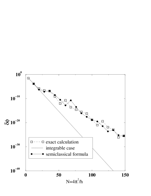
FIG. 1.: Eigenphase splitting for the kicked Harper system in the nearly integrable regime $(\tau=1)$. The splittings correspond to the Floquet mode whose WKB approximation quantizes on the classical torus with action $I_{\pi/4}=\pi/4$, for different values of $N=2\pi/\hbar$. Squares: exact numerical calculation. Filled circles: semiclassical approximation based on the resonance assisted tunneling mechanism. The doted line corresponds to the splitting for the integrable approximation. The solid and dashed lines are just guides to the eye.

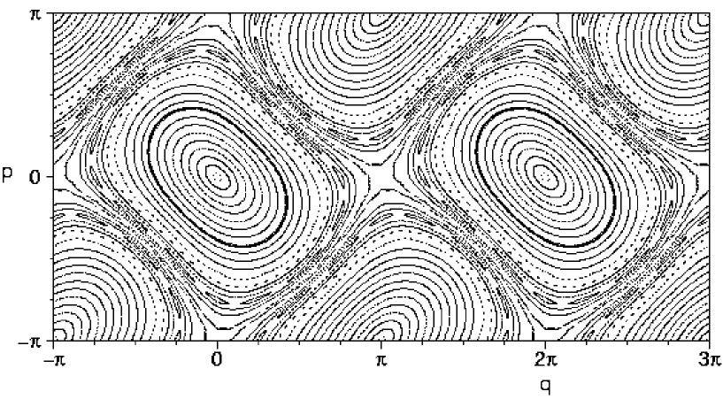
FIG. 2.: Poincaré section for the kicked Harper map Eq. (3) with $\tau=1$. The eigenphase splitting shown on Fig. 1 correspond to the tunneling processes between the quasimodes constructed on the tori with action I = pi/4 marked as thick lines in the left and right wells.

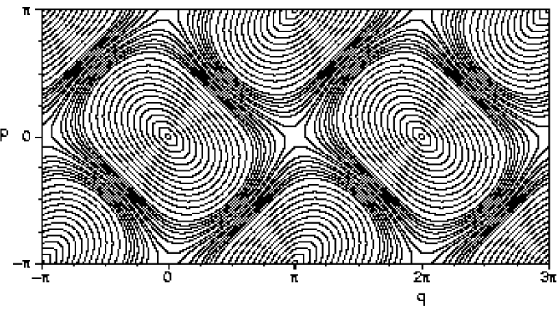
FIG. 3.: Poincaré section for the integrable approximation $\widetilde{H}^{(n)}$ with $n=6$ of the the kicked Harper map, see Eq. (15) at $\tau=1$. Note the good agreement between the invariant tori of this integrable system and the K.A.M. tori of the kicked Harper at $\tau=1$ (Fig. 2).

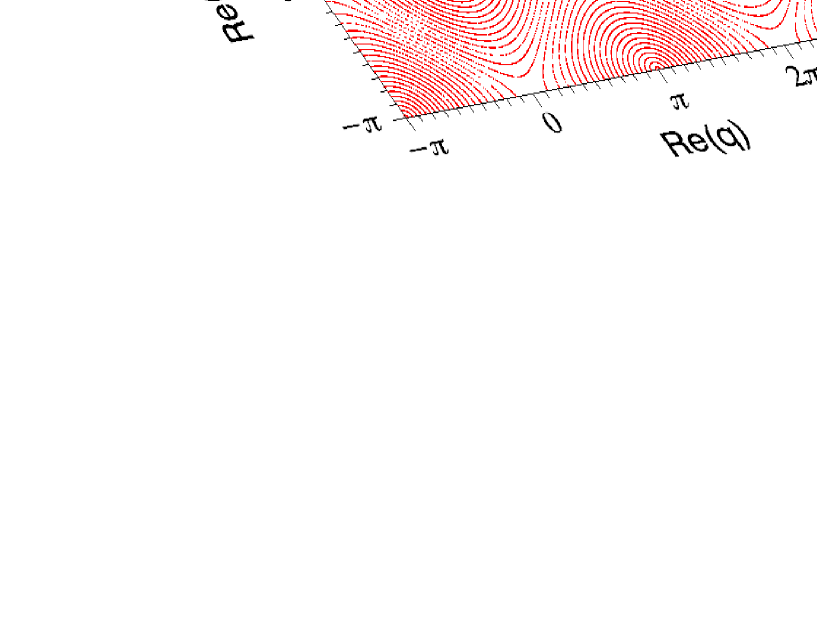
FIG. 4.: Part of the analytic continuation of an invariant torus and its symmetrically shifted counterpart for the integrable Harper hamiltonian. The imaginary part of momentum of the manifold is plotted versus the real parts of position and momentum, on top of the real phase space.

FIG. 5.: Part of the analytic continuation of a KAM torus and its symmetrically shifted counterpart in the near-integrable Kicked Harper at $\tau=1$. The imaginary part of momentum of the manifold is plotted versus the real parts of position and momentum, on top of the real phase space. In contrast to integrable dynamics, the two manifolds on each side of the separatrix do not join each other, but are interrupted far inside the regular phase space domain. Note the fluctuations that appear at the outermost end of the converged manifold (as shown in the inset for the manifold on the right hand side).

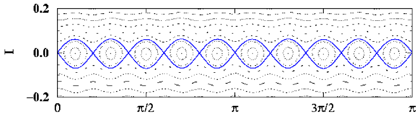
FIG. 6.: Poincaré section in the vicinity of the $10$:$1$ resonance of the kicked Harper, in the action angle variables of the integrable approximation $\widetilde{H}^{(n)}$ ($n=6$). Note the similarity of the phase space structure with the one of a generalized mathematical pendulum, with $10$ islands instead of one.

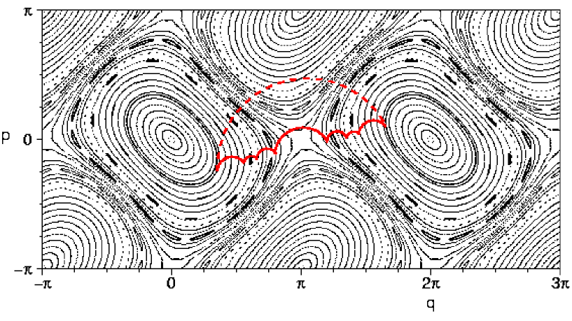
FIG. 7.: Visual representation of resonance-assisted tunneling: Plotted is, for the Kicked Harper system with $\tau=1$, the succession of complex paths that are used to accomplish the tunneling process for the 10th excited state at $2\pi/\hbar=126$. Instead of a direct transition (dashed curve) to the symmetry related torus, the quasi-mode is coupled via the $8$:$1$ (hardly visible) the $10$:$1$, and the $14$:$1$ resonance to the 50th excited state, which lies sufficiently close to the separatrix to tunnel with a large rate to its counterpart.

FIG. 8.: For the tenth iterate of a set of randomly distributed points in phase space, distance, as a function of the order of the approximation $n$, between the sets of resulting points depending on whether the kicked Harper or its integrable approximation $\widetilde{H}^{(n)}$ is used. The perturbation parameter is $\tau=1.0$.

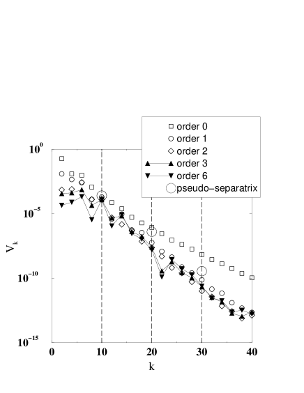
FIG. 9.: $k$-dependence of the resonance coefficients $V^{10:1}_{k}$ for the resonance $10$:$1$ of the kicked Harper with $\tau=1$. The various symbols correspond to different orders $n$ of the integrable approximation $\widetilde{H}^{(n)}$ used for the calculation, demonstrating the independence of the $V^{r:s}_{k}$ on $n$ for $n\simeq n_{0}=6$. The large circle symbols at $k=10,20,30$ show the result obtained for these Fourier coefficients with the pseudo-separatrix method used in [23].

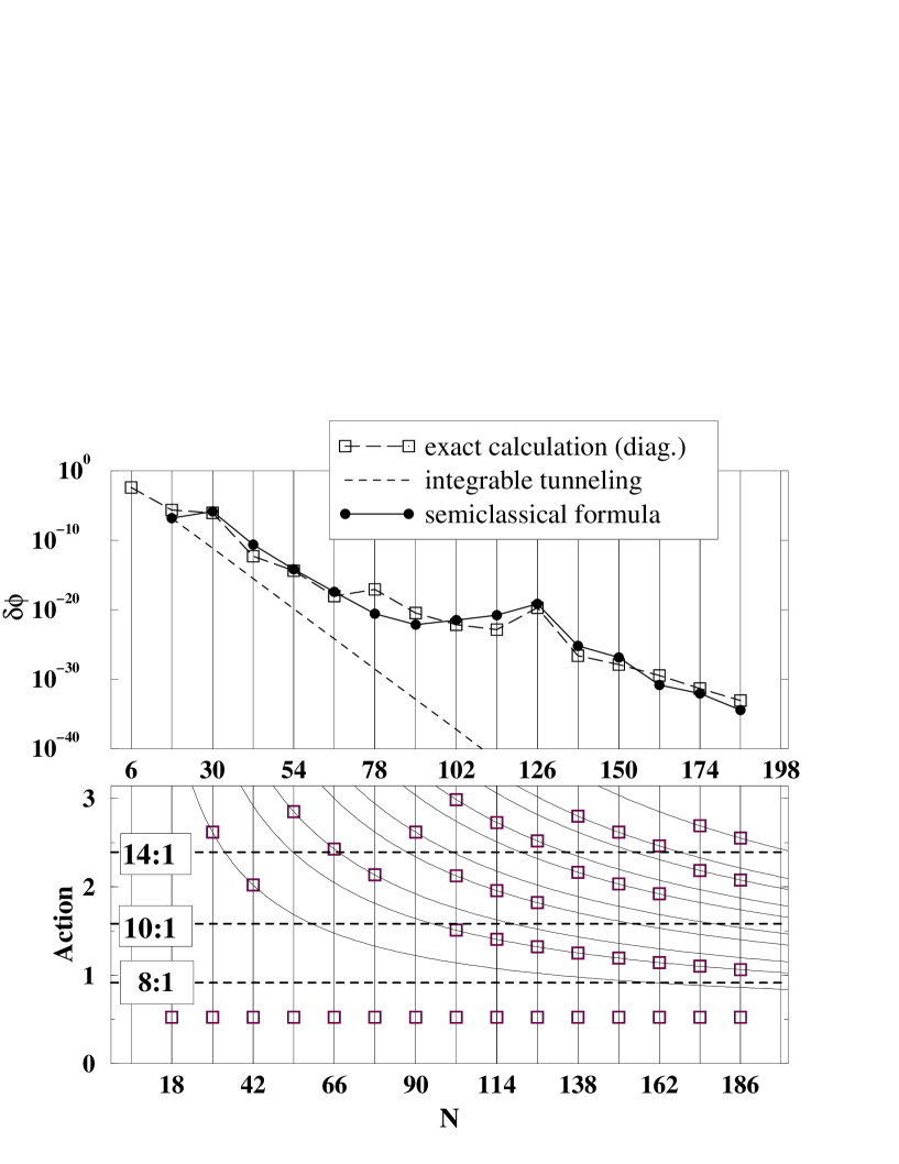
FIG. 10.: Top : same as Fig. 1, but for the Floquet mode whose WKB approximation quantizes on the classical torus with action $I_{\pi/6}=\pi/6$. Bottom : the classical action, for each value of $N$, of the modes involved in the dominant tunneling path. The horizontal doted line corresponds to the initial action $I_{\pi/6}$. The horizontal solid lines correspond to the actions of the resonances $8$:$1$, $10$:$1$ and $14$:$1$. The curved solid lines are such that $I-I_{\pi/6}={\rm const.}\times\hbar$ (that is, the distance from $I_{\pi/6}$ is constance in mode number unit). Notice that as $N=2\pi/\hbar$ increases, more resonances are involved.

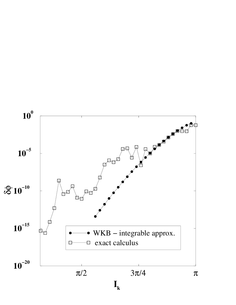
FIG. 11.: Eigenphase splitting for the kicked Harper system in the nearly integrable regime $(\tau=1)$, for a fixed value of $\hbar$ ($=2\pi/100$), and a variable initial torus. Squares: exact numerical calculations. Dots: integrable semiclassical approximation, without including the effect of the resonances. As the initial torus get close enough from the separatrix $I_{\rm max}=\pi$, the integrable approximation for the tunneling reproduces faithfully the exact quantum result, showing that the chaotic layer near the separatrix plays no role here.

FIG. 12.: For the order $n=2$ integrable approximation $\widetilde{H}^{(n)}$: comparison, as a function of the perturbation parameter $\tau$, of the fitted value $\vartheta_{\xi}$ of the slope of the log of the coefficient $V^{10:1}_{k}$ (squares) with the imaginary part of the angle coordinate of the visible singularities on the torus $I_{10:1}$ (circles) The lines are just guides to the eye.

FIG. 13.: Same as Fig. 12, but for the order $n=3$ integrable approximation $\widetilde{H}^{(n)}$.

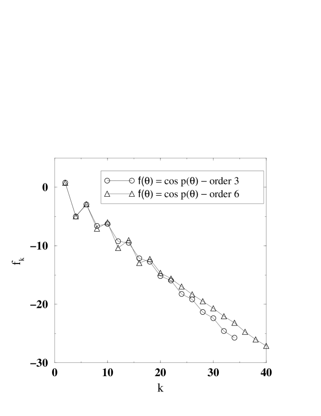
FIG. 14.: Fourier coefficients $f_{k}$ of the functions $f(\theta)=\cos\left[p(\theta,I_{10:1})\right]$. The different curves correspond to different orders $n$ of the integrable approximation used. We observe that although the $f_{k}$’s remain insensitive to the choice of the integrable approximation for not too large $k$, their asymptotic behavior differ depending on whether the integrable approximation with $n=3$ or $n=6$ is chosen.

FIG. 15.: Sorted complex orbit belonging to the outermost part of the continuation manifold shown in fig. 5. Plotted is the real part of momentum as a function of the pseudo angle $\theta$. One clearly recognizes significant periodic modulations of the orbit which appear on different scales, as can be seen from the magnifications shown in the insets.

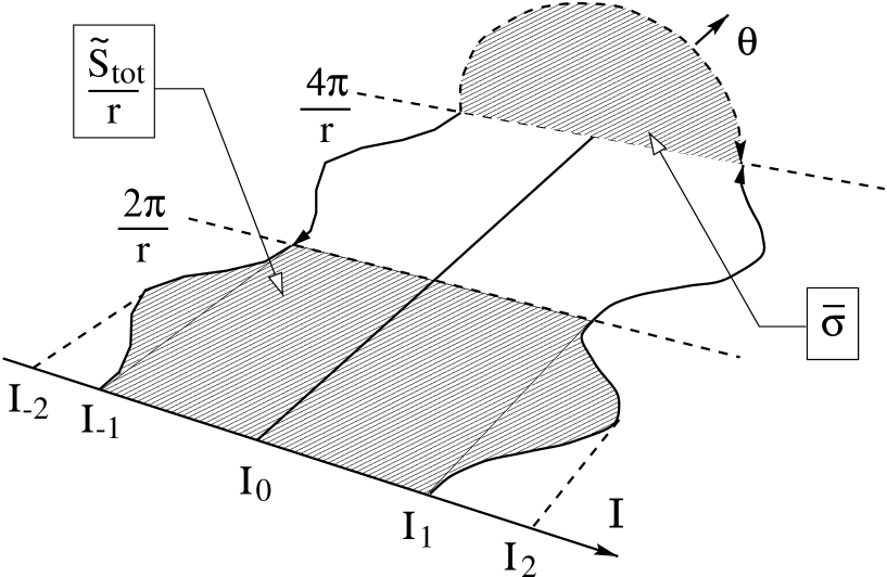
FIG. 16.: Sketch of the invariant manifold Eq. (C2) in complex phase space. The solid and interrupted lines belong respectively to the classically authorized and forbidden part of this manifold. The shaded area represent the action integral that parametrize the tunneling process.

REFERENCES

- [1] M. J. Davis and E. J. Heller, J. Chem. Phys. 75 (1981) 246.
- [2] J. Barnas and A. Fert Phys. Rev. Lett. 80, 1058-1061 (1998).
- [3] S. C. Creagh and N. D. Whelan, Phys. Rev. Lett. 77, 4975 (1996); and 82, 5237 (1999).
- [4] W. A. Lin and L.E. Ballentine, Phys. Rev. Lett. 65, 2927 (1990).
- [5] O. Bohigas, S. Tomsovic, D. Ullmo, Phys. Rep. 223, (1993) 43. O. Bohigas, D. Boosé, R. Egydio de Carvalho, and V. Marvulle, Nucl. Phys. A560 (1993) 197.
- [6] S. Tomsovic and D. Ullmo, Phys. Rev. E. 50 (1994) 145.
- [7] E. Doron and S.D. Frischat, Phys. Rev. Lett. 75, 3661 (1995). S.D. Frischat and E. Doron, Phys. Rev. E 57, 1421 (1998).
- [8] F. Leyvraz and D. Ullmo, J. Phys.A 29 (1996) 2529-2551.
- [9] J. Zakrzewski, D. Delande, A. Buchleitner Phys. Rev. E 57, 1458 (1998).
- [10] W. .K. Hensinger, et al., Nature 412, 52 (2001).
- [11] D. A. Steck, W. H. Oskay and M. G. Raizen, Science 293 274 (2001); Phys. Rev. Lett. 88, 120406 (2002).
- [12] A. Mouchet, C. Miniatura, R. Kaiser, B. Grémaud and D. Delande, Phys. Rev. E 64, 016221 (2001).
- [13] C. Dembowski et al., Phys. Rev. Lett. 84, 867 (2000).
- [14] J. U. Nöckel and A. D. Stone, Nature 385, 45 (1997).
- [15] J.M. Greene and I.C. Percival, Physica 3D, 530-548 (1981).
- [16] S. Creagh, in Tunneling in Complex Systems, edited by S. Tomsovic (World Scientific, Singapore, 1998), p. 35.
- [17] A. Shudo and K. S. Ikeda, Phys. Rev. Lett. 74, 682; Phys. Rev. Lett. 76, 4151. T. Onishi, A. Shudo, K. S. Ikeda, and K. Takahashi, Phys. Rev. E 64, 025201 (2001). A. Shudo, Y. Ishii and K. S. Ikeda, J. Phys. A:Math. Gen. 35 (2002) L1-L7.
- [18] L. Bonci, F. Farusi, P. Grigolini and R. Roncaglia, Phys. Rev. E 58 5689 (1998).
- [19] T. Uzer, D. W. Noid, and R. A. Marcus, J. Chem. Phys. 79, 4412 (1983).
- [20] A. M. Ozorio de Almeida, J. Phys. Chem. 88, 6139 (1984).
- [21] D. Farrely and T. Uzer, J. Chem. Phys. 85, 308 (1986).
- [22] H. P. Breuer and M. Holthaus, Ann. Phys. (N.J.) 211, 249 (1991).
- [23] O. Brodier, P. Schlagheck, and D. Ullmo, Phys. Rev. Lett. 87, 064101 (2001).
- [24] P. Leboeuf, J. Kurchan, M. Feingold, and D. P. Arovas, Phys. Rev. Lett. 65, 3076 (1990).
- [25] R. Lima and D. Shepelyansky, Phys. Rev. Lett. 67, 1377 (1991).
- [26] T. Geisel, R. Ketzmerick, and G. Petschel, Phys. Rev. Lett. 67, 3635 (1991).
- [27] R. Roncaglia, L. Bonci, F. Izrailev, B.J. West and P. Grigolini Phys. Rev. Lett. 73, 802 (1994).
- [28] V. V. Sokolov, Sov. J. Theor. Math. Phys. 67, 223 (1986). V. V. Sokolov, O. V. Zhirov, D. Alonso, and G. Casati, Phys. Rev. Lett. 84, 3566 (2000).
- [29] A. J. Lichtenberg and M. A. Lieberman, Regular and Stochastic Motion (Springer-Verlag, New York, 1983).
- [30] F. Grossmann, T. Dittrich, P. Jung, and P. Hänggi, Phys. Rev. Lett. 67 (1991) 516.
- [31] Memoirs of the American Mathematical Society 81: Lectures on Hamiltonian systems by Jürgen Moser.
- [32] V.P. Maslov and M.V. Fedoriuk, Semiclassical approximation in quantum mechanics, (Reidel, Dordrecht,1981) [original Russian edition 1965].
- [33] See e.g. appendices 10 and 11 of : V.I. Arnold, Mathematical methods of classical mechanics, Springer Verlag, 1978.
- [34] L. Landau et E. Lifchitz, Mécanique Quantique, Éditions Mir 1966.
- [35] S. C. Creagh, J. Phys. A 27, 4969 (1994).
- [36] B. V. Chirikov, Phys. Rep. 52, 265 (1979).
- [37] M. Wilkinson, Physica 21D, 341 (1986); J. Phys. A 20, 635 (1987).
- [38] R. E. Langer, Phys. Rev. 51, 669 (1937).
- [39] We should note that that we cannot rigourously show Eq. (47) to hold in the extreme perturbative regime. The matching between the semiclassical and the quantum transition amplitudes is therefore not necessarily expected.
- [40] E. B. Bogomolny, Physica 13D, 281-301 (1984).