Solitons in Triangular and Honeycomb Dynamical Lattices with the Cubic Nonlinearity

Abstract

We study the existence and stability of localized states in the discrete nonlinear Schrödinger equation (DNLS) on two-dimensional non-square lattices. The model includes both the nearest-neighbor and long-range interactions. For the fundamental strongly localized soliton, the results depend on the coordination number, i.e., on the particular type of the lattice. The long-range interactions additionally destabilize the discrete soliton, or make it more stable, if the sign of the interaction is, respectively, the same as or opposite to the sign of the short-range interaction. We also explore more complicated solutions, such as twisted localized modes (TLM’s) and solutions carrying multiple topological charge (vortices) that are specific to the triangular and honeycomb lattices. In the cases when such vortices are unstable, direct simulations demonstrate that they turn into zero-vorticity fundamental solitons.

today

I Introduction

In the past decade, energy self-localization in nonlinear dynamical lattices, leading to the formation of soliton-like intrinsic localized modes (ILMs), has become a topic of intense theoretical and experimental research. Much of this work has already been summarized in several reviews [1, 2, 3, 4, 5, 6]. It was proposed that this mechanism would be relevant to a number of effects such as nonexponential energy relaxation in solids [7], local denaturation of the DNA double strand [8, 9, 10, 11], behavior of amorphous materials [12, 13, 14], propagation of light beams in coupled optical waveguides [15, 16, 17] or the self-trapping of vibrational energy in proteins [18], among others. ILMs also have potential significance in some crystals, like acetanilide and related organics [19, 20]. The theoretical efforts were complemented by a number of important experimental works suggesting the presence and importance of the ILMs in magnetic [21] and complex electronic materials [22], DNA denaturation [23], as well as in coupled optical waveguide arrays [24, 25] and Josephson ladders [26, 27].

A ubiquitous model system for the study of ILMs is the discrete nonlinear Schrödinger (DNLS) equation (see e.g., the review [6] and references therein). Within the framework of this model and, more generally, for Klein-Gordon lattices, it has recently been recognized that physically realistic setups require consideration of the ILM dynamics in higher spatial dimensions [28, 29, 30, 32, 33, 34, 35, 36, 37]. In the most straightforward two-dimensional (2D) case, almost all of these studies, with the exception of Refs. [38, 39] were performed for square lattices. However, it was stressed in Ref. [38, 39] that non-square geometries may be relevant to a variety of applications, ranging from the explanation of dark lines in natural crystals of muscovite mica, to sputtering (ejection of atoms from a crystal surface bombarded by high-energy particles), and, potentially, even to high-temperature superconductivity in layered cuprates. Besides that, it has been well recognized that triangular (TA) and hexagonal (or honeycomb, HC) lattices are relevant substrate structures in a number of chemical systems [40] and, especially, in photonic band-gap (PBG) crystals [41, 42]. Notice that, in the context of the PBG crystals, the relevance of nonlinear effects has been recently highlighted for a square diatomic lattice [43].

The above discussion suggests the relevance of a systematic study of ILMs in the paradigm DNLS model for TA and HC lattices. The aim of the present work is to address this issue (including the stability of the ILM solutions), for the 2D lattices with both short-range and long-range interactions. In section II we discuss the effects of the non-square lattice geometry on the fundamental ILM state (the one centered on a lattice site), and then explore effects of long-range interactions on this state. In section III, we expand our considerations to other classes of solutions, which are either more general ones, such as twisted modes, which are also known in square lattices, or represent states that are specific to the TA and HC structures, viz., discrete vortices. We identify stable fundamental vortices in the TA and HC lattices with vorticity (spin) $S=3$ and $S=5$, and with the hexagonal and honeycomb shape, respectively. Additionally, a triangular vortex is found in the HC lattice, but it is always unstable.

II Fundamental intrinsic localized modes

A The model

In this work we consider the two-dimensional DNLS equation with the on-site cubic nonlinearity,

$$i\dot{\psi}_{nm}=-C\sum_{\left\langle n^{\prime},m^{\prime}\right\rangle}\psi_{n^{\prime}m^{\prime}}+kC\psi_{nm}-|\psi_{nm}|^{2}\psi_{nm}-\sum_{n^{\prime},m^{\prime}}{\bf K}\left(h\sqrt{(n-n^{\prime})^{2}+(m-m^{\prime})^{2}}\right)\psi_{n^{\prime}m^{\prime}}\,,$$ (1)

The subscripts ($n,m$) attached to the complex (envelope) field $\psi$ are two discrete spatial coordinates, $C$ is the constant of the linear coupling between nearest-neighbor sites, the summation over which is denoted by $\left\langle...\right\rangle$, and $k$ is the coordination number (i.e., the number of the nearest neighbors), which takes the values $k=6$ for the TA lattice (see the left panel of Fig. 1), $k=4$ for the square lattice, and $k=3$ for the HC one (see the right panel of Fig. 1). The function ${\bf K}$ represents a kernel of the long-range linear coupling, and $h\equiv 1/\sqrt{C}$ is the lattice spacing.

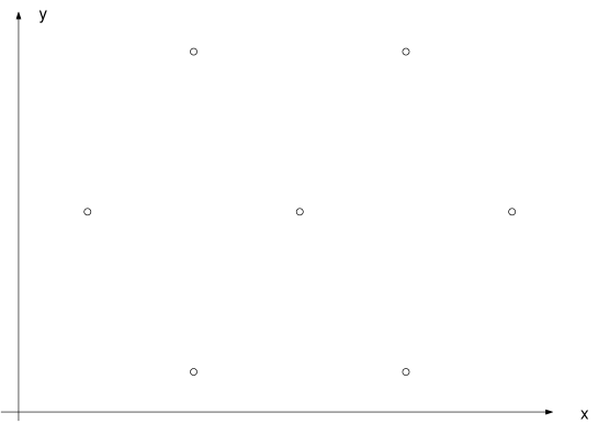
FIG. 1.: The top panel shows a cell of the triangular configuration incorporating six nearest neighbors of a given site. Similarly, one of the two possible configurations of neighbors in the honeycomb lattice is shown in the bottom panel. An alternative possibility in the latter case involves one neighbor along the negative y-axis and two neighbors along directions at $\pm\pi/3$ angles with the positive y-axis (if we place the central site at the origin of the coordinate system).

It is worth noting here that the TA network is a simple Bravais lattice with the coordinates of the grid nodes $x_{nm}=h(n+m/2)$ and $y_{nm}=\sqrt{3}hm/2$ (see also Ref. [41]). The same is true for the most commonly used square lattice, which has $x_{nm}=nh$, $y_{nm}=mh$, but not for the HC structure, a simple representation of which (for $h=1$) is $x_{nm}=\sqrt{3}m$ , $y_{nm}=(1/4)\left[6n-5+(-1)^{n+m}\right]$. More information on the latter structure (which also represents, for instance, the arrangement of carbon atoms in a layer of graphite) and its symmetries can be found in Ref. [44].

First, we will look for ILM solutions of the nearest-neighbor version of the model, setting ${\bf K}\equiv 0$. Stationary solutions with a frequency $\Lambda$ are sought for in the ordinary form (see e.g., Ref. [6]),

$$\psi_{nm}=\exp(i\Lambda t)\,u_{nm}\,.$$ (2)

The substitution of Eq. (2) into Eq. (1) leads to a time-independent equation for the amplitudes $u_{mn}$. The stationary solution being known, one can perform the linear-stability analysis around it in the same way as it has been done for the square lattice [45, 46, 47], assuming a perturbed solution in the form

$$\psi_{nm}=\exp(i\Lambda t)(u_{nm}+\epsilon w_{nm}),$$ (3)

where $w_{nm}$ is a perturbation with an infinitesimal amplitude $\epsilon$. Deriving the leading-order equation for $w_{nm}$, and looking for a relevant solution to it in the form $w_{nm}=a_{nm}\exp(-i\omega t)+b_{nm}\exp(i\omega_{nm}^{\star}t)$ (where the eigenfrequency $\omega$ is, generally speaking, complex), one arrives at an eigenvalue problem for $\{\omega,\left(a_{nm},b_{nm}^{\star}\right)\}$:

$$\omega a_{nm} = -C\sum_{<n^{\prime},m^{\prime}>}a_{n^{\prime},m^{\prime}}+kCa_{nm}-2|u_{nm}|^{2}a_{nm}+\Lambda a_{nm}-u_{nm}^{2}b_{nm}^{\star},$$ (4)

$$-\omega^{\star}b_{nm} = -C\sum_{<n^{\prime},m^{\prime}>}b_{n^{\prime},m^{\prime}}+kCb_{nm}-2|u_{nm}|^{2}b_{nm}+\Lambda b_{nm}-u_{n,m}^{2}a_{nm}^{\star}.$$ (5)

The inclusion of long-range effects into the linear-stability equations is straightforward. As the long-range coupling is accounted for by a linear operator acting on the complex field, terms $-{\bf K}\left(h\sqrt{(n-n^{\prime})^{2}+(m-m^{\prime})^{2}}\right)a_{n^{\prime}m^{\prime}}$ and $-{\bf K}\left(h\sqrt{(n-n^{\prime})^{2}+(m-m^{\prime})^{2}}\right)b_{n^{\prime}m^{\prime}}$ are to be added to Eqs. (4) and (5), respectively.

B ILMs in the models with the nearest-neighbor interactions

Fundamental (single-site-centered) ILM solutions to the stationary equations were constructed by means of a Newton-type method, adjusted to the non-square geometry of the TA and HC lattice. For the results presented herein, we fix the frequency to be $\Lambda=1$ and vary the coupling constant $C$, as one of the two parameters ($\Lambda$ and $C$) can always be scaled out from the stationary equations. We started from obvious single-site solutions (with $|u|=\sqrt{\Lambda}\equiv 1$) at the anti-continuum limit corresponding to $C=0$ [48], and then continued the solution to finite $C$. Subsequently, the stability analysis was performed using Eqs. (4)-(5) for the corresponding lattice.

Typical examples of stable and unstable fundamental ILMs found in both the TA and HC lattices are displayed, by means of contour plots, in Fig. 2. The top panel of the figure shows, respectively, stable and unstable solutions, together with the associated spectral-plane diagrams (showing the imaginary vs. real parts of the eigenfrequencies), for the TA lattice with $C=0.1$ (top subplots) and $C=0.7$ (bottom subplots). Stable and unstable solutions in the HC lattice are shown in the bottom panel of Fig. 2 for $C=0.1$ (top subplots) and at $C=1.6$ (bottom subplots).

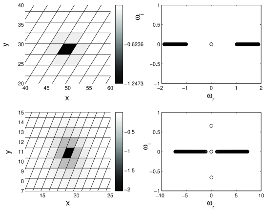
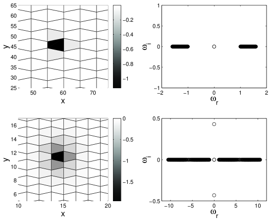
FIG. 2.: Single-site-centered fundamental ILMs in the triangular and honeycomb lattices. In the top panel of the figure, the solutions in the triangular lattice are displayed for two cases: $C=0.1$ in the top row, and $C=0.7$ in the bottom row. The left subplot in each case shows a checkerboard contour plot of the solution proper, and the right subplot shows the spectral plane ($\omega_{r},\omega_{i}$) of the corresponding eigenfrequencies $\omega$ (the subscripts ${\rm r}$ and ${\rm i}$ stand for the real and imaginary part of the eigenfrequency). It is seen that the solution is stable for $C=0.1$, and unstable for $C=0.7$. Similar results are displayed in the bottom panel of the figure for the honeycomb lattice. A stable solution is shown for $C=0.1$ in the top row, and an unstable one for $C=1.6$ in the bottom row. Notice that the contour plots show a “negative image” of the solution. The grayscale in all the contour plots presented in this work is used to denote amplitude.

A natural way to understand the stability of the ILMs is to trace the evolution and bifurcations of the eigenfrequencies and associated eigenmodes with the increase of the nearest-neighbor coupling $C$. For the square lattice, we find, in line with results of Refs. [28, 36], that a bifurcation generating an internal mode from the edge of the continuous spectrum (the edge is at $\omega=\Lambda\equiv 1$) in the corresponding ILM occurs at a critical value $C=0.4486$. As the coupling is further increased, the pair of the corresponding eigenfrequencies moves towards the origin of the spectral plane, where they collide and bifurcate into an unstable pair of imaginary eigenfrequencies at $C=\Lambda$ (i.e., at $C\equiv 1$ in the present notation), so that the ILM in the square lattice is unstable for $C>1$.

In the TA and HC lattices, the scenario is found to be quite similar. For the former lattice, the bifurcation of the two eigenfrequencies from the continuous band edge (which is depicted by the dash-dotted line) and their trajectory, as they change from real, i.e., stable (the solid line) into imaginary, i.e., unstable (the dashed line), are shown in the top panel of Fig. 3. The bottom panel shows the same trajectory for the HC lattice. The pair of eigenvalues bifurcates at $C=0.2974$ in the TA lattice, and they reach the origin, giving rise to the instability, at a point close to $C=0.63$. In the HC lattice, the bifurcation giving rise to the originally stable eigenvalues occurs at $C=0.6247$; they collide at the origin and become unstable at $C=1.505$.

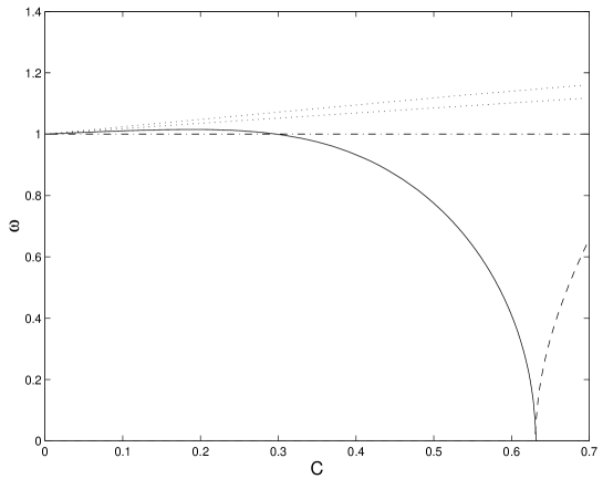
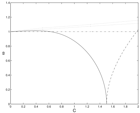
FIG. 3.: The top panel shows the evolution of the two eigenfrequencies of the fundamental ILM in the triangular lattice. The eigenvalues bifurcate from the edge of the continuous spectrum (at $C=0.2974$) and move towards the origin, which they hit at $C\approx 0.63$, giving rise to an unstable pair of imaginary eigenfrequencies. The absolute value of the eigenfrequencies is shown by the solid line when they are real (stable), and by the dashed line when they are imaginary (unstable). The dash-dotted line indicates the edge of the continuous-spectrum band. The bottom panel shows the same for the ILM in the honeycomb lattice. In this case, the stable eigenvalues appear at $C\approx 0.6247$, and they become unstable imaginary ones, hitting the origin at $C=1.505$. In both panels, the two next pairs of eigenvalues (which are always found inside the phonon band) are also shown for comparison by the dotted lines.

One can clearly identify the effect of geometry in these results. In particular, since the instability occurs beyond the critical values of the coupling, it is the linear interaction between the neighbors that drives it. Consequently, since the coordination numbers for the different lattices are ordered as $k_{{\rm triang}}>k_{{\rm square}}>k_{{\rm honey}}$, the instability thresholds (critical values of the coupling constant) for these lattices should be ordered conversely, $C_{{\rm triang}}^{{\rm(cr)}}<C_{{\rm square}}^{{\rm(cr)}}<C_{{\rm honey}}^{{\rm(cr)}}$. A similar understanding of the effect of the coordination number on the norm of the solution, $N\equiv\sum_{m,n}\left|u_{mn}\right|^{2}$, justifies the results displayed in Fig. 4: the larger number of neighbors endows the TA branch (solid line) with a larger norm than the square one (dash-dotted), which, in turn, has a larger norm than the HC lattice (dashed).

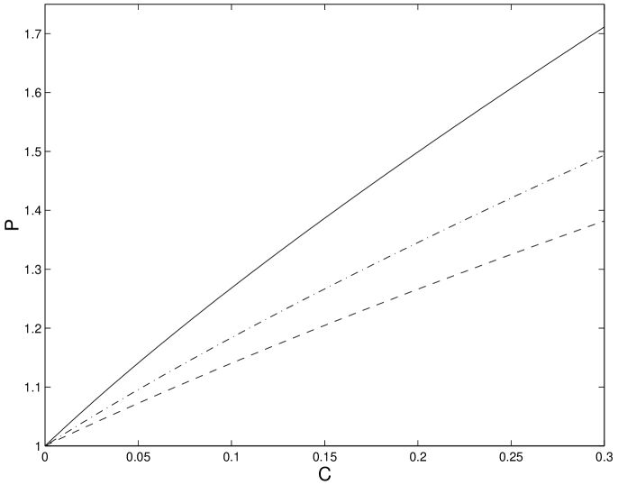
FIG. 4.: The norm of the fundamental ILM solutions in the TA, square and HC lattices vs. the coupling constant. The triangular-, square-, and honeycomb-lattice branches are shown, respectively, by the solid, dash-dotted, and dashed lines.

C ILMs in the lattices with the long-range interaction

Recently, a lattice model with a long-range coupling, which is relevant to magnon-phonon, magnon-libron and exciton-photon interactions, was introduced in Ref. [49]. In the framework of this model, it has been concluded that the relevant coupling kernel [see Eq.(1)] is

$${\bf K}\left(h\sqrt{(n-n^{\prime})^{2}+(m-m^{\prime})^{2}}\right)=F_{0}K_{0}\left(\alpha h\sqrt{(n-n^{\prime})^{2}+(m-m^{\prime})^{2}}\right),$$ (6)

where $F_{0}$ is an amplitude of the kernel, $\alpha^{-1}$ measures the range of the interaction, and $K_{0}$ is the modified Bessel function. We will use this kernel below.

Inserting the kernel (6) into Eq. (1), one can see how the behavior of the branch is modified as a function of $F_{0}$ for a given fixed value of the nearest-neighbor coupling $C$. Notice that similar results (but on a logarithmic scale) will be obtained if $\alpha$ is varied, while $F_{0}$ is kept fixed, as it was detailed in Ref. [49]. Thus, we fix $\alpha=0.1$ hereafter.

In Fig. 5, we show the evolution of the numerically found internal-mode eigenvalues of ILM as a function of $F_{0}$, for fixed $C=0.1$ . It can be observed that the increase of $F_{0}$ leads to an instability for $F_{0}>0.01425$. The bottom panel shows the configuration and its internal-eigenmode frequency for $F_{0}=0.015$, when the configuration is already unstable. Carefully zooming into the ILM’s in the case of long-range interactions (data not shown here), one can notice a “tail” of the ILM, much longer than the size of the ILM in the case of the nearest-neighbor interaction, which is a natural consequence of the nonlocal character of the interaction in the present case. For $F_{0}>0$, we thus conclude that the long-range interaction “cooperates” with the short-range one, lowering the instability threshold. On the contrary, numerical results for $F_{0}<0$ show that the onset of the instability is delayed when the long- and short-range interactions compete with each other (see also Ref. [49]).

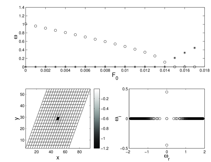
FIG. 5.: Top panel: the variation of the internal-mode eigenfrequency $\omega$ for the fundamental ILM vs. the amplitude of the long-range interaction $F_{0}$ for $C=0.1$. The stars and circles denote the real and imaginary parts of the eigenvalue. It can be seen that, while the ILM is stable at $F_{0}=0$, an instability sets in at $F_{0}=0.01425$. The left part of the bottom panel shows the (unstable) ILM configuration, in a pseudocolor contour plot (of the amplitude), and the corresponding spectral plane ($\omega_{r},\omega_{i}$)) of the eigenmodes is shown in the right part. These results pertain to the triangular lattice. Once again, the contour plot shows the “negative image” of the solution, for clarity.

One can extend the above considerations to the case where both $F_{0}$ and $C$ are varied and construct two-parameter diagrams, separating stability and instability regions. An example is shown for the TA lattice in Fig. 6. For a fixed $C$, the critical value $\left(F_{0}\right)_{{\rm cr}}$ was identified, beyond which the ILM is unstable. Thus, in Fig. 6 ILM’s are stable below the curve and unstable above it.

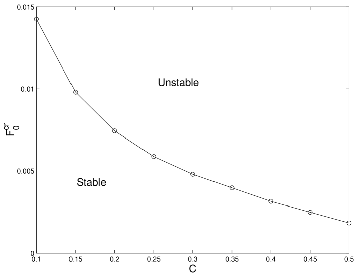
FIG. 6.: A two-parameter stability diagram for the ILM in the model combining the long- and short-range interactions. The stability region is located beneath the curve. The results pertain to the triangular lattice. For the honeycomb lattice, the stability region is quite similar.

III Multiple-Site ILM’s

We now turn our attention to solutions comprising many sites of the lattice. In this case too, the solutions are initially constructed in the anti-continuum limit $C=0$, and then extended through continuation to finite values of $C$.

A Twisted localized modes

Firstly, we examine the so-called twisted localized modes (TLMs), which were originally introduced, in the context of 1D lattices, in Refs. [50, 51]. Later, they were studied in more detail in Ref. [52], and their stability was analyzed in Ref. [53]. They were subsequently used to construct topologically charged 2D solitons (vortices) in the square-lattice DNLS equation in [54].

In the case of the square lattice, and subject to the same normalization as adopted above, i.e., with $\Lambda=1$, TLMs are found to be stable for $C<0.125$. If the coupling exceeds this critical value, an oscillatory instability, which is manifested through a quartet of complex eigenvalues [55], arises due to the collision of the TLM’s internal mode with the continuous spectrum (the two have opposite Krein signatures [2, 47]), as it has been detailed in Ref. [53]. The same scenario is found to occur in the TA lattice. However, in the latter case the oscillatory instability sets in at $C\approx 0.1$, and the destabilization is a result of the collision of the eigenvalues with those that have (slightly) bifurcated from the continuous spectrum (rather than with the edge of the continuous spectrum at $\omega=1$, as in the square lattice).

Similarly, in the HC lattice, the instability of TLMs sets in at $C=0.1375$. Notice that the instability thresholds follow the same ordering as the ones discussed in the previous section. This can be justified by a similar line of arguments as given before. The TLM in the TA lattice (and its stability) is displayed in the top panel of Fig. 7 for $C=0.2$, which exceeds the instability threshold. The bottom panel of the figure shows the variation (as a function of the coupling $C$) of the critical eigenfrequency. The real stable eigenfrequency, and the imaginary part of the unstable ones, after the threshold has been crossed, are shown, respectively, by solid and dashed lines. Figure 8 displays analogous results for the HC lattice. The solution is shown at $C=0.2$ in the top panel.

It should be remarked that, in the 2D lattice, the TLMs are solutions carrying vorticity (topological charge) $S=1$ [54] (although they are different from vortices proper, see below). The simplest way to see this is by recognizing that TLM configurations emulate the continuum-limit expression $\cos\theta$, where $\theta$ is the angular coordinate in the 2D plane, i.e., the real part of $\exp(i\theta)$, the latter expression carrying vorticity $1$. It should also be added that, after the onset of the oscillatory instability, TLM solutions have been found to transform themselves into the fundamental (single-site-centered) ILM configurations, which is possible as the topological charge is not a dynamical invariant in lattices [54, 56].

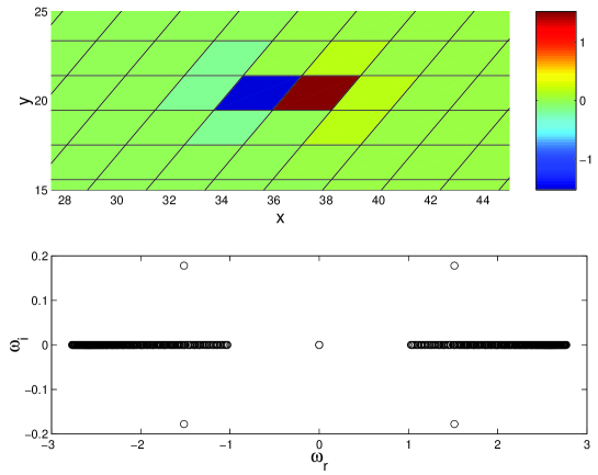
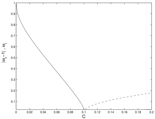
FIG. 7.: The top panel shows the solution (top subplot) and its stability (bottom subplot) for a TLM in the triangular lattice at $C=0.2$. One can readily observe the presence of the oscillatory instability in the eigenfrequency spectrum. The bottom panel shows the critical eigenfrequency vs. the coupling constant $C$. The solid line shows the distance of the eigenfrequency from the band edge of the continuous spectrum. After the collision, which takes place at $C=0.1$, a quartet of complex eigenvalues emerges; the absolute value of their imaginary part is shown by the dashed line.

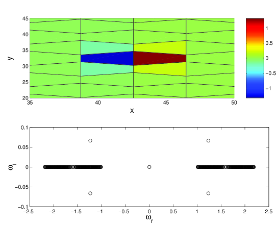
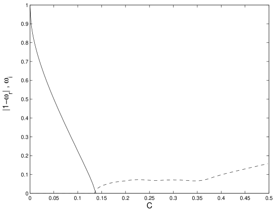
FIG. 8.: The same as Fig. 7, but for the honeycomb  lattice. The top panel shows the solution at $C=0.2$; the bottom panel shows the distance of the internal mode eigenfrequency from the band edge (solid line), and the absolute value of the imaginary part of the eigenvalue quartet for $C>0.1375$ (dashed line).

B Hexagonal and triangular vortex solitons

Going beyond TLMs, it is appropriate to consider possible lattice solitons which conform to the symmetry of the TA or HC lattice. In fact, these are the most specific dynamical modes supported by the lattices. An example of this sort in the TA lattice are “hexagonal” ILMs shown in Fig. 10 . The top panel of the figure shows the profile of these modes in the anti-continuum limit, and the bottom panel displays two actual examples of these modes. The top subplot shows the hexagonal ILM for $C=0.038$, when it is stable, while the bottom subplot shows the mode at $C=0.218$, after the onset of three distinct oscillatory instabilities. The first and second instabilities set in at $C\approx 0.064$ and $C\approx 0.084$ respectively, while the final eigenvalue quartet appears at $C\approx 0.184$.

Measuring the topological charge of this solution around the contour in the top panel of Fig. 9, we find (since each jump from $+1$ to $-1$ can be identified as a $\pi$ phase change) that the whole solution has a total phase change of $6\pi$, hence its topological charge (vorticity, or “spin”) is $S=3$. Then, the presence of three oscillatory instabilities agrees with a recent conjecture [56], which states that the number of negative-Krein-sign eigenvalues (and hence the number of potential oscillatory instabilities) coincides with the topological charge of the 2D lattice soliton. However, if one examines more carefully the stability picture, one finds that, due to the symmetry of the solution, two of these eigenvalues have multiplicity $2$. Hence, the conjecture needs to be refined, to take into regard the potential presence of symmetries. The thus revised conjecture states that the topological charge of the solution should be equal to the geometric (but not necessarily algebraic) multiplicity of the eigenvalues with negative Krein signature.

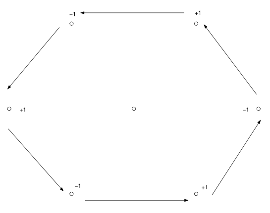
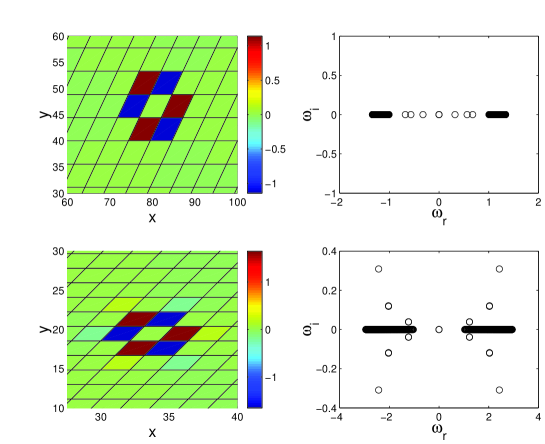
FIG. 9.: The top panel shows the anti-continuum-limit profile of the topologically charged hexagonal ILM in the triangular lattice (and a contour around the solution; each line in the contour represents a phase change by $\pi$). The bottom panel shows two examples of such a soliton. The solution is in each case shown in a pseudocolor contour plot on the left, while its eigenfrequency spectrum is shown on the right. The top subplot of the bottom panel corresponds to the stable soliton at $C=0.038$, while the bottom subplot represents an unstable one at $C=0.218$. In the latter case, three (in terms of the geometric multiplicity; the algebraic multiplicity is five) quartets of eigenvalues have become unstable.

It is natural to ask then to what configuration this hexagonal ILM will relax once it becomes unstable. To address the issue, we performed direct numerical simulations for $C=0.218$. Results are shown in our subplots of Fig. 10. In particular, the top left panel shows the solution at $t=200$ (the configuration at $t=0$ was the unstable hexagonal ILM). It can clearly be observed that the instability that sets in around $t\approx 50$ (according to the other three subplots) transforms the hexagonal vortex into a fundamental (zero-vorticity) ILM; recall that such an outcome of the instability development is possible because the vorticity is not conserved in lattice systems [54].

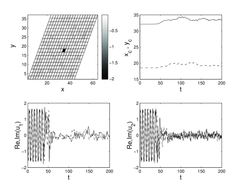
FIG. 10.: The time evolution of the unstable solution from the previous figure (for $C=0.218$) is shown here for the triangular lattice. The top left panel shows the solution at $t=200$. The “negative image” of the solution is shown once again for clarity. The top right panel shows the time evolution of the center-of-mass coordinates of the soliton, defined as $x_{c}\equiv\sum_{n,m}n|u_{n,m}|^{2}/\sum_{n,m}|u_{n,m}|^{2}$, $y_{c}\equiv\sum_{n,m}m|u_{n,m}|^{2}/\sum_{n,m}|u_{n,m}|^{2}$. The two bottom panels show the evolution of the real (solid line) and imaginary (dashed line) parts of the lattice field at two sites closest to the soliton’s center (subscripts $1$ and $2$ pertain, respectively, to the sites $n=10,m=11$ and $n=10,m=9$). A clear conclusion is that the instability sets in at $t\approx 50$, and it eventually results in the transformation of the hexagonal ILM into a stable fundamental ILM localized around a single lattice site.

For the HC lattice, a vortex soliton of a triangular form was found, see an example in Fig. 11 for $C=0.09$. We have found that this solution is unstable for all values of $C$.

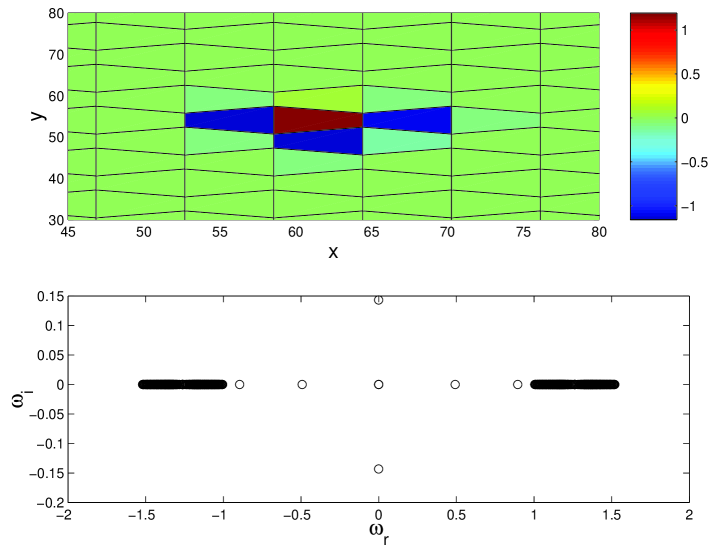
FIG. 11.: A triangular ILM solution in the honeycomb lattice, and the corresponding spectral plane, are shown for $C=0.09$. Solutions of this type were found to be unstable for all values of $C$.

Another vortex soliton, with a honeycomb shape, was also found in the HC lattice, see Fig. 12. This one is stable at a sufficiently weak coupling. If a contour is drawn around this solution (shown in the top panel of the figure for the anti-continuum limit), the net phase change is found to be $10\pi$, hence the corresponding topological charge is $S=5$. In accordance with the conjecture mentioned above, when the solution is stable, we find five internal modes with negative Krein signature. These modes eventually lead, as the coupling is increased, to five oscillatory instabilities. In the bottom panel of Fig. 12, the top subplot shows the case with $C=0.0475$, when the honeycomb-shaped vortex soliton in the HC lattice is linearly stable. The bottom subplot features the presence of five eigenvalue quartets in the case $C=0.43$, when all five oscillatory instabilities have been activated. The first instability occurs at $C=0.085$, the second at $0.1$, the third at $0.1375$, the fourth at $0.2025$, and the fifth sets in at $C=0.4025$.

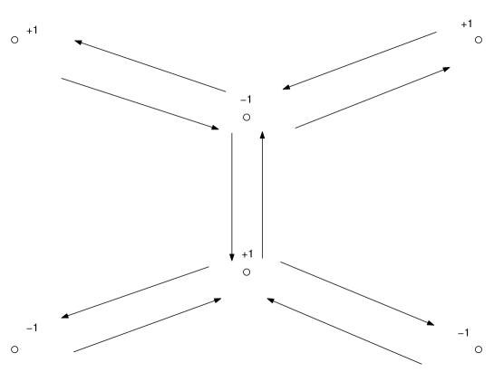
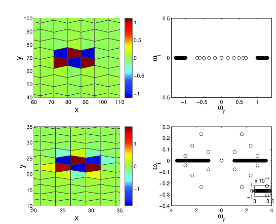
FIG. 12.: The top panel shows the profile of the honeycomb-shaped ILM in the anti-continuum limit in the honeycomb lattice, together with a contour around the solution. Each line in the contour represents a phase change by $\pi$, adding up to $10\pi$, hence the solution has vorticity $S=5$. An actual solution is shown in the bottom panel for $C=0.0475$, when it is linearly stable, having five negative-Krein-signature internal modes (top subplot). The bottom subplot of the bottom panel pertains to the case $C=0.43$, where all five oscillatory instabilities have developed. Four quartets of eigenfrequencies are clearly discernible. The fifth quartet is shown in the inset of the corresponding spectral-plane plot.

To illustrate the result of the development of the instability of the latter vortex in the case in which it is unstable, we have again resorted to direct numerical integration of Eq. (1). An example is shown in Fig. 13 for $C=0.43$. At $t\approx 500$, only one main pulse is sustained. Hence, in this case too, the multiply charged topological soliton is transformed, through the instability, into the stable (for this value of $C$) fundamental zero-vorticity ILM.

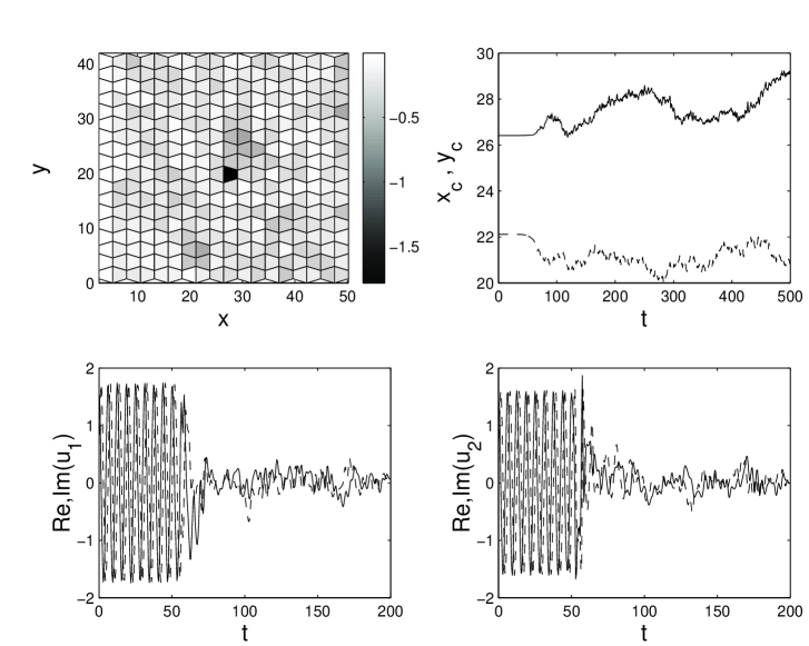
FIG. 13.: The evolution of the unstable honeycomb-shaped ILM configuration for $C=0.43$. The panels have the same meaning as in Fig. 10. The lattice-field configuration is shown in the top left panel for $t=500$. One predominant single-site pulse is present in the configuration. The other three panels show the time evolution of the center-of-mass coordinates and of the real and imaginary parts of the field at specific lattice sites (as in Fig. 10), clearly indicating that the instability sets in at $t\approx 60$.

IV Conclusion

In this work, we have studied a paradigm nonlinear lattice dynamical model, namely the DNLS equation, in two spatial dimensions for non-square lattices. The triangular and honeycomb networks were considered, as the most important examples of Bravais and non-Bravais 2D lattices, which are relevant to chemical and optical applications.

In the case of nearest-neighbor interactions, it was found that the instability thresholds for the fundamental solution centered at a single lattice site depend on the coordination number. The instability appears in the triangle lattice at a smaller value of the coupling constant than in the square lattice, while the opposite is true for the honeycomb lattice. The effect of the long-range interactions was also examined in this context. It was found that these interactions accelerate or delay the onset of the instability if they have the same sign as the nearest-neighbor coupling, or the opposite sign. Diagrams in the two-parameter plane were constructed, identifying regions of stability and instability in the presence of both the short- and long-range coupling.

More complicated lattice solitons, which essentially extend to several lattice sites, were also examined. A prototypical example of the extended solitons are twisted modes, for which the phenomenology was found to be similar to that in the square lattice, but with, once again, appropriately shifted thresholds. We have also examined solutions with a higher topological charge, which play the role of fundamental vortices in the triangular and honeycomb lattices, their vorticity being, respectively, $S=3$ and $S=5$. Stability of these vortices was studied in detail. When instabilities occurred, their outcome was examined by means of direct time integration, showing the transformation into a simple fundamental soliton with zero vorticity.

Further steps in the study of localized modes in these nonlinear lattices may address traveling discrete solitons, as well as generalization to the three-dimensional case. In terms of applications, a relevant object are nonlinear photonic band-gap crystals based on non-square lattices.

The authors are grateful to J.C. Eilbeck for a number of stimulating discussions.

REFERENCES

- [1] O.M. Braun and Yu.S. Kivshar, Phys. Rep. 306 , 2 (1998).
- [2] S. Aubry, Physica 103D, 201 (1997).
- [3] S. Flach and C.R. Willis, Phys. Rep. 295, 181 (1998).
- [4] Physica 119D, (1999), special volume edited by S. Flach and R.S. MacKay.
- [5] D. Hennig and G.P. Tsironis, Phys. Rep. 307 , 334 (1999).
- [6] P.G. Kevrekidis, K.Ø. Rasmussen and A.R. Bishop, Int. J. Mod. Phys. B 15, 2833 (2001).
- [7] J.C. Eilbeck and A.C. Scott, in Structure, coherence and chaos in dynamical systems, edited by P.L. Christiansen and R.D. Parmentier (Manchester University Press, 1989), p. 139.
- [8] M. Peyrard, and A.R. Bishop, Phys. Rev. Lett., 62, 2755 (1989);
- [9] T. Dauxois, M. Peyrard and A.R. Bishop, Phys. Rev. E, 47, R44 (1993).
- [10] T. Dauxois, M. Peyrard and A.R. Bishop, Phys. Rev. E, 47, 684 (1993).
- [11] M. Peyrard, T. Dauxois, H. Hoyet and C.R. Willis, Physica 68D, 104 (1993).
- [12] G. Kopidakis and S. Aubry, Physica 130D, 155 (1999).
- [13] G. Kopidakis and S. Aubry, Phys. Rev. Lett. 84, 3236 (2000).
- [14] G. Kopidakis and S. Aubry, Physica 139D, 247 (2000).
- [15] S.M. Jensen, IEEE J. Quant. Electron. QE-18, 1580 (1982).
- [16] D.N. Christodoulides and R.I. Joseph, Opt. Lett. 13, 794 (1988).
- [17] A. Aceves, C. De Angelis, T. Peschel, R. Muschall, F. Lederer, S. Trillo and S. Wabnitz, Phys. Rev. E, 53, 1172 (1996).
- [18] L. Cruzeiro, J. Halding, P.L. Christiansen, O. Skovgaard and A.C. Scott, Phys. Rev. A, 37, 880 (1988).
- [19] J.C. Eilbeck, P.S. Lomdahl, and A.C. Scott, Phys. Rev. B, 30, 4703 (1984).
- [20] G. Kalosakas, S. Aubry and G.P. Tsironis, Phys. Lett. A 247, 413 (1998).
- [21] U.T. Schwarz, L.Q. English, and A.J. Sievers, Phys. Rev. Lett. 83, 223 (1999).
- [22] B. L. Swanson, J.A. Brozik, S.P. Love, G.F. Strouse, A.P. Shreve, A.R. Bishop, W.-Z. Wang and M.I. Salkola, Phys. Rev. Lett., 82, 3288 (1999).
- [23] A. Campa, and A. Giasanti, Phys. Rev. E, 58 , 3585 (1998).
- [24] H. Eisenberg, Y. Silberberg, R. Morandotti, A.R. Boyd and J.S. Aitchison, Phys. Rev. Lett., 81, 3383 (1998).
- [25] R. Morandotti, U. Peschel, J.S. Aitchison, H.S. Eisenberg and Y. Silberberg, Phys. Rev. Lett., 83, 2726 (1999).
- [26] E. Trias, J. J. Mazo, and T. P. Orlando, Phys. Rev. Lett. 84, 741 (2000).
- [27] P. Binder, D. Abraimov, A. V. Ustinov, S. Flach, and Y. Zolotaryuk, Phys. Rev. Lett. 84, 745 (2000).
- [28] P.G. Kevrekidis, K.Ø. Rasmussen and A.R. Bishop, Phys. Rev. E, 61, 2006 (2000).
- [29] P.G. Kevrekidis, B.A. Malomed and A.R. Bishop, J. Phys. A 34, 9615 (2001).
- [30] S. Takeno, J. Phys. Soc. Jpn. 61, 2821 (1992).
- [31] S. Flach, K. Kladko and S. Takeno, Phys. Rev. Lett. 4838, 4838 (1997).
- [32] V. M. Burlakov, S. A. Kiselev and V. N. Pyrkov, Phys. Rev. B 42, 4921 (1990).
- [33] J. Pouget, M. Remoissenet and J. M. Tamga, Phys. Rev. B 47, 14866 (1993).
- [34] S. Flach, K. Kladko and C. R. Willis, Phys. Rev. E 50, 2293 (1994)
- [35] D. Bonart, A. P. Mayer and U. Schröder, Phys. Rev. Lett. 75, 870 (1995).
- [36] P.G. Kevrekidis, K.Ø. Rasmussen and A.R. Bishop, Mathematics and Computers in Simulation, 55, 449 (2001).
- [37] S. A. Kiselev and A. J. Sievers, Phys. Rev. B 55, 5755 (1997).
- [38] J.L. Marin, J.C. Eilbeck and F M Russell, Phys. Lett. A 248 225 (1998).
- [39] J.L. Marin, J.C. Eilbeck and F.M. Russell, in “Nonlinear Science at the Dawn of the 21th Century”, p. 293, Eds.: P. L. Christiansen and M. P. Soerensen, Springer, Berlin (2000).
- [40] R. Atencio, L. Brammer, S. Fang, F.C. Pigge, New J. Chem. 23, 461 (1999).
- [41] see e.g., http://www.psfc.mit.edu/wab/research/ibtr/pbg_slides.pdf and references therein.
- [42] J. Broeng, T. Søndergaard, S.E. Barkou, P.M. Barbeito and A. Bjarklev, J. Opt. A: Pure Appl. Opt. 1, 477 (1999).
- [43] S.F. Mingaleev and Yu.S. Kivshar, Phys. Rev. Lett. 86, 5474 (2001).
- [44] http://carini.physics.indiana.edu/p615/symmetries-compound.html.
- [45] J.C. Eilbeck, P.S. Lomdahl, and A.C. Scott, Physica 16D , 318 (1985).
- [46] J. Carr and J.C. Eilbeck, Phys. Lett. A 109, 201 (1985).
- [47] M. Johansson and S. Aubry, Phys. Rev. E, 61 , 5864 (2000).
- [48] R.S. MacKay and S. Aubry Nonlinearity, 7 , 1623, 1994;
- [49] P.G. Kevrekidis, Yu.B. Gaididei, A.R. Bishop and A.B. Saxena, Phys. Rev. E 64 (in press).
- [50] E.W. Laedke, O. Kluth and K.H. Spatschek, Phys. Rev. E 54, 4299 (1996).
- [51] M. Johansson and S. Aubry, Nonlinearity 10 , 1151 (1997).
- [52] S. Darmanyan, A. Kobyakov and F. Lederer, Sov. Phys. JETP 86, 682 (1998).
- [53] P.G. Kevrekidis, A.R. Bishop and K.Ø. Rasmussen, Phys. Rev. E 63, 036603 (2001).
- [54] B.A. Malomed and P.G. Kevrekidis, Phys. Rev. E 64, 026601 (2001).
- [55] J.-C. van der Meer, Nonlinearity 3, 1041 (1990); I.V. Barashenkov, D.E. Pelinovsky and E.V. Zemlyanaya, Phys. Rev. Lett. 80, 5117 (1998); A. De Rossi, C. Conti and S. Trillo, Phys. Rev. Lett. 81, 85 (1998).
- [56] B.A. Malomed, P.G. Kevrekidis, D.J. Frantzeskakis, H.E. Nistazakis and A.N. Yannacopoulos (unpublished).