Locating Pollicott-Ruelle resonances in chaotic dynamical systems:
A class of numerical schemes.

Abstract

A class of numerical methods to determine Pollicott-Ruelle resonances in chaotic dynamical systems is proposed. This is achieved by relating some existing procedures which make use of Padé approximants and interpolating exponentials to both the memory function techniques used in the theory of relaxation and the filter diagonalization method used in the harmonic inversion of time correlation functions. This relationship leads to a theoretical framework in which all these methods become equivalent and which allows for new and improved numerical schemes.

I Introduction

The Frobenius-Perron (FP) operator plays a central role in the statistical analysis of chaotic dynamical systems by ruling the time evolution of distribution functions (probability densities) in phase space. In flows, it leads to a continuity differential equation known as the Liouville equation. The FP propagator admits a Hilbert space representation as a unitary operator, whose spectrum must therefore belong to the unit circle. The structure of the corresponding spectral decomposition and the nature of the phase space dynamics are intimately connected. Besides, this same structure determines the behavior of time correlation functions and their frequency spectral densities. For instance, the FP operator for the motion on an $n$-torus in an integrable Hamiltonian flow has a purely discrete spectrum with eigenvalues given by $e^{i\,{\bf k\Omega}\,t}$, where $\mathbf{k}$ is any $n$-vector of integer numbers and ${\bf\Omega}$ is the $n$-vector of the torus fundamental frequencies; time correlation functions are in this case quasiperiodic and the corresponding spectral densities present delta-function singularities at certain frequency values from the set $\omega={\bf k\Omega}$. On the other hand, in a mixing dynamical system, if we exclude the eigenvalue 1 (which is simply degenerate and corresponds to the invariant measure), the spectrum is continuous; time-correlation functions must therefore decay. In many discrete maps and continuous flows with chaotic dynamics this decay is exponential; however, even in this case, the correlation functions may present strong oscillatory modulations; these lead to bumps in the corresponding frequency spectral densities which have been interpreted as resonances, i.e. poles in those functions after their analytical continuation into the complex frequency plane. From the original theoretical work carried out on this problem by Pollicott poll and Ruelle ruelle for a class (Axiom-A) of chaotic dynamical systems these singularities are generally known as Pollicott-Ruelle (PR) resonances. If, as happen in this class of systems, the location of the singularities in the complex frequency plane is an intrinsic property of the dynamical system, i.e. independent of the observable monitored, then these resonance poles may be considered to be in correspondence with generalized eigenvalues of the FP operator gaspard . This interpretation requires extensions of this operator which hold for either positive or negative times, and which make $U$ a non unitary propagator whose spectral decomposition may be written in terms of the biorthonormal basis set of its left and right eigenstates. A physical way of defining the generalized eigenvalue problem is as an usual Hilbert space spectral analysis of the coarse-grained dynamics in the limit of zero coarse graining. This particular way establishes a correspondence between the coarse-grained Liouvillian dynamics in a chaotic flow and the classical diffusion equation for disordered systems alt . Such a correspondence is the origin of a new approach to carry out the statistical analysis of the eigenvalue spectrum of a quantum system whose classical limit is chaotic, which is an extension of the field theoretical methods used for quantum disordered systems field . In this way the role played by the FP operator and its resonances is important not only in the statistical analysis of classical chaotic systems but also in that of their quantum counterparts gomez .

The determination of the leading PR resonances is a necessary step in those statistical analyses. In general, in order to extract them one has to resort to numerical approximate schemes. However, the numerical approaches followed so far are few and not always well founded both mathematically and physically. The theoretically most complete treatments are also the most involved numerically. The methods based on the diagonalization of a coarse-grained FP operator in the Hilbert space of square integrable functions belong to this class. In the limit of zero coarse-graining and a complete basis set one would obtain the resonances from the eigenvalues. In order to obtain this limit accurately, repeated diagonalization of a very large matrix (e.g. 8100$\times$8100 for the simple standard map blum ) at different values of the coarse-graining parameter are required; in some cases this parameter is already set by the matrix dimension weber . A different approach also in this class, uses a periodic orbit representation of the Fredholm determinant of the FP operator, which can be expressed in terms of the traces of this operator at different times; the location of the resonances are then obtained from the zeros of the corresponding Zeta function gaspard ; alonso ; cycle . The scheme requires the knowledge of a large number of periodic orbits, which can become a very difficult task in many real systems.

We already know that the decay behavior of time correlation function between two observables and the analyticity properties of the corresponding frequency spectral densities are intimately related to the generalized eigenvalues of the FP operator. This is the origin of a category of methods in which one actually carries out an analytical continuation of the spectral density into the complex frequency plane in order to find the poles associated to the resonances contributing simultaneously to the two observables chosen. Only a few examples that take this approach can be found in the literature. It was first followed by Isola for the Hénon map isola and later by Baladi et al. baladi for intermittent systems. As will be seen in this paper, the variational method proposed by Blum and Agam blum also belongs to this class. This scheme, unlike the class of methods discussed in the previous paragraph, requires very small computational efforts. For instance, Isola isola finds the leading resonances of the Henon map from a [$L,M$] Padé approximant to the spectral density with $16\leq L+M\leq 26$; similarly, Blum and Agam blum obtain the leading resonances of the cat and standard maps as the eigenvalues of a $4\times 4$ matrix. However, the mathematical and physical foundations of this approach are not as deep as in the previous methods. This is seemingly due to the lack of a general theoretical framework from which one can derive not only these approximate numerical schemes, but also error and convergence criteria. Finding such a framework is the main goal of this work. It was achieved by relating these methods to the memory function techniques used in the general theory of relaxation memory , or to the filter diagonalization approach followed in the location of quantum resonances neuhauser ; taylor . A new class of numerical methods to determine PR resonances comes out from this theoretical framework.

The paper is organized in the following way. In Section II we will present the results of the memory function method which are more relevant to our study. These techniques are usually applied to Hamiltonian, Liouvillian, and general relaxation operators memory . In deterministic dynamical systems, this would imply dealing with the Liouville operator. However in this case the memory function scheme does not perform the analytic continuation required in the determination of the PR resonances unless a coarse grained version of that operator is used. If instead one chooses to analyze the FP operator this coarse graining is not needed; but in this case we will require a particular implementation of the memory function methods to deal with propagators. This is all performed in Section II. We will show, for instance, how Padé approximants appear naturally in this scheme. Filter diagonalization neuhauser ; taylor is another approach which is specifically adequate to our problem. This is a particular formulation of the harmonic inversion problem as an eigenvalue equation. In section III we give an account of this method and show its total equivalence with the memory function scheme. The results of these two sections set up a theoretical framework for a new class of numerical schemes to determine PR resonances in chaotic systems. Besides, we prove in Section IV that all these procedures are equivalent linear formulations of the non-linear numerical problem known as interpolation by exponentials baladi ; henrici . This connection provides new tools to perform a better analysis of issues such as convergence and numerical stability, which are relevant to establish the reliability of the numerical approach presented here to locate PR resonances. From such analysis improved schemes may be designed, as the one that we propose in this section based on a least squares fit method. The application of these methods is illustrated in simple dynamical systems in Section V. Finally, a summary is presented in Section VI.

II The memory function technique

As mentioned in the introduction, the direct application of this technique to deterministic dynamical systems would imply dealing with a coarse grained Liouville operator. If instead one chooses to analyze the Frobenius-Perron operator the coarse graining is not generally needed. In this section we will proceed to perform the required particular implementation of the memory function methods to deal with this propagator.

First of all, we have to make the following choice for the scalar product between observables,

$$\langle f\mid g\rangle=\int f^{*}gd\mu,$$ (1)

where $\mu$ is the natural invariant measure for the dynamics. The time evolution of the system is ruled by its Frobenius-Perron operator $U$. In the case of maps this corresponds to one iteration step; for flows, $U$ may correspond either to the Poincaré map or to a given finite-time step. We then have

$$|f(n+1)\rangle=U|f(n)\rangle.$$ (2)

Making use of this notation the autocorrelation function $C(n)$ for an observable $f$ reads

$$C(n)=\langle f(0)\mid f(n)\rangle=\langle f(0)\mid U^{n}\mid f(0)\rangle.$$ (3)

We define a resolvent $G(\omega)$ of $U$ by writing

$$G(\omega)|f(0)\rangle = \sum^{\infty}_{n=0}e^{i\omega n}|f(n)\rangle$$ (4)

$$= \sum^{\infty}_{n=0}\left(e^{i\omega}U\right)^{n}|f(0)\rangle,\qquad\textrm{Im}\,\omega>0.$$

Therefore,

$$G(\omega)=\frac{1}{1-e^{i\omega}U}\,.$$ (5)

In the memory function formalism memory one chooses a particular state $|f\rangle\equiv|f(0)\rangle$ and considers the diagonal matrix element $G_{ff}(\omega)=\langle f\mid G(\omega)\mid f\rangle$. This is an analytic function in the upper half plane of the complex frequency $\omega$. Its singularities, generally in the form of single poles at $\omega=\omega_{i}$, can appear in the lower half plane. The eigenvalues of $U$ in term of these poles are therefore $e^{-i\omega_{i}}$. Recursive projective techniques, first developed by Zwanzig zwanzig and Mori mori , are then implemented to express $G_{ff}(\omega)$ as a continued fraction. The process starts out by defining two complementary generalized projection operators $P_{0}=\frac{|f_{0}\rangle\langle\widetilde{f}_{0}|}{\langle\widetilde{f}_{0}\mid f_{0}\rangle}$ and $Q_{0}=1-P_{0}$, with the identifications $|f_{0}\rangle\equiv|f\rangle$ and $\langle\widetilde{f}_{0}|\equiv\langle f|$. This partition is then used to derive a Dyson type equation

$$P_{0}G_{0}P_{0}=\frac{P_{0}}{P_{0}G_{0}^{-1}P_{0}-P_{0}G^{-1}_{0}Q_{0}G_{1}Q_{0}G^{-1}_{0}P_{0}}\,,$$ (6)

with $G_{0}\equiv G(\omega)$ and $G_{1}=\left(Q_{0}G_{0}^{-1}Q_{0}\right)^{-1}$; from this equation one readily obtains

$$\langle\widetilde{f}_{0}\mid G_{0}\mid f_{0}\rangle=\frac{\langle\widetilde{f}_{0}\mid f_{0}\rangle^{2}}{\langle\widetilde{f}_{0}\mid G^{-1}_{0}\mid f_{0}\rangle-e^{2i\omega}\langle\widetilde{f}_{1}\mid G_{1}\mid f_{1}\rangle}\,,$$ (7)

where $|f_{1}\rangle=Q_{0}U|f_{0}\rangle$ and $\langle\widetilde{f}_{1}|=\langle\widetilde{f_{0}}|UQ_{0}$. The procedure can now be repeated for the diagonal element $\langle\widetilde{f}_{1}\mid G_{1}\mid f_{1}\rangle$ appearing in Eq. (7); from successive iterations a hierarchy of left $\langle\widetilde{f}_{n}|$ and right $|f_{n}\rangle$ states and corresponding projection operators $P_{n}=\frac{|f_{n}\rangle\langle\widetilde{f}_{n}|}{\langle\widetilde{f}_{n}\mid f_{n}\rangle}$ is constructed according to the recursion scheme

$$|f_{n}\rangle = U|f_{n-1}\rangle-a_{n-1}|f_{n-1}\rangle-b^{2}_{n-1}|f_{n-2}\rangle,$$

$$\langle\widetilde{f}_{n}| = \langle\widetilde{f}_{n-1}|U-a_{n-1}\langle\widetilde{f}_{n-1}|-b^{2}_{n-1}\langle\widetilde{f}_{n-2}|,$$ (8)

with $\langle\widetilde{f}_{n}|=|f_{n}\rangle=0$ for negative $n$, and where

$$a_{n}=\frac{\langle\widetilde{f}_{n}\mid U\mid f_{n}\rangle}{\langle\widetilde{f}_{n}\mid f_{n}\rangle};\quad b^{2}_{n}=\frac{\langle\widetilde{f}_{n}\mid f_{n}\rangle}{\langle\widetilde{f}_{n-1}\mid f_{n-1}\rangle};\quad b_{0}=1.$$ (9)

From these results one can easily prove that the states $\langle\widetilde{f}_{n}|$ and $|f_{n}\rangle$ form a biorthogonal set, i.e $\langle\widetilde{f}_{n}\mid f_{m}\rangle=0$ for $n\neq m$ and that the values of the elements $a_{n}$ and $b_{n}$ can all be obtained from those of the autocorrelation function $C(n)$. The operators $P_{n}$ and $Q_{n}=1-P_{n}$ are not self-adjoint in general. However, the previous analysis only requires them to satisfy $P^{2}_{n}=P_{n}$ and $Q^{2}_{n}=Q_{n}$.

The recursive procedure leads to the following expression for the diagonal matrix element of the resolvent as a continued J-fraction

$$R(z)\equiv G_{ff}(\omega)$$ (10)

$$= \frac{b^{2}_{0}}{1-a_{0}z\>-\quad}\,\frac{b^{2}_{1}z^{2}}{1-a_{1}z\>-\quad}\,\frac{b^{2}_{2}z^{2}}{1-a_{2}z\>-\quad}\cdots$$

where $z=e^{i\omega}$.

From equations (3), (4) we find readily the expression relating this diagonal element $R(z)$ to the corresponding autocorrelation function $C(n)$

$$R(z)=\sum^{\infty}_{n=0}C(n)z^{n}.$$ (11)

The correspondence that we have just found between the power series in Eq. (11) and the continued fraction in Eq. (10) is well known in the theory of continued fractions fraction , where a theorem establishes that under general conditions, such a correspondence is indeed one-to-one. This implies that the rational function defined by the $p^{\textrm{th}}$ approximant

$$R^{(p)}(z)=\frac{\alpha_{0}+\cdots+\alpha_{p-1}z^{p-1}}{1+\beta_{1}z+\cdots+\beta_{p}z^{p}}$$ (12)

to the continued fraction (10), which is obtained by taking $a_{n}=b_{n}=0$ for $n\geq p$, has the autocorrelation values $C(0)$, $C(1)$, … $C(2p-1)$ as its first $2p$ Taylor coefficients at $z=0$. As a matter of fact, these are the only values of the autocorrelation function required in the determination of the elements $a_{n}$ and $b_{n}$, which are needed to obtain from them the $p^{\textrm{th}}$ approximant $R^{(p)}(z)$, as can be deduced from their definition in Eq. (9) and from the recursive relations in Eq. (8).

Let us assume for a moment that the autocorrelation function has the following form as a sum of $p$ exponentials

$$C(n)=\sum_{i=1}^{p}c_{i}z^{n}_{i}.$$ (13)

In this case the continued fraction expression for $R(z)$ truncates exactly at the $p^{\textrm{th}}$ approximant; in other words $R(z)$ has an exact rational representation in the form of Eq. (12). Then, the poles of this rational function are the $p$ complex numbers $z^{-1}_{i}$, their corresponding residues being $-c_{i}z^{-1}_{i}$. The analytic theory of rational functions shows that the converse is also true henrici ; namely, if the $p^{\textrm{th}}$ approximant $R^{(p)}(z)$ can be computed from the first $2p$ values of an autocorrelation function $C(n)$, then each one of these $2p$ values satisfy exactly Eq. (13) with $z_{i}$ and $c_{i}$ given, as before, in terms of the poles and the residues of $R^{(p)}(z)$. By fixing the values of the $2p$ parameters $(z_{i},c_{i})$ from the first $2p$ values of $C(n)$, we are indeed performing an interpolation of $C(n)$ by a sum of $p$ exponentials baladi ; henrici .

The memory function scheme just presented gives a physical support to the use of Padé approximants in the representation of the power series for $R(z)$ in Eq. (11). For instance, from the preceding analysis we have

$$R^{(p)}(z) = \frac{\alpha_{0}+\cdots+\alpha_{p-1}z^{p-1}}{1+\beta_{1}z+\cdots+\beta_{p}z^{p}}$$ (14)

$$= \sum^{2p-1}_{n=0}C(n)z^{n}+O(z^{2p}).$$

Therefore $R^{(p)}(z)$ gives the [$p-1,p$] Padé approximant to $R(z)$. In the location of PR resonances, Padé approximants were first used by Isola in the Hénon map isola and later by Baladi et al. baladi in an intermittent system.

Unlike the method of interpolating exponentials or its equivalent form as a Padé approximant to $R(z)$, which can only provide the values of the leading resonances participating in a given observable, the memory function approach makes also possible, in principle, the calculation of the corresponding generalized eigenstates. Indeed, it is not hard to prove (this is the essence of the Lanczos method memory ) that in the biorthonormal basis set given by the states

$$|\Phi_{n}\rangle = \langle\widetilde{f}_{n-1}|f_{n-1}\rangle^{-1/2}|f_{n-1}\rangle,$$

$$\langle\widetilde{\Phi}_{n}| = \langle\widetilde{f}_{n-1}|f_{n-1}\rangle^{-1/2}\langle\widetilde{f}_{n-1}|,$$ (15)

the evolution operator $U$ admits the following tridiagonal complex-symmetric matrix representation

$$U\longleftrightarrow\left(\begin{array}[]{cccccc}\;a_{0}&\;b_{1}&&&&\\ \;b_{1}&\;a_{1}&\;b_{2}&&&\\ &\;b_{2}&\;a_{2}&&&\\ &&&\ddots&\;b_{n}&\\ &&&\;b_{n}&\;a_{n}&\\ &&&&&\ddots\end{array}\right).$$ (16)

Again, if $C(n)$ has the form given in Eq. (13) as a sum of $p$ exponentials, the above matrix truncates exactly into a $p\times p$ block, i.e. $a_{n}=b_{n}=0$ for $n\geq p$; from the eigenvalues, $z_{i}$ we obtain the location of $p$ resonances, which coincide exactly with that found from the poles of the $p^{\textrm{th}}$ approximant $R^{(p)}(z)$ in Eq. (12). The corresponding right (left) eigenvectors, which are written as linear combinations of the right (left) states of the biorthonormal basis set given before, provide a representation of the right (left) generalized eigenvectors associated to the resonances found.

In a real dynamical system the correlation function is expected to be dominated by a few leading resonances, but many others may intervene with small contributions. Besides, statistical fluctuations are always present in any estimate of $C(n)$ from the system orbits. Under such circumstances truncation of the memory function recursive scheme is required, but one has to choose carefully the order $p$ to obtain the location of these resonances with enough accuracy. We will come back to this important issue later.

III Filter diagonalization scheme

Filter diagonalization is a particular procedure to solve the problem of fitting a signal $C(n)$ to a sum of complex exponentials as in Eq. (13). In this approach, this harmonic inversion problem is reformulated as an eigenvalue problem for an effective evolution operator $U$. The original formulation of this scheme neuhauser is simplified if, as in our case, the signal $C(n)$ is sampled on an equidistant grid taylor . Then using our notation, the matrix representation for $U$ is realized in the basis set of Fourier-type states

$$|\Psi_{n}\rangle=\sum^{p-1}_{m=0}e^{im\varphi_{n}}U^{m}|f\rangle;\quad n=1,2,\ldots,q,$$ (17)

where the $q$ real phases $\varphi_{n}$ belong to an interval $\varphi_{min}<\varphi_{n}<\varphi_{max}$ contained in $2\pi>\varphi_{n}\geq 0$. Then the generalized eigenvalue problem to solve is

$$\mathbf{UV}=\mathbf{SVZ},$$ (18)

where the $\mathbf{U}$ and $\mathbf{S}$ are complex symmetric matrices, whose elements are given by

$$\mathbf{S}_{mn} = \left(\Psi_{m},\>\Psi_{n}\right),$$

$$\mathbf{U}_{mn} = \left(\Psi_{m},\>U\,\Psi_{n}\right).$$ (19)

In these equations the symbol $\left(\bullet,\bullet\right)$ defines a complex symmetric inner product, i.e without complex conjugation. The columns of the matrix $\mathbf{V}$ give the eigenvectors

$$|\chi_{n}\rangle=\sum_{m}\mathbf{V}_{mn}|\Psi_{m}\rangle,$$ (20)

and $\mathbf{Z}$ is the diagonal matrix with the complex eigenvalues $z_{i}$. Both $\mathbf{S}$ and $\mathbf{U}$ usually have rapidly decaying off-diagonal elements, which can all be calculate from the correlation values $C(n)$. Then the eigenvalues $z_{i}$ lying near a segment $(e^{i\varphi_{min}},e^{i\varphi_{max}})$ of the unit circle in the complex plane may be obtained by solving Eq. (18) in the basis set of Eq. (17) restricted to $q$ different values of the real phases $\varphi_{n}$ belonging to the interval $\varphi_{min}<\varphi_{n}<\varphi_{max}$. The number $q$ should be large enough to extract all the leading eigenvalues in that region of the complex plane. The amplitudes $c_{i}$ are then calculated from the eigenvectors as $c_{i}=\left(f,\,\chi_{i}\right)^{2}$ taylor .

Let us show now the close relationship between memory function and filter diagonalization schemes. On one hand, note that the use of the complex symmetric inner product $\left(\bullet,\bullet\right)$ in the latter may be avoided if one defines, as in the memory function approach, a left functional space expanded here by the states

$$\langle\widetilde{\Psi}_{n}|=\sum^{p-1}_{m=0}e^{im\varphi_{n}}\langle f|U^{m};\quad n=1,2,\ldots,q.$$ (21)

If the observable $f$ is a real function of the phase space variables (the case of complex $f$ will be discussed later), then $\mathbf{S}$ and $\mathbf{U}$ matrix elements have the usual form

$$\mathbf{S}_{mn} = \langle\widetilde{\Psi}_{m}\mid\Psi_{n}\rangle,$$

$$\mathbf{U}_{mn} = \langle\widetilde{\Psi}_{m}\mid U\mid\Psi_{n}\rangle.$$ (22)

On the other hand, we have shown in the previous section that the memory function scheme can be cast as an eigenvalue problem of a tridiagonal matrix; this matrix is a representation of the evolution operator $U$ in a biorthonormal basis set whose states are obtained through a recursive procedure. From equations (8) and (15) we note that for any order $p$ these states can be written as linear superpositions

$$|\Phi_{n}\rangle = \sum^{p}_{m=1}\gamma_{nm}U^{m-1}|f\rangle,\quad n=1,2,\ldots,p,$$

$$\langle\widetilde{\Phi}_{n}| = \sum^{p}_{m=1}\gamma_{nm}\langle f|U^{m-1},\quad n=1,2,\ldots,p,$$ (23)

with coefficients $\gamma_{nm}$ obtained recursively. Therefore, if we abandon the recursive scheme and instead of the states $\langle\widetilde{\Phi}_{n}|$ and $|\Phi_{n}\rangle$ we take directly

$$|f(n)\rangle = U^{n}|f\rangle,\quad n=0,1,\ldots,p-1,$$

$$\langle\widetilde{f}(n)| = \langle f|U^{n},\quad n=0,1,\ldots,p-1,$$ (24)

to expand the left an right functional spaces we arrive to a generalized eigenvalue problem equal in form to Eq. (18) and where the $p\times p$ $\mathbf{U}$ and $\mathbf{S}$ complex symmetric matrices are now

$$\mathbf{S}_{mn} = \langle f|U^{m-1}U^{n-1}|f\rangle=C(m+n-2),$$

$$\mathbf{U}_{mn} = \langle f|U^{m-1}UU^{n-1}|f\rangle=C(m+n-1).$$ (25)

The columns and rows of the matrix $\mathbf{V}$ give respectively the right and left eigenvectors

$$|\chi_{n}\rangle = \sum^{p}_{m=1}\mathbf{V}_{mn}|f(m-1)\rangle,$$

$$\langle\widetilde{\chi}_{n}| = \sum^{p}_{m=1}\mathbf{V}_{mn}\langle\widetilde{f}(m-1)|.$$ (26)

The variational approach followed by Blum and Agam blum to locate the leading PR resonances in the standard and perturbed cat maps is a $4\times 4$ implementation of this eigenvalue problem.

Notice that the two basis sets defined in equations (21) and (24) are particular choices of the general form given in Eq. (23), i.e $\gamma_{mn}=\delta_{mn}$, and $\gamma_{mn}=e^{im\varphi_{n}}$, respectively. Therefore, both eigenvalue problems can be made equivalent if there exists an invertible linear transformations between states $|\Phi_{n}\rangle$ and $|\Psi_{n}\rangle$. This occurs if $q$, the number of $\varphi_{n}$ phases in Eq. (17), is chosen $q=p$, and the values $e^{i\varphi_{n}}$ sample conveniently the whole unit circle. The number of correlation points $C(n)$ required to set up the corresponding $p\times p$ eigenvalue problems is always $2p$.

The methods described in this and previous sections can be easily generalized to cross-correlation signals $C_{gf}(n)=\langle g(0)\mid f(n)\rangle$. In this case, the states expanding the right and left eigenstates are respectively

$$|f(n)\rangle = U^{n}|f(0)\rangle,$$

$$\langle\widetilde{g}(n)| = \langle g(0)|U^{n},$$ (27)

which lead to the same kind of generalized eigenvalue problem. As a matter of fact, the filter diagonalization analysis of a complex observable $f$ corresponds in our notation to a cross-correlation function $C_{gf}(n)$ with $g=f^{*}$. If a full multichannel cross-correlation matrix $C_{i,j}(n)$ is available for a set of observables $f_{i}$ the basis set expanding the right and left spaces may be obtained as direct sums of those corresponding to each observable $f_{i}$ (see also neuhauser ; cross ).

With the results in this section we conclude in our goal of finding a unified physical framework for certain schemes followed to find PR resonances which make use of techniques such as Padé approximants and diagonalization of small dynamically adapted eigenvalue problems. This framework clearly allows for a better analysis of issues such as convergence and numerical stability, which are relevant to establish the reliability of this numerical approach in locating PR resonances. These and other related aspects will be discussed in the following sections.

IV Interpolation by exponentials as an eigenvalue problem

In Section II we have already anticipated that when we truncate the hierarchy of equations appearing in the memory function scheme we are in fact carrying out an interpolation of the correlation function by a finite sum of exponentials henrici . In this section we will proceed to give a general proof of such statement, namely we will show that the method of interpolating exponentials can be recast as a generalized eigenvalue problem equivalent to that of the preceding section.

Suppose we want to solve the harmonic inversion problem by interpolating a given set of correlation data $C(n)$ by the sum of $p$ complex exponentials $\sum_{i=1}^{p}c_{i}z_{i}^{n}$, where the unknown parameters are the $p$ amplitudes $c_{i}$ and the $p$ numbers $z_{i}$. If we use the $2p$ first values of $C(n)$, those parameters can be obtained, in principle, from the solution of the set on non-linear equation

$$C(n)=\sum_{i=1}^{p}c_{i}z^{n}_{i},\quad n=0,1,\ldots,2p-1.$$ (28)

Using these $2p$ correlation values we can obtain the $p\times p$ matrices $\mathbf{S}$ and $\mathbf{U}$ defined in Eq. (25). From this equation and the set (28) we derive the following expressions to be satisfied by these matrices

$$\mathbf{S} = \mathbf{W}^{\top}\mathbf{W},$$

$$\mathbf{U} = \mathbf{W}^{\top}\mathbf{ZW},$$ (29)

where $\mathbf{W}$, and $\mathbf{Z}$ have matrix elements, $\mathbf{W}_{ij}=c^{1/2}_{j}z^{j-1}_{i}$, $\mathbf{Z}_{ij}=z_{i}\delta_{ij}$, and $\mathbf{W}^{\top}$ denotes the transpose matrix. We finally obtain from Eq. (29).

$$\mathbf{UW}^{-1}=\mathbf{SW}^{-1}\mathbf{Z},$$ (30)

which is identical to the eigenvalue problem of the preceding section. Since $\mathbf{W}$ and $\mathbf{Z}$ on one hand, and $\mathbf{S}$ and $\mathbf{U}$ on the other depend on the same number of parameters ($2p$), the eigenvalue problem in Eq. (30) is equivalent to the system in Eq. (28).

A similar eigenvalue problem can be set up such that it is equivalent to the interpolation of the elements of a multichannel cross-correlation matrix $C_{ij}(n)=\langle f_{i}(0)\mid f_{j}(n)\rangle$ by a sum of the same $p$ exponentials, i.e.

$$C_{ij}(n)=\sum_{k=1}^{p}c_{ij,k}z^{n}_{k}, n=0,1,\ldots,2p_{ij}-1,$$ (31)

$$i,j=1,2,...,q,$$

with the restriction $c_{ij,k}=\widetilde{a}_{ik}a_{jk}$.

The existence of solution to the problem in Eq. (30) may be guaranteed by requiring that both $\mathbf{S}$, and $\mathbf{U}$ be nonsingular matrices. A singular $\mathbf{S}$ matrix would reveal linear dependences in the basis set, and this will always occur when the order $p$, i.e. half the number of correlation data used, is larger than the true number of exponentials required to expand $C(n)$. A singular $\mathbf{U}$ would imply a zero eigenvalue $z_{i}$, which is usually linked to a singular $\mathbf{S}$ matrix. One can get rid off these linear dependences by reducing the number of correlation data and thus the number of states until $\mathbf{S}$ becomes nonsingular. In the recursive method of the memory function scheme, if the $(p+1)\times(p+1)$ $\mathbf{S}$ matrix becomes singular for $p=p_{o}$ then the coefficient $b_{p_{o}}$ vanishes, thus truncation occurs naturally. The same results are obtained if one performs a singular value decomposition of $\mathbf{S}$ neuhauser . In practice, in a real dynamical system, although the correlation function may be expected to be dominated by a few leading resonances, many others may intervene with small contributions. Besides, statistical fluctuations are always present in any estimate of $C(n)$ from the system orbits. Under such circumstances there may not exist an order $p$ such that $b_{p}$ vanishes exactly or $\mathbf{S}$ becomes exactly singular. In very favorable situations one may identify an optimal order $p_{o}$ if a sharp decrease of the magnitude of either $b_{p}$ or the $(p+1)\times(p+1)$ determinant $\left|\mathbf{S}\right|$ is observed at $p=p_{o}$. We will see later that in chaotic dynamical systems such a behavior is not generally found, and one should proceed very carefully. In any case, the optimal order is usually much smaller than the number of correlation data which can be determined. This fact allows for the implementation of methods to reduce the statistical noise in $C(n)$, so that the $2p$ values used to set up the eigenvalue problem become more accurate. The standard procedure is to perform a least squares fit.

A general scheme for this procedure can be designed to analyze a full cross-correlation matrix; however for simplicity, we only present here the case of a single correlation signal. Our goal is then to perform an optimal fit of $q$ correlation values by a sum of $p$ exponentials, with $q\gg p$. There are different solutions to this problem depending on the error function $\xi$ to minimize marple . Here we will make the choice

$$\xi=\sum^{q-1}_{n=0}\left|C(n)-\sum_{i=1}^{p}c_{i}z^{n}_{i}\right|^{2},$$ (32)

where $C(n)$ is the known correlation signal.

Let us show now that this non-linear problem can be again reformulated as a linear one in which an eigenvalue problem must be solved self-consistently. By minimizing $\xi$ with respect to the parameters $c_{i}$ and $z_{i}$ we obtain the system of equations

$$\sum^{q-1}_{n=0}z^{n}_{i}\varepsilon_{n} = 0,\quad i=1,2,\ldots,p,$$

$$\sum^{q-1}_{n=0}nc_{i}z^{n-1}_{i}\varepsilon_{n} = 0,\quad i=1,2,\ldots,p,$$ (33)

where

$$\varepsilon_{n}=C(n)-\sum_{i=1}^{p}c_{i}z^{n}_{i}$$ (34)

is the error between the known correlation values and their fit. We now rewrite the system (33) in the form

$$\sum^{2p-1}_{n=0}z^{n}_{i}\varepsilon_{n} = u_{i},\quad i=1,2,\ldots,p,$$

$$\sum_{n=0}^{2p-1}nc_{i}z^{n-1}_{i}\varepsilon_{n} = v_{i},\quad i=1,2,\ldots,p,$$ (35)

where $u_{i}=\sum_{n=2p}^{q-1}z^{n}_{i}\varepsilon_{n}$ and $v_{i}=\sum_{n=2p}^{q-1}nc_{i}z^{n-1}_{i}\varepsilon_{n}$.

The solution to this system can be performed in the following self-consistent way. Suppose we have an initial guess $c^{(0)}_{i}$ and $z^{(0)}_{i}$for the $2p$ parameter $c_{i}$ and $z_{i}$, obtained, for instance, from the solution of the $p\times p$ eigenvalue problem set up with the first $2p$ values of the known correlation function $C(n)$. We use this guess to calculate

$$C_{n}^{(0)}=\sum_{i=1}^{p}c^{(0)}_{i}\left[z^{(0)}_{i}\right]^{n},\quad n=0,1,\ldots,q-1,$$ (36)

and the terms $u_{i}$ and $v_{i}$ and solve system (35) to find the first $2p$ errors $\varepsilon_{n}\equiv\varepsilon^{(0)}_{n}$. With these values we obtain a corrected form of the correlation function

$$C_{n}^{(j+1)} = C^{(j)}_{n}+\eta\left[C(n)+\varepsilon^{(j)}_{n}-C_{n}^{(j)}\right],$$ (37)

$$\qquad\qquad\qquad\qquad n=0,1,\ldots,q-1,$$

where $j=0$ in this initial step, and $\eta$ is a parameter conveniently chosen. With the first $2p$ values of $C^{(1)}_{n}$ we reset and solve the $p\times p$ eigenvalue problem from which we extract an improved guess $c^{(1)}_{i}$ and $z^{(1)}_{i}$; the procedure is now iterated until the fix point of the map defined by Eq. (37) is reached. This will require a convenient choice of the parameter $\eta$. We obtain in this way the best fit in the sense of the error function in Eq. (32) and from the solution of the last eigenvalue problem the best eigenvalues and eigenvectors. One may start with a small value of the number of exponentials $p$ and increase systematically this number fulfilling always the condition $p\ll q$; an optimal $p=p_{o}$ would be the maximum order for which the fixed point of (37) can be numerically reached.

Let us finish this Section with a brief discussion on the physical interpretations of the left and right eigenfunctions derived numerically from the schemes proposed in this work. Let us suppose first that the observable chosen $f$ has a finite expansion in one or in both of the basis sets corresponding to the left or right generalized eigenvectors of the FP operator. Then it is straightforward to see that an exact truncation order $p=p_{e}$ exists, $p_{e}$ being the number of terms in the shortest of the two expansions. Therefore, only the $p_{e}$ generalized eigenvectors participating in this shortest expansion can be obtained form these numerical schemes. More accurate correlation values will provide better approximations to the exact eigenvectors. The observable $f$ being an ordinary function, this situation can occur only if the eigenvectors of the finite expansion are themselves ordinary functions and not distributions. We will present an example of this case in the following Section.

However, in a general chaotic dynamical systems, both the left and right generalized eigenvectors of the FP operator will be complicated distributions gaspard of the phase space variables. In this case the two expansions of the observable function $f$ will not be finite and therefore an exact truncation order $p_{e}$ will not exist. As already discussed, we can still obtain a finite optimal order $p_{o}$, which will be determined by the accuracy of the correlation values and by the numerical precision of the computations. The necessary choice of a finite $p_{o}$ imposes a time cutoff to the evolution of the initial state and thus a limit to the phase-space resolution with which the generalized eigenvectors can be obtained. Therefore, this class of methods provides in this case smooth representations of the exact eigendistributions. This will be also illustrated in the next Section.

V Numerical examples

In this section we will illustrate the use of this new class of methods by locating the leading PR resonances of some simple chaotic maps. We first choose the Bernoulli map

$$x_{n+1}=2x_{n},\qquad(\textrm{mod}.\>1),$$ (38)

for which the resonance values $z_{i}$ and the generalized left $\widetilde{\chi}_{i}$ and right $\chi_{i}$ eigenstates of the FP operator are known analytically. These are, respectively (see Ref. gaspard )

$$z_{i}=\frac{1}{2^{i}},\quad i=0,1,2,\ldots$$ (39)

and

$$\widetilde{\chi}_{0} = \theta(x)\theta(1-x),$$

$$\widetilde{\chi}_{i} = (-)^{i-1}\left[\delta^{(i-1)}(x-1)-\delta^{(i-1)}(x)\right],$$

$$\chi_{i} = \frac{B_{i}(x)}{i!},$$ (40)

where $\delta^{i}(x)$ represents the $i^{\textrm{th}}$ derivative of the Dirac delta distribution and $B_{i}(x)$ are the Bernoulli polynomials. For the observable $f(x)$ we take the polynomial function

$$f(x)=x^{3}-\frac{1}{4},$$ (41)

and the corresponding normalized autocorrelation function $C(n)=\frac{\int^{1}_{0}dxf(x)U^{n}f(x)}{\int^{1}_{0}dxf^{2}(x)}$ can be computed analytically from the above spectral decomposition giving

$$C(n)=\frac{14}{15}z_{1}^{n}+\frac{7}{45}z_{2}^{n}-\frac{4}{45}z_{3}^{n}.$$ (42)

Therefore the three resonances $z_{i},$ $i=1,2,3$ [Eq. (39)] contribute to this correlation function. Of course, in a general practical situation we will not know the exact correlation function but only an estimate of it, which is usually obtained from the system orbits; in such case some statistical error will be always present in $C(n)$. We simulate these statistical fluctuations by adding to the exact $C(n)$ in Eq. (41) a random noise $\epsilon$ with Gaussian probability distribution

$$P(\epsilon)=\frac{1}{\sqrt{2\pi}\sigma}\exp\left[-\frac{1}{2}\left(\frac{\epsilon}{\sigma}\right)^{2}\right].$$ (43)

Thus

$$C_{r}(n)=C(n)+\epsilon(n),$$ (44)

and proceed to illustrate the effect of the noise standard deviation $\sigma$ in the implementation of the methods that we have proposed in this work to locate PR resonances.

A first parameter to determine is the optimal order $p_{o}$, i.e the number of resonances contributing significantly to the correlation function. As mentioned in Section IV, one may identify an optimal order $p_{o}$ if a sharp decrease of the magnitude of either the memory function coefficient $b_{p}$ [Eq. (9)] or the determinant of the $(p+1)\times(p+1)$ correlation matrix $\mathbf{S}(p+1)$ [Eq. (25)] is observed at $p=p_{o}$.

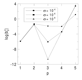
Figure 1: Magnitude of the memory function coefficient $b^{2}_{p}$ [Eq. (9)] as a function of the order $p$. These values were obtained for the Bernoulli map from a noisy correlation function for the observable $f(x)=x^{3}-\frac{1}{4}$; the parameter $\sigma$ gives the standard deviation of the gaussian random noise.

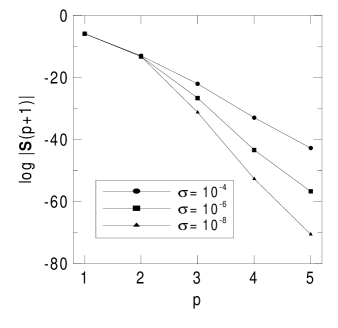
Figure 2: Magnitude of the determinant of the correlation matrix $\left|\mathbf{S}(p+1)\right|$ [Eq. (25)] as a function of the order $p$. These values were obtained for the Bernoulli map. Other details are as in Fig. 1.

In figures 1 and 2 we plot respectively, as a function of $p$, the magnitudes of $b^{2}_{p}$ and $\left|\mathbf{S}(p+1)\right|$ obtained from the noisy correlation function $C_{r}(n)$ for the Bernoulli map. We clearly observe in Fig. 1 that at the optimal order $p=p_{o}=3$ the coefficient $b^{2}_{p}$ is very sensitive to $\sigma$; the same sensitivity is observed in $\left|\mathbf{S}(p+1)\right|$ for $p\geq 3$ (Fig. 2). Besides, we observe that if the error in the correlation function is not small enough it may wash out completely the expected sharp decrease in both $b^{2}_{p}$ and $\left|\mathbf{S}(p+1)\right|$ at $p=p_{o}$; the determination of an optimal order would therefore require quite precise correlation values ($\sigma<10^{-4}$).

If instead one makes use of the self-consistent least-squares method described in Section IV, $p_{o}$ would be the order giving the minimum value of the error function $\xi$ defined in Eq. (32); in general, $p_{o}$ coincides with the maximum order $p$ for which self-consistency is achieved, i.e. for which the fixed point of Eq. (37) can be numerically reached. In the present case, for $\sigma<10^{-2}$ this occurs always at the correct value $p_{o}=3$, which indicates the ability of the least squares method to reduce the negative effects of the correlation noise.

Table 1: Resonance locations of the Bernoulli map. They were obtained from the solution of the eigenvalue problem in Section IV, which was set up for the autocorrelation function of the observable $f(x)=x^{3}-\frac{1}{4}$. The parameter $\sigma$ is the standard deviation of the gaussian randon noise added to the exact correlation values [see Eq. (44)], and $p$ is the order of the method, i.e. the expected number of resonances contributing to the correlation function; its correct value is $p=3$.

$\sigma$	$p$	$z_{1}$	$z_{2}$	$z_{3}$
	$2$	$0.4909$	$-03094$
$10^{-4}$	$3$	$0.4943$	$0.0881+0.3520i$	$0.0881-0.3520i$
	$4$	$0.5370$	$0.4733$	$-0.1207$
	$2$	$0.4909$	$-0.2891$
$10^{-6}$	$3$	$0.4998$	$0.2347$	$0.1379$
	$4$	$0.5001$	$0.2659$	$0.0949$
	$2$	$0.4909$	$-0.2889$
$10^{-8}$	$3$	$0.5000$	$0.2499$	$0.1251$
	$4$	$0.5000$	$0.2502$	$0.1251$

Let us now illustrate the effect of $\sigma$ in the resonance locations. In Table 1 we present the resonances derived from the solution of the eigenvalue problem defined in Section IV, which was set up for the noisy correlation function $C_{r}(n)$; different values for $\sigma$ and the order $p$ were used. We deduce from these results that the leading resonance $z_{1}$ is quite robust against noise and non optimal choices of the order $p$. The accurate location of other two resonances require, however, a better selection of $p$ and a more converged correlation function estimate; for instance, the $z_{2}$ and $z_{3}$ values obtained from the most noisy correlation ($\sigma=10^{-4}$) are completely wrong.

Table 2: Resonance locations of the Bernoulli map. They were obtained with the self-consistent least-square method described in Section IV. The optimal order $p=3$ given by this method was used. Other details are as in Table I.

$\sigma$	$z_{1}$	$z_{2}$	$z_{3}$
$10^{-4}$	$0.5003$	$0.2697$	$0.0850$
$10^{-6}$	$0.5000$	$0.2505$	$0.1243$
$10^{-8}$	$0.5000$	$0.2500$	$0.1250$

The resonance locations obtained from the self-consistent least-squares method are given in Table 2. As we already know, this method provides as the optimal order $p_{o}$ the correct value $p_{o}=3$. The method gives also significantly better resonance eigenvalues even in the case of large correlation noise ($\sigma=10^{-4}$), where the previous approach failed completely. In conclusion, when statistical errors are present in the estimated correlation function, of all the methods discussed in this work, the least-squares scheme provides the most accurate resonance values by reducing the negative effects of the correlation errors. In general, two factors increase the reliability of a resonance location obtained in this way: a larger stability and a larger contribution in the observable chosen.

The resonance generalized eigenvectors can be also determined from these schemes. For the Bernoulli map the calculated right eigenvectors are approximations to the Bernoulli polynomials participating in the observable chosen; a better estimate of the eigenvalue gives a better approximation to the corresponding Bernoulli polynomial. However the left eigenvectors provided by these schemes are wrong representation of the true ones. The reason for such an incorrect result may lie in the observable chosen and in the very different nature of the exact left and right generalized eigenvectors: while the right ones are functions, the left ones are distributions; this asymmetry is a consequence of the non-invertibility of the map. Therefore, the expansion of our observable (a polynomial) in the right eigenvector (Bernoulli polynomial) has a finite number of terms while this number is infinite if such expansion is performed in the left ones. When these two numbers are different, as in our case, we know from the final discussion in Section IV that the present schemes will provide a representation for the states and resonances of the shorter expansion.

As a second example we will consider the standard map chirikov

$$x_{n+1} = x_{n}+y_{n},$$

$$y_{n+1} = y_{n}+\frac{K}{2\pi}\sin\left(2\pi x_{n+1}\right),\quad(\textrm{mod }1)$$ (45)

This map is area-preserving and invertible. While for $K=0$ it is integrable, for $K\neq 0$ presents chaotic phase space regions which become more extensive as $K$ increases. The system follows the route to chaos known as overlapping resonances chirikov ; note . We take the value $K=10$ in our calculations.

The exact knowledge of the PR resonances is not generally possible for this system. Blum and Agam blum proposed a variational approach to locate the four leading ones, which as we are already aware, is a $p=4$ implementation of the eigenvalue problem derived in this work. For comparison, we will take the observable chosen by these authors, i.e.

$$f(x,y)=\exp\left(i2\pi x\right),$$ (46)

whose autocorrelation function may be decomposed as the sum of the autocorrelation functions for $\cos 2\pi x$ ($C_{c}$) and $\sin 2\pi x$ ($C_{s}$)

$$C(n)=C_{c}(n)+C_{s}(n).$$ (47)

This decomposition is possible because the standard map has an inversion symmetry with respect to the point $(x=\frac{1}{2},\;y=\frac{1}{2})$; therefore, the generalized eigenvectors are either symmetric or antisymmetric under this transformation. The symmetric ones will participate in $C_{c}(n)$, while the antisymmetric ones will do in $C_{s}(n)$.

Table 3: Locations of leading resonances in the standard map for $K=10$. The first two lines correspond respectively to $C_{c}(n)$ and $C_{s}(n)$ autocorrelation functions. The resonances were obtained from these correlation functions using the self-consistent least-squares scheme. The bottom line gives the four values obtained by Blum and Agam blum from their $p=4$ variational approach

$f$		$z_{i}$
$\cos(2\pi x)$	$0.672$	$-0.030\pm 0.702i$	$0.332\pm 0.503i$
$\sin(2\pi x)$	$-0.715$	$0.150\pm 0.592i$	$-0.119\pm 0.553i$
$e^{i2\pi x}$ blum	$0.515$	$-0.494$	$-0.003\pm 0.505i$

Both $C_{c}(n)$ and $C_{s}(n)$ have been determined here from the system orbits with an uncertainty $\sigma<10^{-5}$. We have proceeded next to implement the self-consistent least-squares method of Section IV to find the leading PR resonances. As a first result we obtain for the optimal order the values $p_{o}=9$ from $C_{c}(n)$, and $p_{o}=8$ from $C_{s}(n)$. The location of the leading resonances is given in Table 3. Since the two correlation functions do not have common eigenvalues, the total optimal order corresponding to the initial observable in Eq. (46) is $p_{o}=17$; this number is much larger than the value $p=4$ used by Blum and Agam. If we take this smaller order to solve the general eigenvalue problem, the locations that we obtain for the the four resonances coincide exactly with those found by these authors; they are also included in Table 3. However, if we increase $p$ just by one these values change significantly, which means that they are not properly converged.

The corresponding left and right generalized eigenvectors are expected to be complicated distributions. In this case, as we have discussed in Section IV, the eigenfunctions derived from our numerical approach are smooth representations of them. In Fig. 3 we present the numerical left and right eigenfunctions associated with each of the two leading resonances of the standard map; the first pair is symmetric and the second one antisymmetric under the inversion transformation. To better illustrate the intricate structure we have selected small regions of the available phase space.

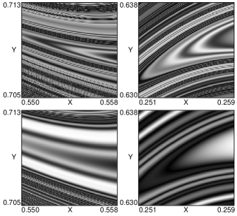
Figure 3: Structure of the right (right panels) and left (left panels) generalized eigenvectors corresponding to the real resonances $z_{i}=0.672$ (top) and $z_{i}=-0.715$ (bottom) in the standard map ($K=10$). The eigenvectors in the top panels are symmetric under the inversion transformation and participate in the cosine correlation function $C_{c}$; those in the bottom panels are antisymmetric and participate in the sine correlation function $C_{s}$. To better illustrate the intricate structure we have selected small regions of the available phase space. Absolute magnitudes are represented, with higher values corresponding to brighter regions.

VI Summary

Among the schemes followed in the literature to locate the leading Pollicott-Ruelle resonances of the Perron-Frobenius operator in chaotic dynamical systems, there are a few examples of remarkable simplicity, which involve either the use use of Padé approximants to perform the analytical continuation of the spectral density functions isola ; baladi , or the diagonalization of small dynamically adapted eigenvalue problems blum . In an attempt to provide a theoretical support to these methods, we have analyzed their connection with other numerical schemes used in different contexts. A first category of such schemes includes the memory function techniques memory used in the general theory of relaxation, and the methods related to this approach such as those based on the use of continued fractions and Padé approximants. In a second category we have also considered the methods of the filter diagonalization approach neuhauser ; taylor , which is a particular formulation of the harmonic inversion of a time signal as an eigenvalue problem.

The analysis of these schemes led us to a theoretical framework in which all them become equivalent formulations of the same problem: the location of the leading resonances contributing to a give time correlation function. The most convenient of these formulations is as an eigenvalue problem from which one can obtain not only the poles, i.e. the resonance locations, but also a smooth representation of the generalized eigenvectors. Besides, we have proved that all these procedures are also particular linear formulations of the non-linear numerical problem known as interpolation by exponentials baladi ; henrici . This connection has provided us with new tools to perform a better analysis of issues such as convergence and numerical stability. From such analysis improved schemes may be designed, as the one that we have proposed based on a least-squares fit.

We have illustrated the use of this class of methods in two chaotic maps: the Bernoulli map and the standard map. In the first example the nature of the right eigenvectors, which are known to be the Bernoulli polynomials, allows for finite expansion of certain observables like the one chosen for illustration. Then an accurate enough correlation function provides good approximations to the PR resonances and their corresponding right eigenvectors. The least squares method improves significantly these results in the case of less accurate correlation values.

In the standard map, for which the exact knowledge of the PR resonances is not generally possible, the more elaborated least squares method provides resonances values which appear to be significantly more converged than previous results blum . Nice smooth representations of the eigendistributions are also obtained. These indicate the relevant phase space regions involved in the dynamics.

- (1) M. Pollicott, Invent. Math. 81, 413 (1985); 85, 147 (1986).
- (2) D. Ruelle, Phys. Rev. Lett. 56, 405 (1986); J. Differ. Geom. 25, 99 (1987).
- (3) P. Gaspard, Chaos, Scattering and Statistical Mechanics, (Cambridge University Press, Cambridge, 1998).
- (4) B.L. Altshuler and B.I. Shklovskii, JETP 64, 127 (1986).
- (5) B.A. Muzykantskii and D.E. Khmelnitskii, JETP Lett. 62, 76 (1995); A.V. Andreev, O. Agam, B.D. Simons and B.L. Altshuler, Phys. Rev. Lett. 76, 3947 (1996).
- (6) J.M. Gomez Llorente, H.S. Taylor, and E. Pollak, Phys. Rev. Lett. 62, 2096 (1989); J.M. Gomez Llorente and H.S. Taylor, Phys. Rev. A 41, 697 (1990).
- (7) G. Blum and O. Agam, Phys. Rev. E 62, 1977 (2000).
- (8) J. Weber, F. Haake, and P. Seba, Phys. Rev. Lett. 85, 3620 (2000).
- (9) P. Gaspard and D. Alonso Ramírez, Phys. Rev. A 45, 8383 (1992).
- (10) F. Christiansen, G. Paladin and H.H. Rugh, Phys. Rev. Lett. 65, 2087 (1990).
- (11) S. Isola, Commun. Math. Phys. 116, 343 (1988).
- (12) V. Baladi, J.-P. Eckmann and D. Ruelle, Nonlinearity 2, 119 (1989).
- (13) G. Grosso and G. Pastori Parravicini, Adv. Chem. Phys. 62, 133 (1985).
- (14) M.R. Wall and D. Neuhauser, J. Chem. Phys. 102, 8011 (1995).
- (15) V.A. Mandelshtam and H.S. Taylor, Phys. Rev. Lett. 78, 3274 (1997).
- (16) P. Henrici, Applied and Computational Complex Analysis (Wiley, New York, 1974).
- (17) R. Zwanzig, J. Chem. Phys. 33, 1338 (1960).
- (18) H. Mori, Prog. Theor. Phys. 33, 423 (1965); 34, 399 (1965).
- (19) G. Grosso and G. Pastori Parravicini, Adv. Chem. Phys. 81, 133 (1985).
- (20) E. Narevicius, D. Neuhauser, H.J. Korsch, N. Moiseyev, Chem. Phys. Lett. 276, 250 (1997); V.A. Mandelshtam, J. Chem. Phys. 108, 9999 (1998); K. Weibert, J. Main, and G. Wunner, Eur. Phys. J. D 12, 381 (2000).
- (21) S.L. Marple, Jr., Digital Spectral Analysis with Applications (Prentice-Hall, London, 1987).
- (22) B.V. Chirikov, Phys. Reports 52, 263 (1979).
- (23) The term resonance here does not mean PR resonance but dynamical resonance between torus frequencies.