Statistics and Characteristics of Spatio-Temporally
Rare Intense Events in Complex Ginzburg-Landau Models

Abstract

We study the statistics and characteristics of rare intense events in two types of two dimensional Complex Ginzburg-Landau (CGL) equation based models. Our numerical simulations show finite amplitude collapse-like solutions which approach the infinite amplitude solutions of the nonlinear Schrödinger (NLS) equation in an appropriate parameter regime. We also determine the probability distribution function (PDF) of the amplitude of the CGL solutions, which is found to be approximately described by a stretched exponential distribution, $P(|A|)\approx e^{-|A|^{\eta}}$, where $\eta<1$. This non-Gaussian PDF is explained by the nonlinear characteristics of individual bursts combined with the statistics of bursts. Our results suggest a general picture in which an incoherent background of weakly interacting waves, occasionally, ‘by chance’, initiates intense, coherent, self-reinforcing, highly nonlinear events.

I Introduction

Many spatio-temporal dynamical systems show rare intense events. One example is that of large height rogue ocean waves Osborne1 . Another example occurs in recent experiments on parametrically forced surface waves on water in which high spikes (bursts) on the free surface form intermittently in space and time Lathrop . Other diverse physical examples also exist (e.g., tornados, large earthquakes, etc.). The characteristic feature of rare intense events is an enhanced tail in the event size probability distribution function. Here, by enhanced we mean that the event size probability distribution function approached zero with increasing event size much more slowly than is the case for a Gaussian distribution. Thus these events, although rare, can be much more common than an expectation based on Gaussian statistics would indicate. The central limit theorem implies Gaussian behavior for a quantity that results from the linear superposition of many random independent contributions. Non-Gaussian tail behavior can result from strong nonlinearity of the events, and enhancement of the event size tail might be expected if large amplitudes are nonlinearly self-reinforcing. Such nonlinear self-reinforcements is present in the nonlinear Schrödinger (NLS) equation. In particular, the two dimensional NLS equation,

$$\frac{\partial A}{\partial t}=-i\alpha|A|^{2}A-i\beta\bigtriangledown^{2}A.$$ (1)

exhibits “collapse” when the coefficients $\alpha$ and $\beta$ have the same sign Bartuccelli . In a collapsing NLS solution the complex field approaches infinity at some point in space, and this singularity occurs at finite time. The NLS is conservative in that it can be derived from a Hamiltonian, $\partial A/\partial t=-i\delta H/\delta A^{*}$, where $H[A,A^{*}]=\frac{1}{2}\int[\alpha|A|^{4}+\beta|\bigtriangledown A|^{2}]d{\bf x}$. In the case of nonconservative dynamics, inclusion of lowest order dissipation and instability terms leads to the complex Ginzburg-Landau (CGL) equation Levermore . The CGL equation has been studied as a model for such diverse situation as chemical reaction Chemical , Poiseuille flow Poiseuille , Rayleigh-Bérnard convection Rayleigh , and Taylor-Couette flow Taylor . In the limit of zero dissipation/instability the CGL equation approaches the NLS equation. For small nonzero dissipation/instability, the CGL equation displays a solution similar to the NLS collapse solution, but with a large finite (rather than infinite) amplitude at the collapse time Bartuccelli . Furthermore, over a sufficiently large spatial domain, these events occur intermittently in space and time. Thus, in this parameter regime, the CGL equation may be considered as a model for the occurrence of rare intense events.

In this paper we study the statistics and characteristics of rare intense events in a two-dimensional CGL-based model. The probability distribution function (PDF) of the amplitude of the solutions is observed to be non-Gaussian in our numerical experiments. This non-Gaussian PDF is explained by the nonlinear characteristics of individual bursts combined with the statistics of bursts. The model equation we investigate is

$$\frac{\partial A}{\partial t} = \pm A-(1+i\alpha)|A|^{2}A+(1-i\beta)\bigtriangledown^{2}A$$ (2)

$$+(\delta_{r}+i\delta_{i})A^{*},$$

where $(\delta_{r}+i\delta_{i})A^{*}$ is a parametric forcing term Park . We will consider two cases: one without parametric forcing ($\delta_{r}=\delta_{i}=0$) in which case the plus sign is chosen in front of the first term on the right-hand side of (2) (Eq. (2) is then the usual CGL equation), and one with parametric forcing, in which case the minus sign is chosen. As previously discussed, we choose our parameters so that our model, Eq. (2), is formally close to the NLS equation (1). That is, we take $\alpha,\beta\gg 1,\delta_{r},\delta_{i}$, and for our numerical solutions we will restrict attention to the case $\alpha=\beta$. Note that the coefficient $\pm 1$ for the first term, as well as the ones in $(1+i\alpha)$ and $(1+i\beta)$ represent no loss of generality, since these can be obtained by suitable scaling of the time($t$), the dependent variable($A$), and the spatial variable(${\bf x}$). In Section II, we discuss the amplitude statistics of our two-dimensional CGL models with and without the parametric forcing term. We find that the PDFs are approximately described by a stretched exponential distribution, $P(|A|)\approx\exp(-|A|^{\eta})$, where $\eta$ is less than 1. In Section III, we investigate the characteristics of individual bursts. We compare our numerical CGL results with known collapse solutions of the NLS equation. The maximum amplitude obtained by many bursts (or the “event size” statistics) is discussed in Section IV. Section V presents further discussion and conclusions.

Our results lead us to the following picture for the occurrence of rare intense events in our system. Linear instability and nonlinear wave saturation lead to an incoherent background of small amplitude waves. This background is responsible for the observed small $|A|$ Gaussian behavior of our probability distribution functions. When, by chance, the weakly interacting waves locally superpose to create conditions enabling nonlinear, coherent self-reinforce, a localized, collapse-like event is initiated. Collapse takes over, promoting large, rapid growth and spiking of $A$. This is followed by a burn-out phase in which the energy in rapidly dissipated due to the generation of small scale structure by the spike. We believe that elements of the above general picture may be relevant to a variety of physical situations where rare intense events occur (e.g., the parametrically driven water wave experiments in Ref. Lathrop ).

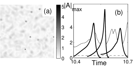
Figure 1: Solutions of the CGL model. (a) Snapshot of the amplitude $|A|$ for $L=20\pi$, $\alpha=\beta=30$, $\Delta t=10^{-5},\delta_{r}=\delta_{i}=0$ and a $256\times 256$ grid. (b) Amplitude profile versus time. Solid line indicates $|A|_{max}$ of the whole system, while thick solid lines indicate maximum amplitude of the localized events(”bursts”). The dashed line indicates the average amplitude of $|A|$ over the whole system $|A|_{avg}\sim 0.3$.

II Amplitude Statistics

II.1 2D model without a parametric force ($\delta_{r}=\delta_{i}=0$)

We first consider Eq.(2) with $\delta_{r}=\delta_{i}=0$ and with the plus sign in the first term on the right hand side of the equation. Figure 1(a) shows a representation of $|A({\bf x},t)|$ [from numerical solution of Eq. (2)] at a fixed instant $t$, where large values are indicated by darker grey shades. As a function of time, the localized dark shades occur in an seemingly random manner, become darker (i.e., increase their amplitude) and then go away (become light). Furthermore, the maximum amplitudes also display apparent randomness. [see Fig. 1(b)]. As shown in the next section (Sec. III), although the occurrence of these intense events is apparently erratic in time and space, individually these events are highly coherent. In this section, we will study the statistical properties of $A({\bf x},t)$.

Our numerical solutions of (2) employ periodic boundary conditions on a $256\times 256$ grid. We choose the parameters, $\alpha$ and $\beta$, large enough ($\alpha=\beta=30$) so that the solutions of our model are close to solutions of the NLS equation. We choose the time step small enough to satisfy the condition for unconditional stability of our second-order accurate time integration($\Delta t=10^{-5}$). We use random initial condition (at $t=0$, we generate random values for amplitudes and phases at each grid point). Localized structures, ”bursts”, develop very rapidly and occur throughout the spatial domain. The typical life time of a burst ($\delta t$) is approximately 0.2 time units. The maximum amplitudes of bursts are different for different burst events.

Imagining that we choose a space-time point $({\bf x},t)$ at random, we now consider the probability distribution functions for $|A|$ (the magnitude of $A$), $A_{r}=Re[A]$ (the real part of $A$), and $A_{i}=Im[A]$ (the imaginary part of $A$). We denote these distribution functions $P(|A|),P_{r}(A_{r}),P_{i}(A_{i})$, and we compute them via histogram approximations using the values of $|A|,A_{r},$ and $A_{i}$ from each of the $256\times 256$ grid points at many time frames footnote . We find that these distributions are independent of the periodicity length $L$ used in the computation as long as it is sufficiently large compared to the spatial size of a burst, but is not so large that spatial resolution on our $256\times 256$ grid becomes problematic. In our computations of $P,P_{r}$ and $P_{i}$, we choose $L=20\pi$.

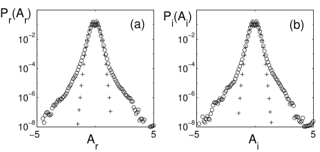
Figure 2: Probability distribution functions obtained from numerical solution of Eq.(2) using the same parameters as in Fig. 1. The circles are data for $P_{r}$ and $P_{i}$, while the pluses are the probability distributions $P_{r}^{\prime}$ and $P_{i}^{\prime}$ obtained from the phase randomized amplitude.

Figures 2 show the numerically computed probability distributions $P_{r}(A_{r})$ [Fig. 2(a)] and $P_{i}(A_{i})$ [Fig. 2(b)] plotted as open circles. Since Eq. (2) with $\delta_{r}=\delta_{i}=0$ is invariant to the transformation $A\rightarrow A\exp(i\phi)$ (where $\phi$ is an arbitrary constant), we expect the distribution $P_{r}$ and $P_{i}$ to be the same to within the statistical accuracy of their determinations. This is born out by Figs. 2. In order to highlight the essential role that nonlinearity plays in determining these distribution functions, we have also computed them after randomizing the phases of each Fourier component. That is, representing $A({\bf x},t)$ as

$$A({\bf x},t)=\sum_{{\bf k}}a_{{\bf k}}(t)\exp(i{\bf k}\cdot{\bf r}),$$ (3)

where ${\bf k}=(2m\pi/L,2n\pi/L)$, we form a new amplitude, $A^{\prime}({\bf x},t)$ as

$$A^{\prime}({\bf x},t)=\sum_{{\bf k}}a_{{\bf k}}(t)\exp(i{\bf k}\cdot{\bf r}+i\theta_{{\bf k}}),$$ (4)

where for each ${\bf k}$, the angle $\theta_{{\bf k}}$ is chosen randomly with uniform probability density in $[0,2\pi]$. The probability distribution functions for the real and imaginary parts of the randomized amplitudes $A^{\prime}$ are shown as pluses in Figs. 2. Note that by construction, $A$ and $A^{\prime}$ have identical wavenumber power spectra. Due to the random phases, $A^{\prime}$ at any given point $\bf{x}$ can be viewed as a sum of many independent random numbers (the Fourier components). Hence the $P_{r}$ and $P_{i}$ distributions are expected to be Gaussian, $\log P_{r,i}\sim[(const.)-(const.)A_{r,i}^{2}]$. This is confirmed by the semi-log plots of Figs. 2, where the data plotted as pluses can be well-fit by parabolae.

The above comparisons with the phase randomized variable $A^{\prime}$ are motivated by imagining the hypothetical situation where the amplitude is formed by the superposition of many noninteracting linear plane waves. In that case we would have an amplitude field of form

$$\sum_{{\bf k}}b_{{\bf k}}(t)\exp(i{\bf k}\cdot{\bf r}+i\omega_{{\bf k}}t).$$ (5)

Because $\omega_{{\bf k}}$ is different for different ${\bf k}$, the phases become uncorrelated for sufficiently large time $t$.

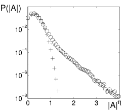
Figure 3: Probability distribution functions before randomizing the phases of the solutions (o) and after randomizing the phases (+). Note the horizontal axis is $|A|^{\eta}$, where the exponent $\eta=0.8$ is chosen to yield approximately linear dependence of $\log[P(|A|)]$ on $|A|^{\eta}$ for large values of $|A|$.

Comparing the data from $A$ and $A^{\prime}$ in Figs. 2, for small values of $A_{r}$ and $A_{i}$, the PDFs are nearly Gaussian. This can be attributed to near linear behavior of small amplitude waves. On the other hand, for the tails of the distributions, we note substantial enhancement relative to the Gaussian distributions. These must be due to coherent phase correlations resulting from nonlinear interaction of different wavenumber components of $A$. Such phase coherence is implied by the observed coherent localized burst structures.

Figure 3 shows the numerically obtained distribution $P(|A|)$ plotted as circles and the probability distribution for the phase randomized amplitude $|A^{\prime}|$ plotted as pluses. Again, the enhancement of the large amplitude tail is evident. Note that the vertical axis in Fig. 3 is logarithmic, while the horizontal axis is $|A|^{\eta}$. Here we choose the power $\eta=0.8$ so that the large $|A|$ data in this plot are most nearly fit by a straight line. That is, we attempt to fit $P(|A|)$ using a stretched exponential. The slope of the dashed straight line in the figure is chosen to match the large $|A|$ data. Thus, over the range of $|A|$ accessible to over numerical experiment, we find that the enhanced large $|A|$ tail probability density is roughly fit by a stretched exponential,

$$P(|A|)\sim\exp(-\zeta|A|^{0.8}).$$ (6)

II.2 2D model with parametric forcing ($\delta_{r},\delta_{i}\neq 0$)

We now report similar results for the case of parametric forcing, Eq. (2) with $\delta_{r},\delta_{i}\neq 0$ and the minus sign chosen in the first term on the right side of (2). In this case, instability of small amplitude waves is caused by the parametric forcing (nonzero $\delta_{r,i}$) and the $-A$ term represents a linear wavenumber independent damping. This model for parametric forcing was introduced Corellet and has been used to model various situations. One such situation is that of periodically forced chemical reactions Hagberg . Our motivation for considering this model is the Faraday experiments on strong parametric forcing of surface water waves in Ref. Lathrop . In that work intermittent formation of large localized surface perturbations results in splash and droplet formation.

Parameters for our numerical simulations are the same as in Sec. IIA except that now $\delta_{r}=\delta_{i}=5$. Again coherent localized structures, ”bursts”, develop rapidly and occur intermittently throughout the spatial domain, Fig. 4(a). As in Sec. IIA, the typical life time of a burst is less than 0.2 time units, and the maximum amplitudes of bursts are different for different bursts.

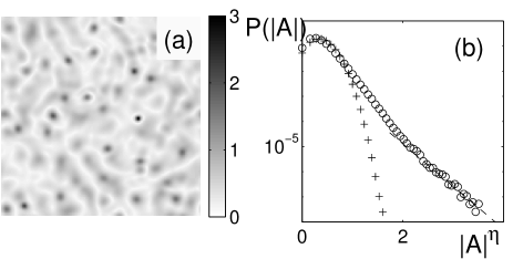
Figure 4: Solutions of the model with parametric forcing. (a) snapshot of $|A|$. Dark regions have high amplitudes. (b) $P(|A|)$ versus $|A|^{\eta}$, where $\eta=0.8$. (See captions in Fig. 3.)

The PDF, $P(|A|)$ again shows a stretched exponential tail with exponent $\eta=0.8$, Fig. 4(b). The circles in Figs. 5 show the PDFs of the real and imaginary parts of $A$, while the pluses are data for the PDFs after randomizing the phase. The shape of the PDFs around the central part are nearly Gaussian. In contrast, at large amplitude the PDFs are significantly non-Gaussian. A major difference with the case $\delta_{r}=\delta_{i}=0$ is that, with parametric forcing, the model is not invariant to $A\rightarrow Ae^{i\phi}$, and thus $P_{r}$ and $P_{i}$ may be expected to evidence differences not present for $\delta_{r}=\delta_{i}=0$. This is seen to be the case in Figs. 5.

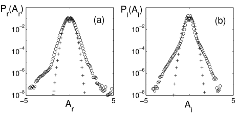
Figure 5: $P_{r}(A_{r})$ and $P_{i}(A_{i})$ with parametric forcing. The numerical parameters are the same as those for Fig. 4. The circles are PDFs for $A_{r}$ and $A_{i}$ before randomizing the phases of the solutions, while pluses are PDFs after randomizing the phases.

III Characteristics of Individual Burst Events

Solutions of the CGL equation with large $\alpha$ and $\beta$ may be expected to have features in common with solutions of the NLS equation. It is known that the NLS equation yields localized events which develop finite time singularities where the amplitude becomes infinite  Levermore . While it is difficult to understand the dynamics of the solutions of CGL equation from direct rigorous analysis, the solutions of the NLS equation are relatively well understood. Thus, we analyze the dynamics of individual CGL bursts guided by the known localized self-similar collapsing solution of the NLS equation.

The NLS equation has a special solution Fibich of the form

$$A=e^{i\theta t}R(r),~{}~{}~{}~{}r=\sqrt{x^{2}+y^{2}},$$ (7)

where the radial function $R(r)$ satisfies

$$\left(\frac{\partial^{2}}{\partial r^{2}}+\frac{1}{r}\frac{\partial}{\partial r}\right)R-\xi R+R^{3}=0,$$ (8)

$$~{}~{}\left|\frac{\partial R}{\partial r}\right|_{r=0}=0,~{}~{}R(\infty)=0,$$

where $\alpha=\beta$, $\xi=\theta/\beta$ . Since (1) is invariant under the scaling transformation Lemesurier ,

$$A({\bf x},t)\longrightarrow L(t)^{-1}A({\bf\kappa},\tau){\rm e}^{iL\dot{L}|{\bf\kappa}|^{2}/4},$$ (9)

where $L(t)$ tends to zero as $t^{*}\longrightarrow t$, $t<t^{*}$ and

$${\bf\kappa}=\frac{{\bf x}}{L(t)},~{}~{}~{}~{}\tau=\int_{0}^{t}\frac{1}{L^{2}(s)}ds,$$ (10)

a family of collapsing solutions of the NLS is given by the rescaled solution of Eq. (8).

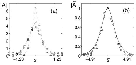
Figure 6: Self-similar bursts. (a) Enlarged plots of a burst at $t_{1}(\bigcirc)=10.448,$ at grid point $(x,y)=(15.2,22.1),$ and $t_{2}(\triangle)=10.530,$ at grid point $(51.1,25.5),$ and $t_{3}(\square)=10.644$ at grid point $(57.4,38.8)$. (b) Scaled profiles, where $|\tilde{A}|=|A|/L$, $\tilde{x}=x/L$, and $L=|A|_{max}$ at $t_{1}$, $t_{2}$, and $t_{3}$. The solid line represents the radial solution of Eq. (8).

With these considerations, we test the expected approximate self-similarity of individual bursts observed in our numerical solutions of Eq. (2). We consider three typical bursts that occur at different times and spatial positions. In particular, we choose these three as the three dark regions in Fig. 1(a) whose spatial maxima have the time dependences shown as thick solid lines in Fig. 1(b).

In Fig. 6(a) we plot the $x$-dependence of $|A|$ at constant $y$ for each of these bursts at the time that they reach their maximum amplitude (the positions in $x$ of the maxima have been shifted to $x=0$ and the constant $y$ value for each is at the location of $|A|_{max}$). Note that, when they reach their maxima, the three bursts have different amplitudes and width. We rescale the amplitude and spatial coordinate as suggested by (9) and (10), $|\tilde{A}|=|A|/L$ and $\tilde{x}=x/L$, and we take $L=|A|_{max}$ (which normalizes $|\tilde{A}|_{max}$ to one). The resulting data are plotted in Fig. 6(b) along with the solution of Eq. (8). [We again rescale $R(r)$ using (9) and (10), and we note that, after this rescaling, the result is independent of the value of $\xi=0.1$ in Eq. (8).] The three burst profiles show evidence of collapsing onto the theoretical radial solution.

Now, we consider the time dependence of a single burst. We select the burst at the grid point $(x,y)=(51.1,25.5)$ (see caption to Fig. 6) and investigate the evolution of its shape and height. We display profiles of the burst at 5 different times in Fig. 7(a). Rescaling each profile using Eq. (9) and Eq. (10), and defining $L$ in the same way as before, the four profiles at the first four times approximately collapse onto the radial solution of (8) as shown in Fig. 7(b). When the burst reaches its maximum amplitude, the amplitude at some distance away from the center becomes zero (see the amplitude profile at $t=t_{3}$). After that, the center decays very rapidly (see the amplitude profile at $t=t_{5}$). (Note that in this section and the next section, we present numerical results for (2) with $\delta_{r}=\delta_{i}=0$. However, we have also verified that the CGL model with parametric forcing also has similar self similarity properties.)

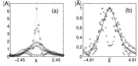
Figure 7: Self-similarity of single burst. (a) Enlarged plots of a burst at $t_{1}(\bigcirc)=10.50$, $t_{2}(\square)=10.52$, $t_{3}(\triangle)=10.53$, $t_{4}(\diamond)=10.54$, and $t_{5}(\times)=10.55$. (b) Scaled profiles, where $|\tilde{A}|=|A|/L$, $\tilde{x}=x/L$, and $L=|A(r)|_{max}$ at $t_{1},t_{2},t_{3}$, and $t_{4}$. The solid line represents the solution of Eq. (8).

IV Statistics of Bursts

The self similar properties of bursts implies that the solutions of the CGL model consist of self-similar bursts of various maximum heights. Thus, we expect that the enhanced tail (the deviation from the Gaussian distribution) of the amplitude probability distribution $P(|A|)$ can be understood by the statistics of bursts. In particular, we consider $g(h)$, the frequency of bursts which have maximum height $h$, and a distribution $P_{j}(|A|)$ defined for an individual burst (burst $j$), as follows.

We define the time interval for each burst as the time between when its peak value exceeds $2|A|_{avg}$ and when its peak value drops below $2|A|_{avg}$ [typically the time duration of a burst is less than $0.2$, see Fig. 1(b)]. Here $|A|_{avg}$ is the space average of $|A|$ over the entire spatial grid of the simulation at each time $t$ [$|A|_{avg}$ is approximately constant at about $0.3$ over all time steps in the simulation, see the dashed line in Fig. 1(b)]. Consistent with the observation that a typical burst has radial symmetry, we define the domain of the burst to be a circular region of radius $r_{eff}$ centered at the burst maximum, where $r_{eff}$ is the maximum radius of a circle such that the average of $|A|$ over the perimeter of the circle is greater than $2|A|_{avg}$ (typically, $1.23\leq r_{eff}\leq 4.91$). In Fig. 8(a) we show the distribution $P_{j}(|A|)$ for the three bursts in Fig. 1(b) (thick solid lines). The first burst ($j=1$) has $h=4.52$ and is plotted as the open circles in Fig. 8(a); the second burst ($j=2$) has $h=6.31$ and is plotted as the open triangles; and the third burst ($j=3$) has $h=3.85$ and is plotted as the open squares. These distributions are obtained from histograms of the values of $|A|$ at grid points in the domains and time steps in the duration of each of these bursts. We obtain $g(h)$ by counting the number of bursts which have maximum heights between $h$ and $h+\Delta h$, where $\Delta h=0.2$ [see Fig. 8(b)]. (In Fig. 8(a) $P_{j}(|A|)$ is not plotted for $|A|<2|A|_{avg}$, since, by our procedure this range lacks meaning, and since we are interested in the behavior at large values of $|A|$.) We note that the $P_{j}(|A|)$ in Fig. 8 all approximately coincide for $|A|<h$. Thus the only characteristic of the bursts on which $P_{j}(|A|)$ depends is the maximum burst amplitude $h$ at which $P_{j}(|A|)$ goes to zero. To incorporate this fact, we replace $P_{j}(|A|)$ by the notation $P_{h}(|A|)$.

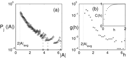
Figure 8: Statistics of localized events(”bursts”). (a) $P_{h_{j}}(|A|)$ at three different times: $t_{1}(\bigcirc)=10.448$ and $h=4.52$, $t_{2}(\triangle)=89.0$ and $h=6.31$, and $t_{3}(\square)=94.0$ and $h=3.85$. (b) The frequency of bursts which have maximum height $h$, $g(h)$. The inset indicates $C(h)$ versus $h$ defined in Eq. (13).

The above suggests that $P(|A|)$ can be obtained from the following approximation Iwasaki

$$P(|A|)\sim\int_{0}^{\infty}g(h)P_{h}(|A|)dh,$$ (11)

where $P_{h}(|A|)$ is a probability distribution of a single burst whose temporal maximum amplitude is $h$. Since $P_{h}(|A|)$ vanishes for $|A|>h$ and because the $P_{h}(|A|)$ approximately coincide for $|A|<h$ [see Fig. 8(a)], we approximate $P_{h}(|A|)$ as

$$P_{h}(|A|) \sim C^{-1}(h)\theta(h-|A|)P_{*}(|A|),$$ (12)

$$C(h) = \int_{0}^{h}P_{*}(|A|)d|A|,$$ (13)

where $C(h)$ is a normalization factor [$C(h)\sim 1$, when $h>1$; see the inset on Fig. 8(b)], $\theta(h-|A|)$ is a step function, and $P_{*}$ is the distribution that we numerically compute at the largest value of $h$ that we considered ($h_{max}=6.31$). Using (11) and (13), we can further approximate $P(|A|)$ as

$$P(|A|) \sim \int_{0}^{\infty}C^{-1}(h)\theta(h-|A|)g(h)P_{*}(|A|)dh$$ (14)

$$\sim P_{*}(|A|)\int_{|A|}^{\infty}C^{-1}(h)g(h)dh.$$

(The integral in (14) is the cumulative frequency of bursts which have maximum height greater than $|A|$.)

Figures 8 show the numerically obtained $g(h)$ and $P_{*}(|A|)$. Inserting $P_{*}(|A|)$ into Eq.(13) and Eq.(14), we obtain the prediction for $P(|A|)$ plotted as pluses in Fig. 9 for $|A|>2|A|_{avg}$. This appears to agree well with the $P(|A|)$ obtained from our numerical solutions of (2) (open circles). (Note that we shift the predicted $P(|A|)$ (pluses) to the $P(|A|)$ (open circles) obtained from (2) after removing data points for $|A|<2|A|_{avg}$.)

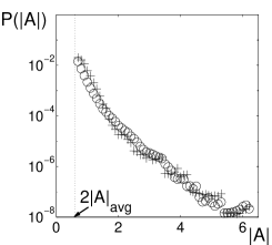
Figure 9: $P(|A|)$ versus $|A|$. Circles represent $P(|A|)$ obtained directly from our numerical solutions of (2), while pluses represent $P(|A|)$ obtained using $P_{*}(|A|)$ and $g(h)$ from Fig. 8, and Eqs. (11)-(14).

V Conclusion

We find that the large $A$ behavior of the PDF obtained from our CGL solutions is approximately described by a stretched exponential form, $P(|A|)\approx e^{-|A|^{\eta}}$, where $\eta<1$. In addition, for small $A$, $P_{r}(A_{r})$ and $P_{i}(A_{i})$ are approximately Gaussian, as is the case for a random linear superposition of waves. We also observe the self similar properties of individual bursts, which allow us to consider the large amplitude behavior of our CGL solutions as composites of coherent self similar bursts. Based on this we explain the observed non-Gaussian $P(|A|)$ using the nonlinear characteristics of individual bursts $P_{h}(|A|)$ combined with the statistics of burst occurrences $g(h)$.

These results lead us to conjecture the following picture of rare intense events in our model. Linear instability leads to a background of relatively low amplitude waves that are weakly interacting and result in a random-like, incoherent background and low $|A|$ Gaussian behavior of $P_{r}(A_{r})$ and $P_{i}(A_{i})$. When, by chance, this incoherent behavior results in local conditions conductive to burst formation, nonlinear, coherent, self-reinforcing collapse takes over and promotes a large growth and spiking of $A$. We believe that this general mechanism may be operative in a variety of physical situations in which rare intense events occur (e.g., the water wave experiments of Ref. Lathrop ).

We thank D. P. Lathrop for initial discussion and for attracting our attention to the subject of rare intense events. We thank P. N. Guzdar for his advice on numerics. This work was supported by the Office of Naval Research (Physics) and by the National Science Foundation (PHY0098632).

References

- (1) A. R. Osborne, M. Onorato, and M. Serio, Phys. Lett. A 275 , 386(2000).
- (2) J. E. Hogrefe, et al., Physica D 123 183(1998); B. W. Zeff, et al., Nature 403 401(2000).
- (3) M. Bartuccelli, et al., Physica D 44 , 421(1990). They draw a phase diagram figures for NLS equation (Fig. 1) and CGL equation (Fig. 2).
- (4) C. D. Levermore and M. Oliver, Lect. Appl. Math. 31 141(1996).
- (5) Y. Kuramoto, Chemical Oscillations, Waves and Turbulence , Series in Synergetics 19 , Springer, New York, 1984.
- (6) K. Stewartson and J.T. Stuart, J. Fluid Mech. 48 , 529(1971).
- (7) A.C. Newell and J.A. Whitehead, J. Fluid Mech. 38 , 279(1969).
- (8) G. Ahlers and D.S. Cannell, Phys. Rev. Lett. 50 , 1583(1983).
- (9) H.-K. Park, Phys. Rev. Lett. 86 1130(2000); also see the references therein.
- (10) is to be contrasted with the probability distribution of a single burst amplitude to be discussed in Sec. IV.
- (11) P. Corellet, Phys. Rev. Lett 56 , 724(1986).
- (12) C. Elphick, A. Hagberg, and E. Meron, Phys. Rev. Lett 80 , 5007(1998).
- (13) G. Fibich and D. Levy, Phys. Lett. A 249 , 286(1998).
- (14) B. LeMesurier, et al., Physica D 32 , 210(1988).
- (15) H. Iwasaki and S. Toh, Prog. Theo. Phys. 87, 1127 (1992).