Driven response of time delay coupled limit cycle oscillators

Abstract

We study the periodic forced response of a system of two limit cycle oscillators that interact with each other via a time delayed coupling. Detailed bifurcation diagrams in the parameter space of the forcing amplitude and forcing frequency are obtained for various interesting limits using numerical and analytical means. In particular, the effects of the coupling strength, the natural frequency spread of the two oscillators and the time delay parameter on the size and nature of the entrainment domain are delineated. For an appropriate choice of time delay, synchronization can occur with infinitesimal forcing amplitudes even at off-resonant driving. The system is also found to display a nonlinear response on certain critical contours in the space of the coupling strength and time delay. Numerical simulations with a large number of coupled driven oscillators display similar behavior. Time delay offers a novel tuning knob for controlling the system response over a wide range of frequencies and this may have important practical applications.

I Introduction

Coupled limit cycle oscillators have been extensively studied in recent times to understand synchronization phenomena in various physical, chemical and biological systems Winfree (1980); Strogatz (2000); Abarbanel et al. (1996); Balmforth and Sassi (2000); Strogatz (2001); Takamatsu et al. (2001). Examples include coupled lasers Winful and Wang (1988); Wiesenfeld et al. (1990); Thornburg et al. (1997), coupled magnetrons Benford et al. (1989), arrays of Josephson junctions Langenberg et al. (1966); Chakravarty et al. (1986); Mon and Teitel (1989); Benz et al. (1990); Schwartz and Tsang (1994); Chernikov and Schmidt (1995); Wiesenfeld et al. (1996), coupled chemical reactors Kuramoto (1976); Neu (1980); Nakajima and Sawada (1980); Kuramoto (1981); Crowley and Epstein (1989); Hocker and Epstein (1989); Bar-Eli (1990); Yoshimoto et al. (1993), and coupled arrays of biological cells Han et al. (1995); Izhikevic (1999); Bertram and Sherman (2000). Many of these practical systems are also often subject to external driving forces. For example, the day and night variation of the solar radiation input provides a natural periodic forcing of many biological and ecological systems. Electronic pace-maker devices implanted in the human body for regulating cardiac rhythm, driven chemical oscillations in industrial reactors, and control of chaos through periodic forcing of mechanical systems are a few other common examples. Another ubiquitous feature of natural systems is the presence of time delay in the mutual interaction between their component elements Tass et al. (1996); Miyakawa and Yamada (1999). Such delays are normally associated with finite propagation times of signals, finite reaction times in chemical systems, or individual neuron firing times in neural networks. Time delay introduces interesting new features in the collective dynamics of coupled limit cycle oscillators as has been pointed out in a number of past studies Schuster and Wagner (1989); Niebur et al. (1991); Nakamura et al. (1994); Kim et al. (1997); Reddy et al. (1998, 1999); Faro and Velasco (1997); Campbell and Wang (1998); Pyragas (1998); Wei and Ruan (1999); Yeung and Strogatz (1999); Bressloff and Combes (1999); Choi et al. (2000); Kozyreff et al. (2000); Wirkus and Rand (1999); Sen and Rand (2000).

The characterization of the driven response of coupled oscillator systems has important practical applications, and has been carried out in the past for a number of simple systems Guckenheimer and Holmes (1983); Chedjou et al. (1997). A well known case is the driven Kuramoto model where the collective phase evolution of a group of weakly coupled limit cycle oscillators due to periodic forcing has been examined Choi et al. (1994). However for many practical applications the approximation of weak coupling is not valid. For such cases where the coupling is strong, one needs to take into account the amplitude evolution in addition to the phase dynamics. Examples include the Hodgkin-Huxley family of equations used in many biological applications and coupled Stuart-Landau oscillators which have been investigated in the past in the context of spontaneous collective synchronization phenomena Aronson et al. (1990); Matthews et al. (1991). Recently we have generalized the Stuart-Landau model to include time delay effects in the coupling terms Reddy et al. (1998, 1999). In this paper we study the driven periodic response of such a generalized system when it is subjected to an external oscillating force. For simplicity we restrict ourselves mostly to the investigation of just two delay coupled oscillators which are each subjected to an identical periodic force. However as we briefly demonstrate toward the end of the paper the results hold for a system of large number of oscillators as well. Our main objective is to examine the nature of the synchronized response of the system in various parametric regimes in the space of the coupling strength, natural frequency spread, time delay, external forcing strength and external forcing frequency. Using both numerical and analytical methods (wherever possible) we obtain detailed bifurcation diagrams to mark the regions of stability of driven synchronized solutions. We also examine the nature of the forced amplitude response and its frequency dependence. The system is found to display a nonlinear response on certain critical contours in the space of the coupling strength and time delay. Time delay plays an important role in determining the driven frequency response and appears to offer a novel tuning knob for controlling the system response over a wide range of frequencies.

The paper is organized as follows. In Section II we write down the model equations for the time delay coupled driven system and also recapitulate briefly the salient collective properties of the non-driven, no-delay system that was studied in detail by Aronson, et al. Aronson et al. (1990). In this section we also define the particular kind of driven synchronized response of the coupled system that is the object of our study in the presence of delayed coupling. We further derive the eigenvalue equation to find the linear stability of these solutions. In Section III we first study these driven synchronized solutions in the absence of time delay. Analytical curves describing the boundaries of the synchronized solutions are presented. We find that when the synchronized state loses its stability, the average frequency $<\dot{\theta}>$ could either grow continuously or make a finite jump depending on the driving strength. The scaling behavior of the synchronized responses as a function of $F$ is studied for a special case of resonant driving ($\bar{\omega}=\Omega$). Finite dispersion among the oscillators’ frequencies facilitates the synchronization as shown by the full bifurcation diagrams. In Section IV the driven synchronization mechanism is studied in the presence of time delay. Analytic formulae of the boundaries of the synchronized state in $(\tau,K)$ space are obtained. The nonlinear nature of the driven response on these curves is elucidated and its possible implications discussed. For finite dispersion the corresponding bifurcation diagrams, and frequency jumps across the boundaries of the stable and unstable synchronization regions are presented. As a function of $\tau$, the frequency jumps are found to scale quadratically. In Section V we briefly present numerical results on driven synchronization of a large number of coupled oscillators. Section VI summarizes our results and makes some concluding remarks about applications and future directions of research.

II Model equations

We begin by writing down the model equations for our driven coupled system,

$$\dot{Z}_{1}=(1+i\omega_{1}-\left|Z_{1}\right|^{2})Z_{1}+K[Z_{2}(t-\tau)-Z_{1}]+F{\mathrm{e}}^{i\Omega t},$$ (1)

$$\dot{Z}_{2}=(1+i\omega_{2}-\left|Z_{2}\right|^{2})Z_{2}+K[Z_{1}(t-\tau)-Z_{2}]+F{\mathrm{e}}^{i\Omega t},$$ (2)

where $Z_{j}(=x_{j}+iy_{j}=r_{j}{\mathrm{e}}^{i\theta_{j}})$ is the complex evolution variable, $\omega_{1}$, and $\omega_{2}$ are the intrinsic frequencies of the oscillators, $K(>0)$ is the mutual coupling strength, $\tau(\geq 0)$ is the amount of time delay in the coupling mechanism, and both oscillators are acted upon by a uniform periodic force, $F{\mathrm{e}}^{i\Omega t}$. Let us define two useful frequency parameters: $\bar{\omega}=(\omega_{1}+\omega_{2})/2$, the mean frequency, and $\Delta=\left|\omega_{1}-\omega_{2}\right|$ the natural frequency mismatch (spread) between the two oscillators. The above coupled system without any external driving (i.e. for $F=0$) has been the subject of detailed studies in the past. We briefly recapitulate the salient collective features of the undriven system. For $\tau=0$, as demonstrated by Aronson et al. Aronson et al. (1990) the system essentially shows three distinct kinds of behavior: (i) phase-locked (synchronized) limit cycle solutions with both oscillators oscillating at $\omega=\bar{\omega}$, amplitudes $r_{1}^{2}=r_{2}^{2}=1-K+\sqrt{K^{2}-\Delta^{2}/4}$, the phases $\theta_{1}=\bar{\omega}t-\alpha/2$, $\theta_{2}=\bar{\omega}t+\alpha/2$ with $\alpha=\sin^{-1}(\Delta/2K)$, (ii) asynchronous (phase drift) behavior where each oscillator behaves nearly independent of the other and maintains its own natural frequency, (iii) collapse of the limit cycle amplitude to zero (amplitude death). A composite phase diagram in the $K-\Delta$ space delineating the parametric regimes for the occurrence of these collective states has been provided by Aronson et al. Aronson et al. (1990) and we reproduce their diagram as Fig. 1 here.

Figure 1: Bifurcation diagram of Eqs. (1-2) for $\tau=0$, and $F=0$.

The phase drift behavior (region I) occurs for all values of $\Delta>0$ as long as the coupling strength is weak: $K<\mathrm{min}\{2K,1\}$. For small values of $\Delta$ phase locked behavior appears after the coupling strength crosses a threshold value (region II). When both the frequency disparity ($\Delta$) and the coupling strengths are large (i.e. in the region $1<K<(1+\Delta^{2}/4)/2$, and $\Delta>2$) amplitude death occurs (region III). The transition from amplitude death to phase locked behavior across the boundary of regions III and II is in the nature of a Hopf bifurcation. In the presence of time delay, as earlier shown by us Reddy et al. (1998, 1999), some significant modifications occur in the collective dynamics of the system and in the nature of the phase diagram. For example, the collective frequency of the phase locked state is no longer at $\bar{\omega}$ but at a frequency which has a dependence on the time delay parameter $\tau$. In fact this dependence is in the form of a transcendental relation giving rise to the existence of multiple frequency locked states. Another significant change is in the topology of the amplitude death region which can now extend down to the $\Delta=0$ axis for some values of $\tau$ and also show multiple-connectedness. In the presence of time delay, identical oscillators can phase lock to either in-phase or anti-phase locked states. Some of these delay induced properties have also been verified experimentally Herrero et al. (2000); Reddy et al. (2000a).

We now wish to examine the driven response of the coupled system discussed above. Note that for finite $F$ the trivial state ($Z_{1}=Z_{2}=0$) is no more a solution of Eqs. (1-2). Thus the state of amplitude death no longer exists. However the parametric region corresponding to the death state can now sustain oscillations that are externally driven and the nature of this driven response and the domain of stability of these oscillations are the object of our study.

Our study is focused on a particular class of driven solutions in which each of the coupled oscillators oscillates with the external frequency. In other words the oscillators are not only synchronized with each other but also with the external frequency. The synchronization is restricted only to the frequency and there can be a finite phase difference between the oscillations of the two oscillators as well as with the phase of the driving force. These particular solutions can therefore be expressed in the form,

$$Z_{1,2}(t)=R_{1,2}{\mathrm{e}}^{i\theta_{1,2}},$$ (3)

and $\theta_{1,2}=\Omega t+\alpha_{1,2}$, where $R_{1,2}$, $\Omega$, and $\alpha_{1,2}$ are all real constants.

Substituting these solutions (3) in (1) and (2), and separating the real and imaginary parts, we arrive at four transcendental equations that determine the amplitudes $R_{1,2}$ and the phases $\alpha_{1,2}$ for a given set of $F$, $\Omega$, $K$, and $\tau$:

$$(1-K-R_{1}^{2})R_{1}+KR_{2}\cos A_{+}+F\cos\alpha_{1}=0,$$ (4)

$$(\omega_{1}-\Omega)R_{1}+KR_{2}\sin A_{+}-F\sin\alpha_{1}=0,$$ (5)

$$(1-K-R_{2}^{2})R_{2}+KR_{1}\cos A_{-}+F\cos\alpha_{2}=0,$$ (6)

$$(\omega_{2}-\Omega)R_{2}+KR_{1}\sin A_{-}-F\sin\alpha_{2}=0.$$ (7)

where $A_{\pm}=-\Omega\tau\pm(\alpha_{2}-\alpha_{1})$. Notice that the frequency of the system is specified by the external driving frequency. The above set of equations can possess a large number of roots (oscillatory states) particularly when $\tau$ is finite. Except for simple limiting cases (e.g. $\tau=0$), these solutions can only be obtained numerically. In addition we also need to know the region of stability of these solutions in the $(\Delta,K)$ plane. Following the standard procedure of linearizing around the equilibrium solutions, it is easy to write down the stability matrix for the above solutions as,

$$M=\left[\matrix{p_{1}+i\tilde{\omega}_{1}&-{R_{1}}^{2}E_{1}&BC&0\cr-{{R_{1}}^{2}}/E_{1}&p_{1}-i\tilde{\omega}_{1}&0&B/C\cr BC&0&p_{2}+i\tilde{\omega}_{2}&-{R_{2}}^{2}E_{2}\cr 0&B/C&-{{R_{2}}^{2}}/E_{2}&p_{2}-i\tilde{\omega}_{2}}\right]$$ (8)

where $p_{1,2}=1-K-2R_{1,2}^{2}$, $\tilde{\omega}_{1,2}=\omega_{1,2}-\Omega$, $B=K{\mathrm{e}}^{-\lambda\tau}$, $C={\mathrm{e}}^{-i\Omega\tau}$, and $E_{1,2}={\mathrm{e}}^{i2\alpha_{1,2}}$. The corresponding eigenvalue equation is then given by,

$$L^{4}+a_{3}L^{3}+a_{2}L^{2}+a_{1}L+a_{0}=0,$$ (9)

where $\lambda$ is the eigenvalue, $L=1-K-\lambda$, $a_{3}=-4\,{R_{1}}^{2}-4\,{R_{2}}^{2}$, $a_{2}=-{\frac{{B}^{2}}{{C}^{2}}}+{\tilde{\omega}_{1}}^{2}+3\,{R_{1}}^{4}+{\tilde{\omega}_{2}}^{2}-{C}^{2}{B}^{2}+3\,{R_{2}}^{4}+16\,{R_{1}}^{2}{R_{2}}^{2}$, $a_{1}=2\,{C}^{2}{B}^{2}{R_{2}}^{2}-12\,{R_{1}}^{2}{R_{2}}^{4}+2\,{C}^{2}{B}^{2}{R_{1}}^{2}-{\frac{i{B}^{2}\tilde{\omega}_{2}}{{C}^{2}}}+2\,{\frac{{B}^{2}{R_{2}}^{2}}{{C}^{2}}}-4\,{\tilde{\omega}_{1}}^{2}{R_{2}}^{2}-{\frac{i\tilde{\omega}_{1}\,{B}^{2}}{{C}^{2}}}-4\,{R_{1}}^{2}{\tilde{\omega}_{2}}^{2}+i{C}^{2}{B}^{2}\tilde{\omega}_{2}+2\,{\frac{{R_{1}}^{2}{B}^{2}}{{C}^{2}}}+i{C}^{2}{B}^{2}\tilde{\omega}_{1}-12\,{R_{1}}^{4}{R_{2}}^{2}$, and $a_{0}={\tilde{\omega}_{1}}^{2}{\tilde{\omega}_{2}}^{2}-4\,{C}^{2}{B}^{2}{R_{1}}^{2}{R_{2}}^{2}+{B}^{4}-2\,i{C}^{2}{B}^{2}\tilde{\omega}_{1}\,{R_{2}}^{2}-2\,i{C}^{2}{B}^{2}{R_{1}}^{2}\tilde{\omega}_{2}+2\,{\frac{i{R_{1}}^{2}{B}^{2}\tilde{\omega}_{2}}{{C}^{2}}}+{\frac{\tilde{\omega}_{1}\,{B}^{2}\tilde{\omega}_{2}}{{C}^{2}}}+2\,{\frac{i\tilde{\omega}_{1}\,{B}^{2}{R_{2}}^{2}}{{C}^{2}}}-4\,{\frac{{R_{1}}^{2}{B}^{2}{R_{2}}^{2}}{{C}^{2}}}-{\frac{E2\,{R_{1}}^{2}{B}^{2}{R_{2}}^{2}}{E1}}+3\,{R_{1}}^{4}{\tilde{\omega}_{2}}^{2}+3\,{\tilde{\omega}_{1}}^{2}{R_{2}}^{4}+{C}^{2}{B}^{2}\tilde{\omega}_{1}\,\tilde{\omega}_{2}-{\frac{E1\,{B}^{2}{R_{1}}^{2}{R_{2}}^{2}}{E2}}+9\,{R_{1}}^{4}{R_{2}}^{4}$.

In the following sections we will solve the set of equations (4 - 7) in different limits to obtain various synchronized states and use equation (9) to determine their domains of stability along with a discussion on other possible solutions admitted by the system.

III Nature of Synchronization in the absence of time delay

In this section we investigate the effect of force on the coupled system in the absence of time delay. We start our analysis by considering the case of identical oscillators. When the oscillators are identical, i.e. $(\omega_{1}=\omega_{2}=\omega)$, and undriven, i.e. $F=0$, the system admits two kinds of solutions: (i) in-phase solutions characterized by $Z_{1}=Z_{2}=Z$, and (ii) anti-phase solutions characterized by $Z_{1}=-Z_{2}=Z$. We will study here the in-phase solutions under finite force. Under the assumption of the in-phase solutions, the study of Eqs. (1) and (2) becomes identical to studying a single oscillator with a delayed linear feedback and constant external forcing. Thus, it is sufficient to focus on the following simple equation:

$$\dot{Z}(t)=(1+i\omega-\left|Z(t)\right|^{2})Z(t)+F{\mathrm{e}}^{i\Omega t}$$ (10)

or under the transformation $Y(t)=Z(t){\mathrm{e}}^{-i\Omega t}$,

$$\dot{Y}(t)=(1+i\tilde{\omega}-\left|Y(t)\right|^{2})Y(t)+F,$$ (11)

where $\tilde{\omega}=\omega-\Omega$. Such a set of equations in the context a single relaxation oscillator under an external force was earlier studied by Guckenheimer and Holmes Guckenheimer and Holmes (1983), and as shown by them, the system admits two kinds of solutions: one a stationary state of the above equation that corresponds to a periodic solution of Eq. (10), and the other, a periodic solution that corresponds to a solution of Eq. (10) with two frequencies. Both these solutions in our present context would correspond to the in-phase oscillations of the two identical oscillators represented by Eqs. (1-2). The stable fixed point of Eq. (11) would correspond to a synchronized state of the oscillators that is also synchronized with the external frequency, whereas the periodic solution of Eq. (11) would represent a synchronized state of the oscillators that is not synchronized with the external frequency.

The stationary solution of Eq. (11) is the synchronized solution of the system. Substituting $Y=R{\mathrm{e}}^{i\alpha}$ in Eq. (11) and separating the real and imaginary parts one arrives at the following two equations: $(1-R^{2})R+F\cos\alpha=0,$ and $\tilde{\omega}R-F\sin\alpha=0,$ which can be algebraically simplified to arrive at the following expressions for determining $R$ and $\alpha$:

$$R^{6}-2R^{4}+(1+{\tilde{\omega}}^{2})R^{2}-F^{2}=0,$$ (12)

$$\alpha=\cases{\sin^{-1}\frac{\tilde{\omega}R}{F}&~{}~{}if~{}~{} $1<R^{2}$,\cr\pi-\sin^{-1}\frac{\tilde{\omega}R}{F}&~{}~{}if~{}~{} $1\geq R^{2}$.}$$ (13)

Eq. (12) produces a curve $R=\gamma(\tilde{\omega},K,\Omega\tau,F)$ which can be multiple-valued. The number of real roots for ${R}^{2}$ now ranges from one to three. This number is decided by the following factor:

$$G=\frac{1}{27}\left[B^{3}-B^{2}-9F^{2}B+\frac{27}{4}F^{4}+8F^{2}\right],$$

where $B=1+\tilde{\omega}^{2}$. There will be one real solution if $G>0$, three real solutions either if $G=0$ (in which case at least two of them are identical) or if $G<0$. In particular, for $\tilde{\omega}=0$ and $\tau=0$, there will be one real solution when $F>\frac{2}{3\sqrt{3}}$, two solutions at the points $F=0$ and $F=\frac{2}{3\sqrt{3}}$, and three solutions when $0<F<\frac{2}{3\sqrt{3}}$.

The stability of these fixed points must be determined starting from matrix  (8) by inserting $\omega_{1}=\omega_{2}=\omega$. This in the present case simplifies to the following four equations:

$$\lambda=1-2{R}^{2}\pm\left\{{R}^{4}-\tilde{\omega}^{2}\right\}^{1/2},$$ (14)

$$\lambda=1-2K-2{R}^{2}\pm\left\{{R}^{4}-\tilde{\omega}^{2}\right\}^{1/2}.$$ (15)

We next examine these equations to determine the regions of stability of the fixed points. The curves that define the stability region of the synchronized state are similar in form to those discussed by Guckenheimer and Holmes Guckenheimer and Holmes (1983) in their study of a single driven Hopf bifurcation oscillator. However, we would now have an additional set of three curves arising due to the higher dimensionality of the problem. (All the critical curves $\Gamma_{1}$, $\ldots$, $\Gamma_{6}$ are derived in the Appendix.)

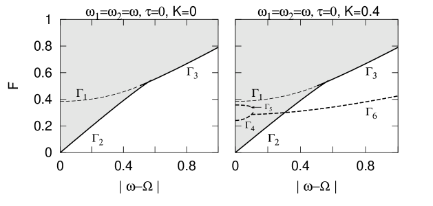
Figure 2: Bifurcation diagram of the in-phase solutions of identical oscillators with no delay. The shaded region represents the stability region of $Z_{1,2}=Re^{i(\Omega t+\alpha)}$.

In Fig. 2 all these critical curves are plotted for two different values of $K$. Notice that for $\tilde{\omega}=0$, the eigenvalues become $\{1-R^{2},1-3R^{2}\}$. So the branch of the fixed points ($\gamma$) falling above $R_{1,2}=1$ is stable for all $F$, and that below is unstable. This lower boundary of stability is given by $\Gamma_{2}$. The two unstable branches arising due to multiplicity of $\gamma$ merge on and disappear above $\Gamma_{1}$. At large values of $\tilde{\omega}$, the lower boundary of stability region is $\Gamma_{3}$. When $1/\sqrt{3}<\left|\tilde{\omega}\right|<1/2$, the curve $\gamma$ acquires stability in its multi-valued region leading to bistability of fixed points. The shaded region in Fig. 2 thus represents the stability region in which the system has at least one stable fixed point.

The stability analysis also produced an additional set of three curves $\Gamma_{4}$, $\Gamma_{5}$ and $\Gamma_{6}$ which, for $K=0$ merge with the curves $\Gamma_{1}$, $\Gamma_{2}$ and $\Gamma_{3}$ respectively, and do not exist for $K>0.5$. These indicate the intersections or mergers of other possible solutions of the system with the in-phase solutions studied above. A closed form for these solutions is not possible. But all such existing solutions can, in principle, be determined from the algebraic relations $\dot{Z}_{1.2}=0$ by setting $\omega_{1}=\omega_{2}=\omega$.

III.1 Amplitude response and frequency jumps

We now study the response of the system as a function of $F$. The response of the system in the region of stable synchronized solution is given by Eq. (12). In particular notice that since the basic oscillator has the limit cycle solution with a fixed amplitude of unity, the response is always linear for small amplitudes as a function of $F$. And at large amplitudes, the response is nonlinear: $R\propto F^{1/3}$. The in-phase oscillations will be locked to the external frequency with a phase difference $\alpha=0$ when $\tilde{\omega}=0$ (i.e. when they are driven resonantly), and with a phase difference $\alpha=\pi$ on the curve $F=\tilde{\omega}$.

Since the stable region for small $F$ is accessible only for $\left|\omega-\Omega\right|=0$, it is only when the system is driven with $\omega$ that a synchronization with the external frequency occurs for small $F$. Otherwise the system always goes to a two frequency state.

It is now left to determine the nature of the system in the region where the symmetric in-phase solution is unstable. Of particular interest is the average frequency of the system when compared to the frequency of the driving. In Fig. 3 the quantity $<\dot{\theta}>/\Omega$ is plotted as a function of $\left|\omega-\Omega\right|$ while keeping $\Omega=10$. The plot shows that this quantity has a finite jump across $\Gamma_{3}$ and no jump across $\Gamma_{2}$ which is consistent with the fact that on the critical curve $\Gamma_{3}$ there is a finite imaginary quantity of the eigenvalue, where as on $\Gamma_{2}$, the imaginary quantity is zero (and hence the frequency is equal to the external frequency). In fact the jump $(J)$ is directly related to the imaginary quantity on the critical curves across which the transition takes place:

$$J=\sqrt{(\omega-\Omega)^{2}-\frac{1}{4}}$$

Figure 3: Frequency transitions for different value of $F$ as $\left|\omega-\Omega\right|$ is increased.

Finally it should be remarked that for identical oscillators, region I (see Fig. 1) corresponding to incoherent states (for $F=0$) does not exist. Hence the above transition curve is the only relevant one.

III.2 Effect of finite dispersion

Finite dispersion facilitates the synchronization mechanism as we describe in this section using bifurcation diagrams. As seen in Fig. 1 regions $A$ and $B$ together make up the amplitude death region in the absence of an external force. The region is bounded by the curves $K=1$ and $K=\gamma(\Delta)=\frac{1}{2}(1+\Delta^{2}/4)$. The eigenvalues that determine the stability of this steady state are given by $\lambda=1-K\pm i\bar{\omega}\pm\sqrt{K^{2}-\Delta^{2}/4}$. The regions $A$ and $B$ are separated by the curve $K=\Delta/2$. Note that the system in the death state shows only one collective frequency $f=\bar{\omega}$, which occurs in region $B$. In region $A$, i.e, when $K<\Delta/2$, the oscillators spiral to the death state with independent frequencies: $f_{1,2}=\bar{\omega}\pm\sqrt{\Delta^{2}/4-K^{2}}$. In the presence of $F$, the external frequency interacts with $f_{1,2}$ and $f$ in the regions $A$ and $B$ respectively. Since the system offers damping to these modes, the system as a whole acts like a damped nonlinear oscillator with these characteristic frequencies. Thus the frequency of oscillation under forcing in both the regions is that of the external driver. The region of stability of this driven synchronization (i.e. the solution $Z_{1,2}=R_{1,2}{\mathrm{e}}^{i(\Omega t+\alpha_{1,2})}$) will have to be self consistently determined using the eigenvalue equation described in the previous section. Hence in the presence of $F$, the region of death now transforms into an oscillatory region in which both the oscillators synchronize with one another and also synchronize with the external frequency. The actual region of stability of the synchronized solution envelops the earlier death region. Before we present the stability region of this solution, we make some observations about the response of the individual oscillators. Without loss of generality, let us assume $\omega_{1}>\omega_{2}$. If $\Omega>\bar{\omega}$, then $R_{1}>R_{2}$. If $\Omega=\bar{\omega}$, then $R_{1}=R_{2}$. And if $\Omega<\bar{\omega}$, then $R_{1}<R_{2}$. At the resonant driving, the sum of the phases of the oscillators with respect to the external driver will be $0$. i.e. $\alpha_{1}+\alpha_{2}=0$.

We now briefly describe the solutions when the oscillators are driven resonantly, i.e. when $\Omega=\bar{\omega}$. At resonant driving, it is possible to arrive at a simpler set of algebraic equations to determine the amplitudes and the phase of this oscillatory state. Substituting $R_{1}=R_{2}=R$ and $\alpha_{2}=-\alpha_{1}$ in Eqs. (4-7), the following two relations can be written down that describe the amplitude and the phase of the system.

$$R={F\sin\alpha_{1}}/[\tilde{\omega}_{1}-K\sin(2\alpha_{1})],$$

where $\alpha_{1}$ is determined from the following functional relation:

$$g(\alpha_{1})=F^{2}\sin^{3}\alpha_{1}-(\tilde{\omega}_{1}-K\sin(2\alpha_{1}))^{2}[1-K+K\cos(2\alpha_{1})]\sin\alpha_{1}-(\tilde{\omega}_{1}-K\sin(2\alpha_{1}))^{3}\cos\alpha_{1}=0.$$

The response grows linearly with force. The dependence of $\alpha$ however is not apparent from the equation. Notice that the resonant point does not necessarily fall on the critical point of Hopf-bifurcation. The response of the oscillators and the phases are shown in Fig. 4 as a function of both $K$ and $F$. For small $F$, $R$ grows linearly, and for large $F$, it grows sub-linearly according to $R\propto F^{1/3}$. The scaling of the amplitude as a function of $F$ in a linear fashion is in accordance with the fact that inside the region of death state, the driven oscillator shows a linear response.

The coupled system shows an interesting response as a function of $K$. Increasing $K$ will sweep the stable synchronized region. For small $K$, the system shows incoherence, which is marked with dashed lines. The synchronized response loses stability at large values $K$ in a Hopf bifurcation. Close to this critical boundary, the phase of of the first oscillator as shown in the figure damps as $1/F$. However, the amplitude has a very nonlinear behavior as a function of $F$. It can be considered as linear only in the middle of the stability region.

Figure 4: Dependence of $R$ and $\alpha_{1}$ on $K$ and $F$. (a) and (b) are plotted for $F=1$, and (c) and (d) are plotted for $K=5$. The other parameters for all the plots are $\bar{\omega}=10$, $\Delta=18$, $\Omega=10$, and $\tau=0$.

Note, however, that since the region encompasses a Hopf bifurcation curve, $\gamma(\Delta)$, the response of each of the oscillators becomes nonlinear and proportional to $F^{1/3}$ on this curve. This characteristic nonlinear response at the Hopf bifurcation threshold has been invoked earlier to model the behavior of inner hair cells in human cochlea Camalet et al. (2000); Eguíluz et al. (2000). In the present context of two coupled oscillators, we have numerically verified this feature. The phase $\alpha_{1}$, which is a measure of the phase difference the first oscillator maintains with the driver, is nonzero, and is nearly constant for all weak forces, but damps with an approximate scaling of $F^{-0.4}$ for large values of $F$. The dotted curve drawn is only an indication of the power law. This behavior was not noted in literature before and may have some practical applications.

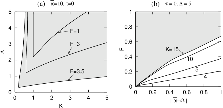
Figure 5: Stability regions (shaded) of the synchronized solutions $Z_{1,2}=R_{1,2}{\mathrm{e}}^{i(\Omega t+\alpha_{1,2})}$ when $\tau=0$ (a) for various $F$ when $\bar{\omega}=10$, (b) in $(F,\left|\tilde{\omega}\right|)$.

The coefficients of the eigenvalue equation (9) reveal that the stability is a function of the product term $\Omega\tau$. Thus the stability region in the absence of time delay is independent of $\Omega$ and only depends on $F$. We now present the stability regions of this synchronized state in the parametric space of $(K,\Delta)$ for different values of $F$ in Fig. 5(a). For weak forcing, the oscillators can be moved out of the synchronized regime by strongly coupling them. But as the forcing strength increases, much stronger or much weaker coupling is required to destabilize the synchronized state. At weaker couplings, it is the dispersion ($\Delta$) that is responsible for instability, and at stronger couplings, the system is more likely to get locked to its average frequency than to the external frequency. The relation between $F$ and $\left|\bar{\omega}-\Omega\right|$ is shown in Fig. 5(b). At larger values of $K$, a strong force is required to synchronize the system to the external frequency. When these solutions become unstable, there are two other possible solutions that are similar in character to the synchronized, and the incoherent states of the non-driven system. For any of the parameters corresponding to the bifurcation diagrams in Fig. 5(a), we note that the system’s average frequency is locked to the average frequency $\bar{\omega}$ of the oscillators for small value of $\Delta$. A numerical plot of the averaged frequency is shown in Fig. 6(a) which reveals that the transition from one coherent state to another is discontinuous. The nature of bifurcation at this transition is supercritical Hopf as can be seen from Fig. 6(b).

Figure 6: The time averaged quantities $<\dot{\theta}_{1,2}>$ and $<r_{1,2}>$ plotted in (a) and (b) respectively.

IV Nature of Synchronization in the presence of time delay

In this section we investigate effect of time delay on the forced synchronization of the coupled system. We again start our analysis by considering the instructive case of identical oscillators. We will study here the in-phase solutions under finite force. As in the previous section, under the assumption of the in-phase solutions, the study of Eqs. (1) and (2) becomes identical to studying a single oscillator with a delayed linear feedback and constant external forcing. Thus, it is sufficient to focus on the following equation:

$$\dot{Z}(t)=(1-K+i\omega-\left|Z(t)\right|^{2})Z(t)+KZ(t-\tau)+F{\mathrm{e}}^{i\Omega t}$$ (16)

or under the transformation $Y(t)=Z(t){\mathrm{e}}^{-i\Omega t}$,

$$\dot{Y}(t)=(1-K+i\tilde{\omega}-\left|Y(t)\right|^{2})Y(t)+K{\mathrm{e}}^{-i\Omega\tau}Y(t-\tau)+F,$$ (17)

where $\tilde{\omega}=\omega-\Omega$. Substituting $Y=R{\mathrm{e}}^{i\alpha}$ in Eq. (17) and separating the real and imaginary parts one arrives at the following two equations:

$$(1-K-R^{2})R+KR\cos(\Omega\tau)+F\cos\alpha=0,$$

$$\tilde{\omega}R-KR\sin(\Omega\tau)-F\sin\alpha=0,$$

which can be algebraically simplified to arrive at the following expressions for determining $R$ and $\alpha$:

$$R^{6}+a_{2}R^{4}+a_{1}R^{2}-F^{2}=0,$$ (18)

$$\alpha=\cases{\sin^{-1}\frac{bR}{F}&~{}~{}if~{}~{} $c<R^{2}$,\cr\pi-\sin^{-1}\frac{bR}{F}&~{}~{}if~{}~{} $c\geq R^{2}$.}$$ (19)

where $b=\tilde{\omega}-K\sin(\Omega\tau)$, $a_{1}=b^{2}+c^{2}$. $a_{2}=-2c$, and $c=1-K+K\cos(\Omega\tau)$. Eq. (18) produces a curve $R=\gamma(\tilde{\omega},K,\Omega\tau,F)$ which can be multiple-valued. The number of real roots for ${R}^{2}$ now ranges from one to three. The stability of these solutions that can be determined from $M$ are governed by the following eigenvalue equations,

$$\lambda=1-K-2{R}^{2}+s_{k}K{\mathrm{e}}^{-\lambda\tau}+s\sqrt{{R}^{4}-\tilde{\omega}^{2}},\\$$ (20)

where $s_{k}=\pm 1$ and $s=\pm 1$. These two signs must be taken in all the permutations. Thus we have four transcendental equations. It is possible to treat all these equations together. Just as we did in the no-delay case, we consider here also two cases (i) ${R}^{2}>\left|\tilde{\omega}\right|$ and (ii) ${R}^{2}\leq\left|\tilde{\omega}\right|$. In the first case, in order to arrive at the critical curves across which transitions of eigenvalues take place, we set $\lambda=i\beta$. This gives the following two equations:

$$1-K-2{R^{*}}^{2}+s\sqrt{{R^{*}}^{4}-\tilde{\omega}^{2}}=-s_{k}K\cos(\beta\tau),$$ (21)

$$\beta=-s_{k}K\sin(\beta\tau).$$ (22)

Note that $\beta=0$ is a solution of the Eq. (22) for any value of $K$ and $\tau$. This branch corresponds to the critical curves that existed for the case of $\tau=0$ when both $s$ and $s_{k}$ are considered independently. For a second branch of solution for Eq. (22) to exist, the necessary condition is $K\tau>1$. Again from Eq. (22), it can further be concluded that the critical values of $K\tau$ beyond which the second branch exists are determined from the zeros of the function $g=\cos(\sqrt{K^{2}\tau^{2}-1})+1/(s_{K}K\tau)$. A numerical analysis of the equation $g=0$ gives the critical values: $K\tau=4.6034$, if $s_{K}=1$, and $K\tau=1$, if $s_{k}=-1$. A set of critical curves for the second and higher branches are obtained by explicitly considering $s=\pm 1$ of the newly generated branches. Also note that the response now is a function of $\tau$. Hence the stability can be affected by the $\beta=0$ branch itself. An equation for $R^{2}$ can be written down by eliminating $\beta$ as follows:

$$\beta=\left\{K^{2}-\left[1-K-{R^{*}}^{2}+s\left\{{R^{*}}^{4}-\tilde{\omega}^{2}\right\}^{1/2}\right]^{2}\right\}^{1/2},$$ (23)

$${R^{*}}^{2}=\frac{1}{2}\left(1-K+s_{k}K\cos(\beta\tau)+s\sqrt{{R^{*}}^{4}-\tilde{\omega}^{2}}\right).$$ (24)

The critical curves in $(F,\tilde{\omega})$ plane cannot in general be written down in a closed form as we did for the case of $\tau=0$. The conditions that exist on $K$, and $\tilde{\omega}$ must now be determined using the two transcendental equations above. These equations can be used along with Eq. (18) to numerically plot the critical curves in $(F,\tilde{\omega})$ plane by setting $R^{2}={R^{*}}^{2}$. We can easily identify that the curves that are counterparts of $\Gamma_{1}$ and $\Gamma_{2}$ of the no-delay case are generated here by setting $s_{k}=1$. The critical curves corresponding to $\beta=0$ can, however, be determined in closed form. Following a similar analysis as outlined in the Appendix, these curves are obtained as

$$\Gamma_{1}^{\prime}=\left\{F=f(\rho_{+})\big{|}\rho_{+}=\frac{2}{3}+\frac{1}{3}\sqrt{1-3\tilde{\omega}^{2}}\right\},\omega^{2}\in[0,\frac{1}{3}],$$ (25)

$$\Gamma_{2}^{\prime}=\left\{F=f(\rho_{-})\big{|}\rho_{+}=\frac{2}{3}-\frac{1}{3}\sqrt{1-3\tilde{\omega}^{2}}\right\},\omega^{2}\in[0,\frac{1}{3}],$$ (26)

where $f(\rho)=\{\rho^{3}+a_{2}\rho^{2}+a_{1}\rho\}^{1/2}$. These are the only critical curves that exist under this case as long as $K\tau<1$. If this condition is violated pairs of sets of such critical curves exist.

In the second case, i.e. when ${R}^{2}\leq\left|\tilde{\omega}\right|$, on the critical curves, we again set $\lambda=i\beta$ to arrive at the following set of equations:

$$1-K-2{R^{*}}^{2}=-s_{k}K\cos(\beta\tau),$$ (27)

$$\beta+s_{k}K\sin(\beta\tau)=s\sqrt{{R^{*}}^{4}-\tilde{\omega}^{2}}.$$ (28)

Note that since the eigenvalues occur in complex conjugate pairs, the second of the above two equations yields the same set of curves for both $s=\pm 1$. So there will be two classes of curves corresponding to $s_{k}=\pm 1$. The above two equations can further be simplified to yield

$$\beta=\beta_{\pm}=\sqrt{\tilde{\omega}^{2}-{R^{*}}^{4}}\pm\sqrt{K^{2}-(1-K-2{R^{*}}^{2})},$$ (29)

$${R^{*}}^{2}=\frac{1}{2}\left(1-K+s_{k}K\cos(\beta\tau)\right).$$ (30)

The second set of critical curves, $\Gamma_{3}^{\prime}$, in $(\tilde{\omega},F)$ plane are obtained using the above two equations along with Eq. (12) by setting $R^{2}={R^{*}}^{2}$. We can again identify that the counterpart of the curve $\Gamma_{3}$ of the no-delay case is obtained here by setting $s_{k}=1$. As $\tau$ is increased, the parameter region falling below the curve $\Gamma_{3}$ becomes more and more susceptible for synchronization, and in fact for a range of value of $\tau$ the curve makes intersections with $F=0$ line as shown in Fig. 7. The region marked I is the region of stability of the synchronized solution. At the region of intersection of the three curves, there is also a possibility of more than one synchronized solution coexisting.

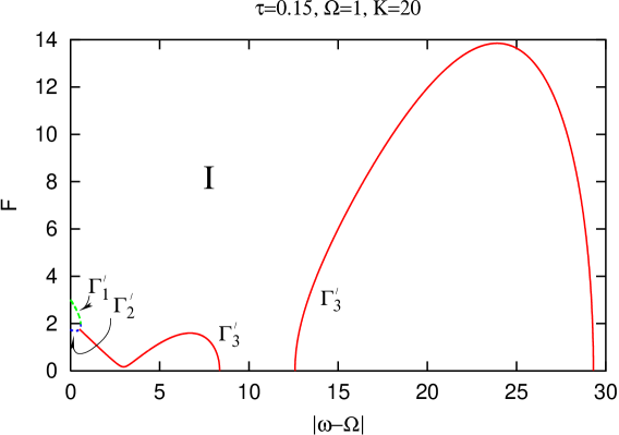
Figure 7: The critical curves $\Gamma_{1}^{\prime}$, $\Gamma_{2}^{\prime}$, and $\Gamma_{3}^{\prime}$, in the presence of $\tau$ at $K=20$, $\Omega=1$, and $\tau=0.15$. Region I represents the synchronized region.

At higher values of time delay, a stronger force is required to make the oscillators synchronize with the external driver. The other set of curves that are generated using the second sign $s_{k}=-1$ represent intersections of the response of the system with other unstable solutions the system possesses. We do not discuss them here. This figure depicts one of the important results of our present paper. In the presence of appropriate time delay the region of forced synchronization can be extended to continuously connect with $F=0$ axis. This raises the interesting possibility of achieving synchronization far from resonant driving with a minimal (nearly infinitesimal) force.

The role of time delay can be more clearly appreciated by determining the required critical curves in the plane of $(\tau,K)$. By following the usual analysis of such characteristic equations and properly choosing the correct signs for the cosine function above, the critical curves in the plane of $(K,\tau)$ can easily be derived. When ${R^{*}}^{2}>\left|\tilde{\omega}\right|$, the equations for $R$ and $\beta$ at criticality, Eqs. (21) and (22) can be used to derive an equation for $\tau$ in terms of $K$:

$$\tau_{\pm}=\frac{n\pi-\cos^{-1}\left(\frac{-A_{\pm}}{K}\right)}{\sqrt{K^{2}-A_{\pm}^{2}}},$$ (31)

where $A_{\pm}=1-K-2{R^{*}}^{2}\pm\sqrt{{R^{*}}^{4}-\tilde{\omega}^{2}}$. On both of the above two curves, $\tau_{\pm}$, the nature of the transition of the eigenvalues is given by:

$$\frac{d}{d\tau}Re(\lambda)\Big{|}_{Re(\lambda)=0}>0.$$ (32)

Thus these two curves in the $(\tau,K)$ space represent critical curves across which a pair of eigenvalues makes transition to acquire positive real parts.

In the second case, i.e. when ${R^{*}}^{2}\leq\left|\tilde{\omega}\right|$, the valid equations are Eqs.  (27) and (28). By again following the standard methods to derive the critical curves, we arrive at the following set of two marginal stability curves:

$$\tau_{1}=\frac{n\pi-\cos^{-1}\left(\frac{1-K-2{R^{*}}^{2}}{-K}\right)}{\sqrt{\tilde{\omega}^{2}-{R^{*}}^{4}}+\sqrt{K^{2}-(1-K-2{R^{*}}^{2})^{2}}},$$ (33)

$$\tau_{2}=\frac{n\pi+\cos^{-1}\left(\frac{1-K-2{R^{*}}^{2}}{-K}\right)}{\sqrt{\tilde{\omega}^{2}-{R^{*}}^{4}}-\sqrt{K^{2}-(1-K-2{R^{*}}^{2})^{2}}}.$$ (34)

The nature of transition of the eigenvalues across these critical curves is given by:

$$\frac{d}{d\tau}Re(\lambda)\Big{|}_{Re(\lambda)=0}\cases{>0~{}~{}{\mathrm{o}n}~{}~{}\tau_{1},\cr<0~{}~{}{\mathrm{o}n}~{}~{}\tau_{2}.}$$ (35)

The curves $\tau_{\pm}$ and $\tau_{1,2}$ completely describe the stability transition curves in $(\tau,K)$ space for a given set of $F$ and $\omega$. The ordering of these curves depending on $F$ and $\omega$ will eventually determine the curves that enclose the stable regions.

IV.1 Amplitude response and frequency jumps

We now examine the response of the system. Notice from Eq. (18) that the oscillators respond linearly with $F$ for small amplitudes (i.e. when the $F^{2}$ term is balanced by the $a_{1}R^{2}$ term). For larger amplitudes the response becomes nonlinear as the balance is provided by other terms. However the response can be highly nonlinear even for small amplitudes on certain contours of the parametric space where $a_{2}=0$, and $a_{1}=0$. Under these conditions the following two equations are obtained (provided that $\Omega\tau\neq 2n\pi$):

$$\cos(\Omega\tau)=(1-K)/K,$$

and

$$\sin(\Omega\tau)=(\omega-\Omega)/K.$$

Using the above two equations we can derive the conditions relating $K$ and $\Omega\tau$ for a given $\tilde{\omega}$ such that the response of the system for small amplitudes has a nonlinear character ($R\propto F^{1/3}$):

$$K = (1+\tilde{\omega}^{2})/2,$$ (36)

$$\Omega\tau = 2n\pi+\cos^{-1}\left(\frac{1-\tilde{\omega}^{2}}{1+\tilde{\omega}^{2}}\right).$$ (37)

In the $(F,\tilde{\omega})$ plane, the corresponding contours can be derived from Eq. (18) by making use of the above two relations. We will discuss this phenomenon in more detail later. At the boundary of stability region, the oscillators make a transition in their average frequency from their intrinsic average frequency to that of the driver. This discontinuity is a function of $\tau$ and is numerically found to be quadratic in its dependence on $\tau$ as shown in Fig. 8.

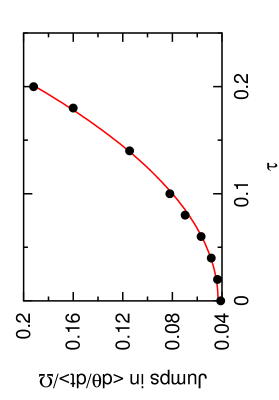
Figure 8: Jumps of the average frequency across the critical boundary separating synchronous and non-synchronous regions. $K=0.4$, $F=0.6$, $\Omega=10$. Bullets are numerically found values. The curve is a best fit with $3.685\tau^{2}+0.043$.

IV.2 Effect of finite dispersion

We now study the effect of finite time delay and the external force on non-identical oscillators. Our primary objective is to examine the stability properties of the synchronized state $Z_{1,2}=R_{1,2}{\mathrm{e}}^{i(\Omega+\alpha_{1,2})}$ which is also synchronized with the external frequency. We use Eqs. (4-7) to determine the responses $R_{1,2}$, and $\alpha_{1,2}$ and then find the eigenvalue spectrum to determine their stability. The response due to time delay shows considerable deviation from the no-delay case. Under certain conditions, both the oscillators could have identical amplitudes. Similar to our studies in the previous section, we assume that $R_{1}=R_{2}=R$ and $\alpha_{1}+\alpha_{2}=0$. This ansatz leads to the condition that $\Omega\tau=\pi$. Substituting these relations in Eqs. (4-7), we arrive at the following two simplified equations for the responses:

$$\cos\alpha_{1} = -\frac{R}{F}\left(1-K-R^{2}-K\cos(2\alpha_{1})\right),$$

$$\sin\alpha_{1} = \frac{R}{F}\left(\tilde{\omega}_{1}+K\sin(2\alpha)\right),$$

which can further be simplified to arrive at an equation for $R$ as a function of $\alpha_{1}$ as

$$R={F\sin\alpha_{1}}/[\tilde{\omega}_{1}+K\sin(2\alpha_{1})],$$ (38)

and a functional relation to determine $\alpha_{1}$ as

$$h(\alpha_{1})=F^{2}\sin^{3}\alpha_{1}-(\tilde{\omega}_{1}+K\sin(2\alpha_{1}))^{2}[1-K-K\cos(2\alpha_{1})]\sin\alpha_{1}-(\tilde{\omega}_{1}+K\sin(2\alpha_{1}))^{3}\cos\alpha_{1}=0.$$

The above expression for $\cos\alpha_{1}$ again indicates that for this special case the response of the oscillators is nonlinear according to $R\propto F^{1/3}$ at large values of $F$.

However, the amplitudes of the oscillators are in general not identical. The response of the oscillators in the synchronized state is unique only when $0\leq\Omega\tau<2\pi$. In Fig. 9 the amplitudes and phases are shown as a function of $\tau$. For a given $\tau$, stronger coupling among oscillators decreases the amplitudes. At $\Omega\tau=\pi$, the oscillators are locked with the external driver with a maximum phase difference.

Figure 9: Amplitudes and phases of the oscillators as a function of $\tau$.

For a given set of parameters the external forcing will widen the region of stability of the synchronized solution. In Fig. 10(a) the response of one of the oscillators is plotted for different values of $F$. The boundary of the stability regions of the death state in the absence of external driving falls inside the stability region of the synchronized state. In Figs. 10(b), (c), and (d), the stability region of the synchronized state is shown in $(K,\Delta)$ space for three different values of the driving frequency $\Omega$ and a fixed set of $F=1.0$, $\tau=0.05$, and $\bar{\omega}=10$. In each of these figures, the dashed curve indicates the marginal stability curve for $F=0$. As is evident the stability region of the tuned state is sensitive to $\Omega$ and appears to increase in area for slow driving. The difference between the effects of force (as seen from Fig. 5) and that of time delay is evident here in the bifurcation diagram. Time delay breaks up the degenerate bifurcation point where as just the presence of force alone would not remove the degeneracy.

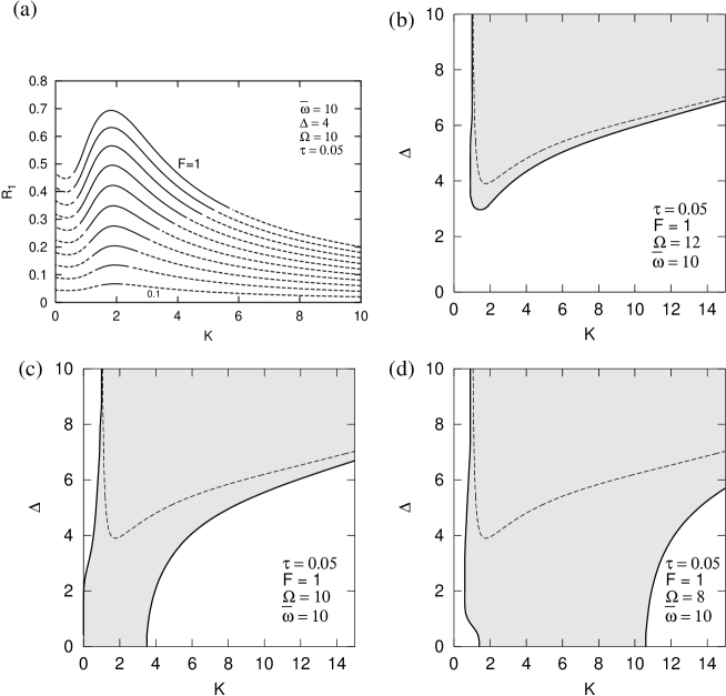
Figure 10: (a) Response of the first oscillator for various $F$ as a function of $K$. Stability regions (shaded) of the tuned state in $(K,\Delta)$ space for (b) $\Omega=12$, (c) $\Omega=10$, (d) $\Omega=8$, while keeping the other parameters at $F=1$, $\tau=0.05$, and $\bar{\omega}=10$.

Finally we examine the average frequencies as a function of the frequency dispersion. In the absence of time delay, as we noted in the previous section, there is a transition of the average frequencies to the external frequency as $\Delta$ is increased. However, in the presence of time delay, the intrinsic frequencies are affected by $\tau$ differently, and thus there could be connected regions of $\tau$ where the oscillators can be found in two different locked states as shown in Fig. 11. Here the first oscillator with small frequency (left curve in the frequency plot) is more susceptible to the external driving and gets locked to it at a smaller value of $\Delta$ while the second one is still locked to the branch of the average intrinsic frequency. The corresponding amplitudes are shown in Fig. 11(b). This feature is absent for $\tau=0$ and may be found in multiple connected regions of $\tau$.

Figure 11: Average frequencies and the average amplitudes as a function of $\Delta$. The first of the two oscillators has smaller frequency. In (a) the left vertical curve corresponds to the first oscillator. $F=1$, $\tau=0.2$, $\bar{\omega}=10$, $\Omega=2$, and $K=1.5$.

IV.3 Tuning property of time delay

Having now found the region of stability of the tuned solutions, we must then examine the response of the oscillators in this region and find where the maximum or resonant response occurs and with what functional relation this response scales with the driving force, $F$. The Hopf bifurcation curves of the non-driven system in the presence of finite $\tau$ have a special significance in that on them the response is nonlinear even for small $F$. This fact was noted earlier in the literature and was used to model the nonlinear compression of sound frequencies by the inner hair cells of the cochlea Camalet et al. (2000); Eguíluz et al. (2000). In the presence of $\tau$ the frequency on such critical curves has a dependence on $\tau$. This makes it possible to choose a proper time delay such that a nonlinear response at a given external frequency is achieved.

Figure 12: (a) Two of the intrinsic frequencies existing in the undriven system. The solid portions of the curves represent damped regions, i.e. the real part of the corresponding eigenvalue has negative sign. The bullets indicate the values of $K$ at which the damping of that particular mode is zero, (b) The tuned frequency as a function of $\tau$. (c) Resonances on the tuned frequency curve. (d) The amplitude response of one of the oscillators on and around the tuned frequency curve. The curve $\gamma_{1}$ is a straight line with slope unity, and $\gamma_{2}$ is that with 3.

We explore this interesting feature further by examining the eigenvalue spectrum of the death state in the absence of external force. The eigenvalue equation that determines the stability of the origin is

$$\lambda=1-K\pm\sqrt{K^{2}{\mathrm{e}}^{-2\lambda\tau}-\Delta^{2}/4}\pm\bar{\omega}$$ (39)

which can be derived from Eq. 9 by inserting $R_{1,2}=0$. We are now interested in the imaginary parts of the eigenvalues. The real parts only reveal the damping of that particular frequency mode when the driving is turned on. A detailed study of the marginal stability was earlier carried out in literature. Here we examine the imaginary parts of the eigenvalue spectrum (i.e. the intrinsic frequencies of the system) as a function of $K$. As can be verified from the full spectrum, the lower frequencies are least damped and the higher frequencies are heavily damped. So we focus our attention on the first two frequencies of the system. Since the eigenvalues occur in complex conjugate pairs, it is sufficient to plot the positive frequencies. In Fig. 12(a), the intrinsic frequencies of the eigenvalue spectrum are plotted while showing the nature of the damping existing for each branch. The system responds linearly to the external driving in the region of damping. The two frequencies plotted have critical points on them marked $a$, $b$ and $c$. A nonlinear growth of the amplitude of the oscillators occurs at all the points $a$, $b$, and $c$ as a function of the driving force at any given value of $\Omega$. The higher frequency branch has only one critical point $a$ at which the damping is zero. To the left of the point, the frequency is a growing mode and to the right, the frequency is a damped mode. Also note that the region left to point $a$ indicates a drift region. The lower branch has two critical points on it: $b$ and $c$ both representing zero growth of the mode. The region left to the point $b$ and that to the right of $c$ are growing modes. The critical points $a$ and $b$ are not sensitive to variations in $\tau$ and thus their frequency span is too limited. However the point $c$ is sensitive to $\tau$ and in fact spans a range of $\Omega$ values as $\tau$ is increased. Thus this point is of interest to us. At higher values of $\Delta$, a large frequency range can be spanned with a short variation in $\tau$. In Fig. 12(b) the contour of $c$ is plotted in $(\Omega,\tau)$ space. At this frequency the system responds nonlinearly and can be termed as the tuned frequency. In Fig. 12(c) the frequency response of the system is shown as one traverses along the tuned frequency curve shown in Fig. 12(b) for $\Delta=10$.

Now we show the response of the oscillators at the tuned frequencies. The system responds nonlinearly with the amplitude proportional to $F^{1/3}$. In Fig. 12(d) the amplitude of one of the oscillators is plotted in log-scale for a choice of the parameters lying on the tuned frequency curve shown in Fig. 12(b): $K(=K^{*})=16.861411237$, $\tau=0.06$, $\Omega=(\Omega^{*})=4.968163$, $\bar{\omega}=10$, $\Delta=6$. The responses around the curve are linear, but on the critical curve the response is nonlinear and is proportional to $F^{1/3}$.

V Synchronization of a large number of coupled oscillators

We now briefly consider the question of the possibility of synchronizing a large group of globally coupled oscillators that have a distribution of frequencies, $g(\omega)$, and are driven by an external periodic force:

$$\dot{Z}_{j}(t)=(1+i\omega_{j}-\left|Z_{j}(t)\right|^{2})Z_{j}(t)+\frac{K}{N}\sum\limits_{k=1}^{N}[Z_{k}(t-\tau)-Z_{j}(t)]+F{\mathrm{e}}^{i\Omega t},$$ (40)

The contribution of the self coupling term that would emanate from the summation above would be ignorable as the size of the system becomes large. A full bifurcation picture of these equations is relegated to a future study. Here we present the main features exhibited by this system which are common to the case of two oscillators discussed so far. $g(\omega)$ is assumed to be in the form of uniform density distribution, i.e. $g(\omega)=1/2\gamma$ for $\omega\in[-\gamma,\gamma]$, and $0$ otherwise. The frequencies are chosen with equal spacing. Since time delay removes the symmetry enjoyed by the system, a constant positive value $\bar{\omega}$ is added to the frequency distribution to make all the frequencies positive. A convenient macroscopic parameter to characterize the collective properties of a large population of oscillators is the order parameter defined by

$$S=R(t){\mathrm{e}}^{i\Phi(t)}=\frac{1}{N}\sum\limits_{j=1}^{N}Z_{j}(t).$$ (41)

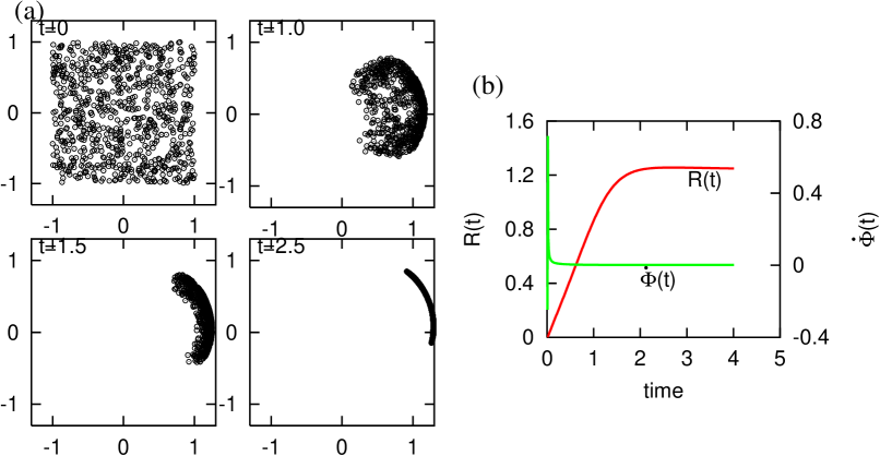
Figure 13: (a)$(X,Y)$ snapshots of time evolution of $800$ coupled oscillators under external force. (b) The evolution of the amplitude and the derivative of the phase of the order parameter in the moving frame. $\gamma=0.6$, $K=0.8$, $F=1$, $\tau=0.18$, $\Omega=1.0$, and $\bar{\omega}=1.2$.

In Fig. 13(a) the time evolution of $N=800$ oscillators are plotted in $(X,Y)$ plane in the frame moving with the external frequency for $F=1$, $\tau=0.18$, $\bar{\omega}=1.2$, and $\Omega=1.0$. A stationary asymptotic state in the fourth panel indicates a complete synchronization of all the oscillators in the population to the driving frequency. Since the forcing is strong, the synchronization time is short, and the coupling strength is overcome by $F$. In Fig. 13(b) magnitude ($R$) and the frequency ($\dot{\Phi}$ of the order parameter are plotted in the moving frame. This confirms the synchrony.

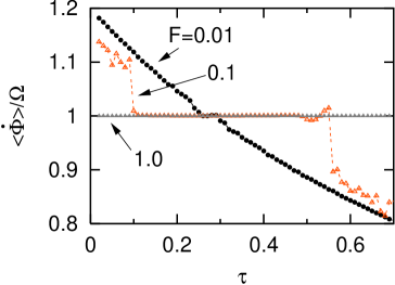
Figure 14: Synchronization regions for different $F$ as a function of $\tau$. $N=100$, $\gamma=0.6$, $K=0.8$, $\Omega=1.0$, and $\bar{\omega}=1.2$.

One of our important results in the earlier sections is the possibility of synchronization for infinitesimal forces in the presence of time delay. For this we carry out simulations on $N=100$ for finite time delay, and finite frequency spread for various values of driving force. The results are presented in Fig. 14 as a plot of $<\dot{\Phi}>/\Omega$ vs. $\tau$. For a strong force ($F=1$) the horizontal line indicates synchronization. The synchronization occurred here even for $\tau=0$ and extends to a very large value of $\tau$. As we decrease the force, synchronization at $\tau=0$ is lost, but is attained for a range of $\tau$ values. Even for $F=0.01$, this particular choice of $\gamma$ shows a range of $\tau$ values where synchronization is found. This confirms our earlier results on two coupled oscillators. Further work on the bifurcation structure of the large number of oscillators will be reported elsewhere.

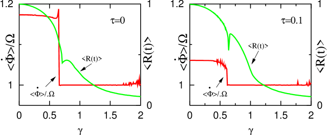
Figure 15: Frequency jumps shown as a function of $\gamma$ for (a) $\tau=0$, and (b) $\tau=0.1$. The other parameters are $N=100$, $K=0.8$, $F=0.1$, $\Omega=1$, and $\bar{\omega}=1.2$.

Finally we look at the frequency transitions from synchronization between the oscillators to that to the driving frequency. In Fig. 15(a) and (b) the average values of the amplitude of the order parameter $<R(t)>$, and the ratio of the average frequency to the driving frequency, $<\dot{\Phi}>/\Omega$ are plotted as a function of the frequency width $\gamma$ for $\tau=0$, and $\tau=0.1$. At lower values of $\gamma$, as is also evident even for two coupled oscillators, the oscillators are not synchronized to the driver, but make a transition to the synchronized state at a critical value. At large values of $\gamma$ synchronization loses its stability. The frequency of the collective state at lower $\gamma$ is suppressed by time delay.

VI Conclusions

We have carried out a detailed theoretical analysis of the driven periodic response of a system of two time delay coupled limit cycle oscillators that are subjected to identical external forces. In particular, we have examined the stability properties of periodic phase locked oscillations of the system that are synchronized with the external driving frequency. Bifurcation diagrams in the parameter space of the coupling strength and frequency spread of the two oscillators have been presented and their variation with time delay has been discussed. We have also obtained the characteristics of the response function in various limits and highlighted their sensitivity to time delay. We have further confirmed that some of the important results of the two oscillator system also emerge in simulations carried out on a large number of globally coupled limit cycle oscillators.

For the sake of completeness and to gain an overall perspective of our results we have also showed the connection of our work to earlier investigations of non-driven coupled oscillators, with Reddy et al. (2000b) or without Aronson et al. (1990) time delay, and to driven oscillators without time delay Guckenheimer and Holmes (1983). The parametric region corresponding to the amplitude death of two coupled non-driven oscillators has been the primary area of our interest. This is the region that sustains a periodic oscillation when the system is driven externally. For our time delayed system the extent of this region and the nature of the driven response within it are all sensitive functions of the driving frequency, driving amplitude and the time delay parameter. This is evident from the detailed results presented in the various previous sections. In general, the size of the stability region of the forced response is larger than the size of the original death region of the non-driven system. However the bounding curves of the original region play a special role in that the small amplitude response on them is highly nonlinear.

Two important results of our work are worth highlighting in view of their potential applications. First, by an appropriate choice of time delay, it is possible to mitigate the disadvantages of far from resonance driving and to achieve synchronization with a minimal of force. Second, for a fixed driving frequency, the driven response of the system can be tuned to any desired frequency with a suitable choice of the delay parameter. This property relies on the nonlinear response of the system on the Hopf bifurcation boundaries. Since the location of these boundaries (in the frequency space) is a sensitive function of time delay it provides for this possibility of using the time delay parameter as a control knob for frequency tuning. It would be interesting to look for evidences of these effects operating in natural biological and chemical systems or to implement them in appropriately designed electronic receiver systems.

Finally we would like to remark that in our analysis we have not examined the driven response in the region of phase drift solutions. Such a study is presently in progress as is the extension to a larger system of coupled oscillators where regions of chaotic solutions could be explored. Future work should also focus on large number of locally coupled oscillators.

*

Appendix A Derivation of Curves $\Gamma_{1}$ to $\Gamma_{6}$

In order to obtain the bifurcation diagram in $(F,\tilde{\omega})$ plane, we must find the critical curves of the above equations by setting Re$(\lambda)=0$. For the sake of convenience consider two cases: (i) ${R}^{2}>\left|\tilde{\omega}\right|$, and (ii) ${R}^{2}\leq\left|\tilde{\omega}\right|$. In either of these two cases the real part of the eigenvalues of Eq. (14) are always less by a positive value $2K$ than those of the Eq. (15). Thus, at the critical set of parameters where the first two equations have their real parts zero, the real parts of the other two equations are negative. Hence, it is obvious that the boundaries of the steady state are completely determined by the eigenvalues of Eq. (14) alone. In fact these two equations determine the stability of the curve $\gamma$. The other two equations provide critical curves that represent transitions of the eigenvalues. We find that the other solutions the system admits will merge with the in-phase solutions at these critical lines. First we derive the critical curves under both the cases mentioned above for Eq. (14). Then we treat the other two eigenvalue equations.

Considering Eq. (14) with $+$ sign under case (i), ${\mathrm{R}e}(\lambda)=1-2{R}^{2}+\sqrt{{R}^{4}-\tilde{\omega}^{2}}$, and ${\mathrm{I}m}(\lambda)=0$. The criticality occurs at ${\mathrm{R}e}(\lambda)=0$ (and thus $1-2{R^{*}}^{2}<0$), which results in $R^{2}={R^{*}}^{2}_{\pm}=2/3\pm\sqrt{1/9-\tilde{\omega}^{2}/3}$. Now by making use of Eq. (12), and the condition $1-2{R^{*}_{-}}^{2}<0$, the following critical curve ($\Gamma_{1}$) can easily be written down:

$$\Gamma_{1}:~{}~{}~{}~{}F=\left\{\frac{2}{27}\left[(1+9\tilde{\omega}^{2})+(1-3\tilde{\omega}^{2})^{3/2}\right]\right\}^{1/2},~{}~{}~{}\tilde{\omega}^{2}\in[\frac{1}{4},\frac{1}{3}].$$ (42)

Similarly, making use of Eq. (12), and the condition $1-2{R^{*}_{+}}^{2}<0$, the following critical curve ($\Gamma_{2}$) can be written down:

$$\Gamma_{2}:~{}~{}~{}~{}F=\left\{\frac{2}{27}\left[(1+9\tilde{\omega}^{2})-(1-3\tilde{\omega}^{2})^{3/2}\right]\right\}^{1/2},~{}~{}~{}\tilde{\omega}^{2}\in[0,\frac{1}{3}].$$ (43)

Under the case (i) again, Eq. (14) with $-$ sign yields ${\mathrm{R}e}(\lambda)=1-2{R}^{2}-\sqrt{{R}^{4}-\tilde{\omega}^{2}}$, and ${\mathrm{I}m}(\lambda)=0$. The criticality occurs at ${\mathrm{R}e}(\lambda)=0$ (and thus $1-2{R^{*}}^{2}>0$), which again results in $R^{2}={R^{*}}^{2}_{\pm}=2/3\pm\sqrt{1/9-\tilde{\omega}^{2}/3}$. Note that $R^{2}={R^{*}_{+}}^{2}$ fails to obey the condition $1-2{R}^{2}>0$. Hence $R^{2}={R^{*}_{+}}^{2}$ does not result in any critical curves. But $R^{2}={R^{*}_{-}}^{2}$ results in the following critical curve:

$$\Gamma_{1}:~{}~{}~{}~{}F=\left\{\frac{2}{27}\left[(1+9\tilde{\omega}^{2})+(1-3\tilde{\omega}^{2})^{3/2}\right]\right\}^{1/2},~{}~{}~{}\tilde{\omega}^{2}\in[0,\frac{1}{4}].$$ (44)

Under case (ii) Eq. (14) with both signs can be considered together: ${\mathrm{R}e}(\lambda)=1-2R^{2}$, and ${\mathrm{I}m}(\lambda)=\pm\sqrt{\tilde{\omega}^{2}-R^{4}}$. The criticality occurs at $R^{2}={R^{*}}^{2}=1/2$ with the condition that $R^{2}<\left|\tilde{\omega}\right|$. This, when substituted in Eq. (12), results in the following critical curve:

$$\Gamma_{3}:~{}~{}~{}~{}F=\left\{(\tilde{\omega}^{2}+1/4)/2\right\}^{1/2},~{}~{}~{}\tilde{\omega}^{2}\in[\frac{1}{4},\infty).$$ (45)

Since the imaginary part of the eigenvalue spectrum is nonzero, the nature of the bifurcation across this critical curve is determined by

$$\frac{d}{dF}{\mathrm{R}e}\lambda\Big{|}_{{\mathrm{R}e}\lambda=0}=\frac{-4F}{\tilde{\omega}^{2}-\frac{1}{4}}\cases{>0&~{}~{}if~{}~{} $\tilde{\omega}^{2}<\frac{1}{4}$,\cr<0&~{}~{}if~{}~{} $\tilde{\omega}^{2}>\frac{1}{4}$,}$$ (46)

which indicates that the bifurcation is of the supercritical Hopf kind.

We now consider Eq. (15) with $+$ sign under case (i): ${\mathrm{R}e}(\lambda)=1-2K-2R^{2}+\sqrt{R^{4}-\tilde{\omega}^{2}}$, and ${\mathrm{I}m}(\lambda)=0$. Let us define $f(\rho)=\{\rho^{3}-2\rho^{2}+(1+\tilde{\omega}^{2})\rho\}^{1/2}$, and $a=2K-1$. Following exactly the same method as described above, the critical curves can be derived as follows for $K<\frac{1}{2}$:

$$\Gamma_{4}:F=\{f(\rho_{-})~{}\Big{|}~{}\rho_{-}=\frac{-2a}{3}-\sqrt{\frac{a^{2}}{9}-\frac{\tilde{\omega}^{2}}{3}}\},~{}~{}\tilde{\omega}^{2}\in[a^{2}/4,a^{2}/3],$$ (47)

$$\Gamma_{5}:F=\{f(\rho_{+})~{}\Big{|}~{}\rho_{+}=\frac{-2a}{3}+\sqrt{\frac{a^{2}}{9}-\frac{\tilde{\omega}^{2}}{3}}\},~{}~{}\tilde{\omega}^{2}\in[0,a^{2}/3].$$ (48)

And using the Eq. (14) with $-$ sign, the corresponding curve turns out to be:

$$\Gamma_{4}:F=\{f(\rho_{-})~{}\Big{|}~{}\rho_{-}=\frac{-2a}{3}-\sqrt{\frac{a^{2}}{9}-\frac{\tilde{\omega}^{2}}{3}}\},~{}~{}\tilde{\omega}^{2}\in[0,a^{2}/4].$$ (49)

Still under case (i), the nature of the curves under $K>\frac{1}{2}$ differ from the above. The curves are derived using the same method as above. Eq. (14) with $-$ sign results in

$$\Gamma_{4}:F=\{f(\rho_{-})~{}\Big{|}~{}\rho_{-}=\frac{-2a}{3}-\sqrt{\frac{a^{2}}{9}-\frac{\tilde{\omega}^{2}}{3}}\},~{}~{}\tilde{\omega}^{2}\in[0,a^{2}/3].$$ (50)

$$\Gamma_{5}:F=\{f(\rho_{+})~{}\Big{|}~{}\rho_{+}=\frac{-2a}{3}+\sqrt{\frac{a^{2}}{9}-\frac{\tilde{\omega}^{2}}{3}}\},~{}~{}\tilde{\omega}^{2}\in[a^{2}/4,a^{2}/3],$$ (51)

and the Eq. (14) with $+$ sign results in

$$\Gamma_{5}:F=\{f(\rho_{+})~{}\Big{|}~{}\rho_{+}=\frac{-2a}{3}+\sqrt{\frac{a^{2}}{9}-\frac{\tilde{\omega}^{2}}{3}}\},~{}~{}\tilde{\omega}^{2}\in[0,a^{2}/4].$$ (52)

Now we are left with case (ii). The equation (14) with both the signs can be treated together: ${\mathrm{R}e}(\lambda)=1-2K-2R^{2}$ and ${\mathrm{I}m}(\lambda)=\pm\sqrt{R^{4}-\tilde{\omega}^{2}}$. On the critical curve, $R^{2}={R^{*}}^{2}=\frac{1}{2}-K$. This gives rise to the following critical curve in $(F,\tilde{\omega})$ plane:

$$\Gamma_{6}:F=\Big{\{}(\frac{1}{2}-K)[\tilde{\omega}^{2}+(K+\frac{1}{2})^{2}\Big{\}}^{1/2},~{}~{}~{}K<\frac{1}{2},~{}~{}\tilde{\omega}^{2}\in[\frac{1}{2}-K,\infty).$$ (53)

Since the imaginary part of the eigenvalue is nonzero in this case, the nature of transition of eigenvalues is determined by

$$\frac{d{\mathrm{R}e}\lambda}{dF}\Big{|}_{{\mathrm{R}e}\lambda=0}=\frac{-4F}{\tilde{\omega}^{2}-(\frac{1}{4}-K-3K^{2})}\cases{>0&~{}~{}if~{}~{} $\tilde{\omega}^{2}<\frac{1}{4}-K-3K^{2}$,\cr<0&~{}~{}if~{}~{} $\tilde{\omega}^{2}>\frac{1}{4}-K-3K^{2}$,}$$ (54)

which indicates that the bifurcation involved is once again a supercritical Hopf bifurcation.

References

- Winfree (1980) A. T. Winfree, The Geometry of Biological Time (Springer-Verlag, New York, 1980).
- Strogatz (2000) S. H. Strogatz, Physica D 143, 1 20 (2000).
- Abarbanel et al. (1996) H. D. I. Abarbanel, M. I. Rabinovich, A. Selverston, M. V. Bazhenov, R. Huerta, M. M. Sushchik, and L. L. Rubchinski, Physics Uspekhi 39, 337 (1996).
- Balmforth and Sassi (2000) N. J. Balmforth and R. Sassi, Physica D 143, 21 55 (2000).
- Strogatz (2001) S. H. Strogatz, Nature 410, 268 (2001).
- Takamatsu et al. (2001) A. Takamatsu, R. Tanaka, H. Yamada, T. Nakagaki, T. Fujii, and I. Endo, Phys. Rev. Lett. 87, 078102 (2001).
- Winful and Wang (1988) H. G. Winful and S. S. Wang, Appl. Phys. Lett. 53, 1894 1896 (1988).
- Wiesenfeld et al. (1990) K. Wiesenfeld, C. Bracikowski, G. James, and R. Roy, Phys. Rev. Lett 65, 1749 (1990).
- Thornburg et al. (1997) K. S. Thornburg, Jr., M. Moller, R. Roy, T. W. Carr, R.-D. Li, and T. Erneux, Phys. Rev. E 55, 3865 (1997).
- Benford et al. (1989) J. Benford, H. Sze, W. Woo, R. R. Smith, and B. Harteneck, Phys. Rev. Lett. 62, 969 (1989).
- Langenberg et al. (1966) D. N. Langenberg, W. H. Parker, and B. N. Taylor, Phys. Rev. 150, 186 (1966).
- Chakravarty et al. (1986) S. Chakravarty, G.-L. Ingold, S. Kivelson, and A. Luther, Phys. Rev. Lett. 56, 2303 (1986).
- Mon and Teitel (1989) K. K. Mon and S. Teitel, Phys. Rev. Lett. 62, 673 (1989).
- Benz et al. (1990) S. P. Benz, M. S. Rzchowsky, M. Tinkham, and C. J. Lobb, Phys. Rev. Lett. 64, 693 (1990).
- Schwartz and Tsang (1994) I. B. Schwartz and K. Y. Tsang, Phys. Rev. Lett 73, 2797 (1994).
- Chernikov and Schmidt (1995) A. A. Chernikov and G. Schmidt, Phys. Rev. Lett 52, 3415 (1995).
- Wiesenfeld et al. (1996) K. Wiesenfeld, P. Colet, and S. H. Strogatz, Phys. Rev. Lett. 76, 404 (1996).
- Kuramoto (1976) Y. Kuramoto, Prog. Theor. Phys. 56, 724 (1976).
- Neu (1980) J. C. Neu, SIAM J. Appl. Math. 38, 305 (1980).
- Nakajima and Sawada (1980) K. Nakajima and Y. Sawada, J. Chem. Phys. 72, 2231 (1980).
- Kuramoto (1981) Y. Kuramoto, Physica A 106, 128 (1981).
- Crowley and Epstein (1989) M. F. Crowley and I. R. Epstein, J. Phys. Chem. 93, 2496 (1989).
- Hocker and Epstein (1989) C. G. Hocker and I. R. Epstein, J. Chem. Phys. 90, 3071 (1989).
- Bar-Eli (1990) K. Bar-Eli, J. Phys. Chem. 94, 2368 (1990).
- Yoshimoto et al. (1993) M. Yoshimoto, K. Yoshikawa, and Y. Mori, Phys. Rev. E 47, 864 (1993).
- Han et al. (1995) S. K. Han, C. Kurrer, and Y. Kuramoto, Phys. Rev. Lett. 75, 3190 (1995).
- Izhikevic (1999) E. M. Izhikevic, IEEE Transactions on neural networks 10, 499 (1999).
- Bertram and Sherman (2000) R. Bertram and A. Sherman, Biosci. 25, 197 (2000).
- Tass et al. (1996) P. Tass, J. Kurths, M. G. Rosenblum, G. Guasti, and H. Hefter, Phys. Rev. E 54, R2224 (1996).
- Miyakawa and Yamada (1999) K. Miyakawa and K. Yamada, Physica D 127, 177 (1999).
- Schuster and Wagner (1989) H. G. Schuster and P. Wagner, Prog. Theor. Phys. 81, 939 (1989).
- Niebur et al. (1991) E. Niebur, H. G. Schuster, and D. Kammen, Phys. Rev. Lett. 67, 2753 (1991).
- Nakamura et al. (1994) Y. Nakamura, F. Tominaga, and T. Munakata, Phys. Rev. E 49, 4849 (1994).
- Kim et al. (1997) S. Kim, S. H. Park, and C. S. Ryu, Phys. Rev. Lett. 79, 2911 (1997).
- Reddy et al. (1998) D. V. R. Reddy, A. Sen, and G. L. Johnston, Phys. Rev. Lett. 80, 5109 (1998).
- Reddy et al. (1999) D. V. R. Reddy, A. Sen, and G. L. Johnston, Physica D 129, 15 (1999).
- Faro and Velasco (1997) J. Faro and S. Velasco, Physica D 110, 313 (1997).
- Campbell and Wang (1998) S. R. Campbell and D. Wang, Physica D 111, 151 (1998).
- Pyragas (1998) K. Pyragas, Phys. Rev. E 58, 3067 (1998).
- Wei and Ruan (1999) J. Wei and S. Ruan, Physica D 130, 255 (1999).
- Yeung and Strogatz (1999) M. K. S. Yeung and S. H. Strogatz, Phys. Rev. Lett. 82, 648 (1999).
- Bressloff and Combes (1999) P. C. Bressloff and S. Combes, Physica D 130, 232 (1999).
- Choi et al. (2000) M. Y. Choi, H. J. Kim, D. Kim, and H. Hong, Phys. Rev. E 61, 371 (2000).
- Kozyreff et al. (2000) G. Kozyreff, A. G. Vladimirov, and P. Mandel, Phys. Rev. Lett. 85, 3809 3812 (2000).
- Wirkus and Rand (1999) S. Wirkus and R. Rand, Proceedings of DETC-99, 1999 ASME Design Engineering Technical Conferences, September 12-15, 1999, Las Vegas, Nevada, USA, pp. 1-10 (1999).
- Sen and Rand (2000) A. K. Sen and R. H. Rand, Dynamics, Acoustics and Simulations ASME 2000DE - Vol 108 / DSC-Vol.68 pp. 53-60 (2000).
- Guckenheimer and Holmes (1983) J. Guckenheimer and P. Holmes, Nonlinear Oscillations, Dynamical Systems, and Bifurcations of Vector Fields (Springer-Verlag, New York, 1983).
- Chedjou et al. (1997) J. C. Chedjou, H. B. Fortsin, and P. Woafo, Physica Scripta 55, 390 (1997).
- Choi et al. (1994) M. Y. Choi, Y. W. Kim, and D. C. Hong, Phys. Rev. E 49, 3825 (1994).
- Aronson et al. (1990) D. G. Aronson, G. B. Ermentrout, and N. Kopell, Physica D 41, 403 (1990).
- Matthews et al. (1991) P. C. Matthews, R. E. Mirollo, and S. H. Strogatz, Physica D 52, 293 (1991).
- Herrero et al. (2000) R. Herrero, M. Figueras, R. Rius, F. Pi, and G. Orriols, Phys. Rev. Lett 84, 5312 (2000).
- Reddy et al. (2000a) D. V. R. Reddy, A. Sen, and G. L. Johnston, Phys. Rev. Lett. 85, 3381 (2000a).
- Camalet et al. (2000) S. Camalet, T. Duke, F. Jülicher, and J. Prost, Proc. Nat. Acad. Sci. 97, 3183 (2000).
- Eguíluz et al. (2000) V. M. Eguíluz, M. Ospeck, Y. Choe, A. J. Hudspeth, and M. O. Magnasco, Phys. Rev. Lett. 84, 5232 (2000).
- Reddy et al. (2000b) D. V. R. Reddy, A. Sen, and G. L. Johnston, Physica D 144, 336 (2000b).