Resonant flux motion and $I-V$-characteristics in frustrated Josephson junctions

Abstract

We describe the dynamics of fluxons moving in a frustrated Josephson junction with $p$, $d$, and $f$-wave symmetry and calculate the $I-V$ characteristics. The behavior of fluxons is quite distinct in the long and short length junction limit. For long junctions the intrinsic flux is bound at the center and the moving integer fluxon or antifluxon interacts with it only when it approaches the junction’s center. For small junctions the intrinsic flux can move as a bunched type fluxon introducing additional steps in the $I-V$ characteristics. Possible realization in quantum computation is presented.

I introduction

The determination of the order parameter symmetry in high-$T_{c}$ superconductors is a problem which has not yet been completely solved [1, 2, 3, 4, 5, 6]. The Josephson effect provides a phase sensitive mechanism to study the pairing symmetry of unconventional superconductors. In Josephson junctions involving unconventional superconductors, the sign change of the order parameter with angle measured from the $x$-axis in the $ab$ plane introduces an intrinsic phase shift of $\pi$ in the Josephson current phase relation or alternatively a negative Josephson critical current. The effect of shifting the phase by $\pi$ is equivalent to the shifting the critical current versus the magnetic flux pattern in a squid that contains a $\pi$ junction (called frustrated junction) by $\Phi_{0}/2$, where $\Phi_{0}=h/2e$ is the flux quantum [2].

The presence of spontaneous or trapped flux is a general property of systems where a sign change of the pair potential occurs in orthogonal directions in $k$-space. Its existence has been predicted for example in ruthenates [7] where the pairing state is triplet as indicated in the Knight shift measurements [8] and the time-reversal symmetry is broken as shown by the muon spin rotation ($\mu SR$) experiment [9] where the evolution of the polarization of the implanted muon in the local magnetic environment of the superconductor gives information about the presence of spontaneous magnetic field. Moreover the pairing state has line nodes within the gap as indicated by the specific heat measurements [10]. This spontaneous flux shows a characteristic modulation with the misorientation angle within the RuO₂-plane that can be checked by experiment [11].

The one dimensional Josephson junction with total reflection at the end boundaries, between $s$-wave superconductors, supports modes of resonant propagation of fluxons[12]. In the plot of the current-voltage ($I-V$) characteristics these modes appear as near-constant voltage branches known as zero field steps (ZFS) [13, 14, 15]. They occur in the absence of any external field. The ZFS appear at integer multiple of $V_{1}=\Phi_{0}c_{S}/l$, where $c_{S}$ is the velocity of the electromagnetic waves in the junction, and $l$ is the junction length. The moving fluxon is accompanied by a voltage pulse which can be detected at the junction’s edges.

When the contact between a $0$ and $\pi$ junctions, that contains an intrinsic half-fluxon, is current-biased the half-fluxon becomes unstable for certain values of the external current with respect to transforming into an anti-half-fluxon and emitting an integer fluxon [16]. Also when a $0-\pi-0$ junction, that contains two half vortices, is current-biased, for certain critical current, a transition occurs between the two degenerate fluxon configurations and a voltage pulse is generated [17].

In this paper we study the dynamic properties of fluxons and calculate the $I-V$ characteristics in frustrated junctions with $B_{1g}$, $E_{u}$, $B_{1g}\times E_{u}$ pairing symmetry. The last two are candidates pairing states for ruthenates [7]. The nodeless $p$-wave order parameter with $E_{u}$ symmetry has been proposed by Rice and Sigrist [18] while the $B_{1g}\times E_{u}$ has been proposed by Hasegawa et al. [19]. In junctions involving unconventional superconductors the behavior of fluxons is typically different in the long and short length junction limit. In the long limit the fractional fluxon is confined at the center and the moving fluxon interacts with it only when it approaches the center. However in the short limit the bound fluxon becomes able to move as a bunched type solution with integer or half integer magnetic flux. For the $B_{1g}$ case the $I-V$ pattern is shifted by a voltage that corresponds to the intrinsic phase shift. Also the frustrated Josephson junction can be considered as a way to build a quantum ’bit’ (qubit) which is the generalization of the ’bit’ of the classical computer.

The article is organized as follows. In Sec. II we develop the model and discuss the formalism. In Sec. III we present the results for the long junction and in Sec. IV for the shorter junction limit. In Sec. V we discuss the implementation of the qubit and finish with the conclusions.

II corner junction model

We consider the junction shown in Fig. 1(a) between a superconductor $A$ with a two component order parameter and a superconductor $B$ with $s$-wave symmetry. The supercurrent density can be written as:

$$J(\phi)=\widetilde{J}_{c}\sin(\phi+\phi_{c}),~{}~{}~{}$$ (1)

where $\widetilde{J}_{c}$ is the Josephson critical current density, $\phi$ is the relative phase difference between the two superconductors and $\phi_{c}$ is the intrinsic phase shift. We describe a frustrated junction of length $l$, i.e., the two segments have different characteristic phases, i.e., $\phi_{c1}$ in $0<x<\frac{l}{2}$ and $\phi_{c2}$ in $\frac{l}{2}<x<l$. By introducing an extra relative phase in one part of this junction, this one dimensional junction can be mapped in the corner junction that is seen in Fig. 1 (b). The characteristic phases $\phi_{c1}$ and $\phi_{c2}$ distinguish the various pairing symmetries and can be seen in table I. For the orientation of the junction that we consider in which the $a$ and $b$ crystal axes are at right angles to the interface a simple calculation [4, 5, 11] gives $\widetilde{J}_{c}=1$ for the pairing states that we consider.

The phase difference across the junction is then the solution of the time dependent sine-Gordon equation

$$\frac{d^{2}{\phi}}{dx^{2}}-\frac{d^{2}{\phi}}{dt^{2}}=J(\phi)+\gamma\frac{d{\phi}}{dt},~{}~{}~{}$$ (2)

with the following inline boundary conditions

$$\frac{d{\phi}}{dx}\left|{}_{x=0,l}\right.=\pm\frac{{I}}{2},~{}~{}~{}$$ (3)

where the time $t$ is in units $\omega_{0}^{-1}$, where $\omega_{0}=\sqrt{\frac{2\pi\widetilde{J}_{c}}{\Phi_{0}C}}$ is the Josephson plasma frequency, $C$ is the capacitance per unit length. $\gamma=G/\omega_{0}C$ is the damping constant which depends on the temperature, $G^{-1}$ is an effective normal resistance. The value used in the numerical calculations is $\gamma=0.01$. The length $x$ is normalized in units of the Josephson penetration depth $\lambda_{J}=\sqrt{\frac{\Phi_{0}}{2\pi\widetilde{J}_{c}L_{p}}}$, $L_{p}$ is the inductance per length and is given by $L_{p}=\mu_{0}d$, where $d=2\lambda_{L}+t_{ox}$ is the magnetic thickness of the junction, $\lambda_{L}$ is the London penetration depth, $t_{ox}$ is the thickness of the insulating oxide layer, and $\mu_{0}=4\pi 10^{-7}H/m$. The velocity of the electromagnetic waves in the junction is given by $c_{S}=\sqrt{L_{p}C}$. $I$ is the normalized inline bias current in units of $\lambda_{J}\widetilde{J}_{c}$.

In previous publication [5] we used overlap boundary conditions, where the current is uniformly distributed in space. However in actual experiments in the $s$-wave case, the biased current in the overlap geometry may be concentrated at the edges within a length $\lambda_{J}$ rather than distributed in space [20]. Therefore it is more appropriate to use inline boundary conditions. However in the case of the overlap geometry only details of the fluxon propagation are quantitatively different e.g. the oscillations of the bound fluxons about their equilibrium position and their interaction with the moving fluxons. However the basic physics of the problem i.e. the shift of the voltage values is independent on the choice of the boundary conditions.

III long junction limit

A $4^{th}$ order Runge Kutta method with fixed time step $\Delta t=0.01$, was used for the integration of the equations of motion. The number of grid points is $N=1000$. We discuss first the case where the junction length is long $l=20$. We present in Fig. 2 the $I-V$ characteristics for the first and second ZFS that correspond to the case where one or two fluxons are moving into the junction. The pairing state is $B_{1g}$ (a), $E_{u}$ (b), $B_{1g}\times E_{u}$ (c). For the $B_{1g}$ the external current cannot move the fractional fluxon ($ff$) which is confined at $x=0$ (see Fig. 3(b)). However for certain value of the bias current the $ff$ is transformed into an fractional antifluxon ($faf$) and an integer fluxon ($F$) is emitted which is traveling to the left. The $F$ hits the left boundary and transforms into an integer antifluxon ($AF$) which moves to the right. When the $AF$ reaches the center interacts with the $faf$ but is not able to change its polarity and results into an $faf$ and an $AF$ moving to the right. The antifluxon hits the right boundary transforms into a fluxon which moves to the center where it meets the oscillating $faf$ and interacts with it forming a $ff$ and the period is completed.

When a $faf$ exists at the junction center, by applying the external current it emits an $AF$ which moves to the right and it converts itself to a $ff$ (see Fig. 3(a)). The $AF$ hits the right boundary and transforms into a $F$ which moves to the left. When the $F$ reaches the center interacts with the $ff$ and results into a $ff$ and a $F$ moving to the left. The fluxon hits the left boundary transforms into an antifluxon which moves to the center where it meets the oscillating $ff$ and interacts with it forming a $faf$ and the period is completed.

In the relativistic limit $c_{S}\approx 1$ reached at high currents a full period of motion back and forth takes time $t=2l/c_{S}=40$ and since the overall phase advance is $4\pi$ the normalized voltage will be $V=\phi_{t}=\frac{4\pi}{40}=0.314$ for the first ZFS. So when the junction length is large, the ZFS occur at the same values of the dc-voltage independently from the pairing symmetry, since one full fluxon or antifluxon propagates in the junction. These values much exactly the ones for conventional $s$-wave superconductors junction. The direction of the voltage pulse depends on the sign of the intrinsic flux and can be used for the qubit implementation.

The different character of the various fluxon solutions can also be seen from the plot of the instantaneous voltage $\phi_{t}$ at the center of the junction for the various fluxon configurations. This plot is seen in Fig. 4 for the solutions regarding the first ZFS. During the time of one period three peaks appear in this plot by the time when the fluxon (antifluxon) passes through the junction center. For the first ZFS the $\phi_{t}$ vs $t$ plot can be used to probe the existence of $ff$ or $faf$ at the junction center. The height of the middle peak is smaller for a bound $ff$ at the junction center, than for a bound $faf$. The plot of $\phi_{t}$ at the edges shows two peaks at time instants which differ by half a period. Note that the characteristic oscillations of $\phi_{t}$ between the peaks are due to the oscillation of the bound solution about the junction center. These oscillations have the same amplitude for the $ff$ and $faf$ cases.

For the $B_{1g}$ case the bound fluxon and antifluxon have equal magnitudes or contain equal magnetic flux and the critical current is the same as seen in Fig. 2(a). However for the $E_{u}$ case the $ff$ contains less flux than $faf$ and has smaller critical current as seen in Fig. 2(b). For the $B_{1g}\times E_{u}$ case the $ff$ contains more flux than $faf$ and has greater critical current as seen in Fig. 2(c).

For the second ZFS multiple solutions exist in which two fluxons are propagating in the junction in different configurations. These solutions can be classified depending on the fluxon separation as seen in Fig. 2 and give distinct critical currents in the $I-V$ diagram. For all the modes in the second ZFS we can estimate the value of the constant dc-voltage where they occur as follows. A full period of motion back and forth takes time $T=40$, and since the overall phase advance is $8\pi$, in the relativistic limit where $u=1$ reached at high currents, the dc voltage across the junction will be $V=0.628$. So compared to the case of conventional $s$-wave superconductors junction we observe several curves for the second ZFS depending on the relative distance between the fluxons and this may be used to probe the presence of intrinsic magnetic flux.

We also considered damping effects due to the quasiparticles because the Josephson junctions made of high-Tc materials are highly damped. In the $I-V$ curves higher damping shifts the $I-V$ curve upwards (see Fig. 5(a)) and the fluxon reaches the critical current velocity only for currents that are very close to the critical current where the jump to the resistive branch occurs. In this case the ZFS are not ’vertical’. In the plot of the instantaneous voltage at the middle of the junction versus the time (Fig. 5(b)) the difference in height between the peaks when the $F$ or the $AF$ interacts with the bound $ff$ is larger for greater values of damping. The oscillations between the peaks become very large by increasing the damping and finally make the solution unstable. We believe that these solutions are more stable for small values of the damping at least for inline boundary conditions. In the overlap case (not presented in the figure) these solutions are more stable compared to the inline case.

IV short length limit

When the junction length is small $l=2$ the fractional fluxon or antifluxon does not remain confident at the junction’s center but is able to move along the junction as a bunched type solution. The moving fluxon configuration could have fractional flux and additional steps are introduced in the $I-V$ diagram. We plot in Fig. 6 the $I-V$ characteristics for the $B_{1g}$, $E_{u}$, $B_{1g}\times E_{u}$-wave pairing states, for the small junction length $l=2$.

For the $B_{1g}$ pairing state, and the first ZFS the moving fluxon configuration to the right is a combination of a fractional fluxon and a fractional antifluxon which contains half-integer magnetic flux (see Fig. 7(a)). When it hits the right boundary it transforms to a configuration with opposite sign of flux which moves to the left. Then it hits the left boundary and transforms into a configuration that moves to the center and the period is completed. In the relativistic limit reached at high currents a full period of motion back and forth takes time $t=2l/c_{S}=4$ and since the overall phase advance is $2\pi$ the normalized voltage will be $V=\frac{\pi}{2}$ as seen in Fig. 6(a) for the solution labeled as $1/2$. Note that this value is half than the case where a full fluxon moves into the junction. In Fig. 8(a) we plot the $\phi_{t}$ vs $t$ at the center of the junction where the successive peaks correspond to the passage of the fluxon combination from the junction center. The $\phi_{t}$ pulse is composed of two peaks, a positive and a negative one, corresponding to the $AF$ and the $ff$ for the fluxon traveling in the forward direction. The pulse structures corresponding to the forward and backward directions are the same due to the symmetrical configuration of the fluxons traveling in the forward and backward directions.

It is also possible to have solutions where an integer fluxon plus a fractional fluxon is propagating into the junction (see Fig. 7(b)). In this case the magnetic flux is equal to $1.5$. In a junction of length $l=2$ the propagating fluxon accomplishes an overall phase advance of $6\pi$ in a full period $T=4$. Thus the voltage across the junction will be $V=3\pi/2$ as seen in Fig. 6(a) for the solution labeled as $3/2$. In Fig. 8(b) we plot the $\phi_{t}$ vs $t$ at the center of the junction where the successive peaks correspond to the passage of the fluxon combination from the junction center. The moving fluxon or antifluxon has internal structure and therefore a double peak structure appears in the $\phi_{t}$ vs $t$ diagram.

Finally in Fig. 7(c) we present $\phi(x)$, for the case where two integer fluxons with a fractional fluxon in between move into the junction. This configuration contains magnetic flux equal to $2.5$. Thus the dc voltage across the junction will be $V=5\pi/2$ as seen in Fig. 6(a) for the solution labeled as $5/2$. In Fig. 8(c) we plot the $\phi_{t}$ vs $t$ at the center of the junction where the periodic pattern of three peaks corresponds to the passage of the integer fluxons and the half integer fluxon from the junction’s center.

So for the $B_{1g}$ pairing state the ZFS appear at values of the normalized voltage that are displaced by $1/2$ compared to the case of $s$-wave superconductor junction. This value of the voltage corresponds to the intrinsic phase shift. This is analogous to the shift of the critical current versus the magnetic flux in a corner squid of $d$-wave superconductors [2] and is expected to be confirmed by experiment.

For the $E_{u}$ and $B_{1g}\times E_{u}$ cases, we can have additional solutions where the moving fluxon has integer flux and the voltage steps appear at values $V=n\pi$ in addition to $V=\frac{n\pi}{2}$ as seen in Figs. 6(b) and 6(c) for the solutions labeled with integer numbers. For the $B_{1g}$-wave case the forward and backward configurations are symmetric and successive peak structures have the same form. In the $E_{u}$ and $B_{1g}\times E_{u}$ cases, successive peaks, corresponding to the structure of the fluxon configuration that moves in the forward and backward direction, have different amplitudes indicating that the fluxon configurations moving in the forward and backward directions have different structure.

We examined also the case where the pairing symmetry of the superconductor is $d+is$. In this case due to the difference in the flux content of the static solutions [4], the critical currents for the $ff,faf$ modes of the first ZFS do not coincide.

V qubit implementation

Also the frustrated junction could be considered as a way to build a qubit. This idea has also been implemented using $s$-wave/$d$-wave/$s$-wave junction exhibiting a degenerate ground state and a double-periodic current-phase relation [21], or superconducting Josephson junction arrays [22]. Also the dynamics of a Josephson charge qubit, coupled capacitively to a current biased Josephson junction has been studied [23]. The two segments of the frustrated junction have characteristic energies $E(\phi)$, and $E(\phi+\pi)$ and the resulting energy has minima at $\pm\pi/2$. The system exhibits a degenerate ground state. The bound $ff$, $faf$ can be considered as the two quantum levels of our system. By applying an external current a bunched type solution containing $0.5(-0.5)$ flux is generated if the actual ground state of the system is $ff(faf)$ which propagates into the junction to the left(right) and generates a voltage pulse which can be determined at the boundaries. A possible method to generate the desired ground state for our system, i.e., $ff$, or $faf$ is to apply an external magnetic field (positive or negative) and then to slowly decrease it. Depending on the sign of the external field the system will go either in the $ff$ or in the $faf$ state.

In the $E_{u}$, $B_{1g}\times E_{u}$ cases the actual ground state of the system is not degenerate, i.e., the $ff$ and $faf$ carry different flux. Moreover the traveling fluxon caring half the flux quantum to the left has different structure than the one traveling to the right and the $\phi_{t}$ at the ends are different for the $ff$, $faf$. In the long length limit the presence of the $ff$, $faf$ at the center can be deduced from a measurement of the $\phi_{t}$ at the edges since the direction of the moving integer flux depends on the sign of the intrinsic flux. In this case the intrinsic flux can not escape from the junction’s center.

VI conclusions

The fluxon dynamics in frustrated Josephson junction with $p$, $d$, and $f$-wave pairing symmetry, is different in the long and short junction limit. When $l$ is large, the bound intrinsic flux remains confined at $x=0$, and the moving integer fluxon or antifluxon interacts with it only when it approaches the center. However when the length is small the bound fluxon becomes able to move as a bunched type solution. For $d$-wave junction the $I-V$ curves are displaced by a voltage that corresponds to the intrinsic phase shift.

The resonant fluxon motion also can be determined experimentally in one-dimensional ferromagnetic $0-\pi$ junctions where the width of the ferromagnetic oxide layer determines the region of the junction where the Josephson critical current is positive or negative [24, 25]. In this case the junction contour does not have to change as in the case of a corner junction. However the change of the junction contour was not a problem for the realization of the intrinsic fluxon in the static problem, so way should it prevent the realization of its motion?

A final comment is that the frustrated junctions that we consider in this paper are realized in the ($ab$)-plane of the unconventional superconductors due to the sign change of the order parameter. This type of junctions is different from the series array of intrinsic Josephson junctions in high-Tc supercondcutors where the Josephson effect is observed in the $c$-axis, for instance in Bi₂Sr₂CaCu₂O₈ crystals [26].

VII acknowledgements

Part of this work was done at the Department of Physics, University of Crete, Greece. The author wishes to thank Dr. N. Lazarides for valuable discussions.

TABLE I.: We present the characteristic phases $\phi_{c1},\phi_{c2}$ for the various pairing symmetries. $\phi_{c1},\phi_{c2}$ is the extra phase difference in the two edges of the corner junction due to the different orientations, of the $a$-axis of the crystal lattice.

Pairing state	$\phi_{c1}$	$\phi_{c2}$
$B_{1g}$	$0$	$\pi$
$E_{u}$	$0$	$-\pi/2$
$B_{1g}\times E_{u}$	$0$	$\pi/2$

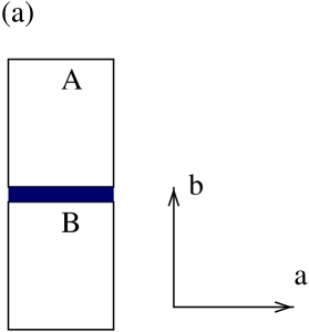
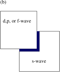
FIG. 1.: (a) A single Josephson junction between superconductors $A$ and $B$ with a two component order parameter. Also a small co-ordinate system indicating $a$ and $b$ crystalline directions is shown. (b) The geometry of the corner junction between a mixed symmetry superconductor and an $s$-wave superconductor.

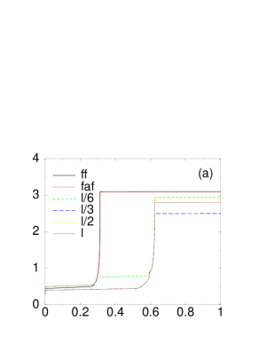
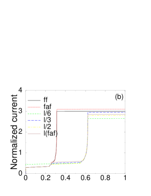
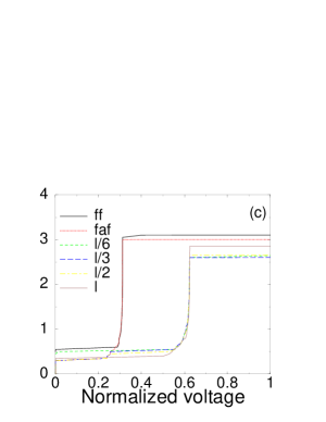
FIG. 2.: Normalized current versus the normalized voltage for the inline geometry, for the first and second ZFS. The solutions for the first ZFS are the $ff$, $faf$ corresponding to a bound fluxon or antifluxon in the junction’s center. For the second ZFS the solutions are labeled by the relative distance between the fluxons $l/x$, where $l=20$ is the junction length, and $x=1,2,3,6$ respectively, $\gamma=0.01$. The pairing state is (a) $B_{1g}$-wave, (b) $E_{u}$-wave, (c) $B_{1g}\times E_{u}$-wave.

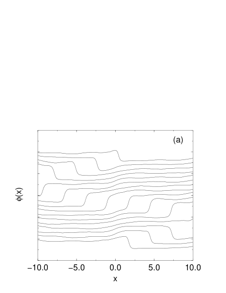
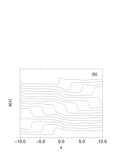
FIG. 3.: Phase $\phi(x)$ vs $x$ for the solutions in the first ZFS, at various instants, during one period separated by $\Delta\tau=2.8$. The curves are shifted by $0.5$ to avoid overlapping. $l=20$, $I=1.6$, $\gamma=0.01$: (a) $ff$, (b) $faf$. The pairing state is $B_{1g}$-wave.

FIG. 4.: Instantaneous voltage in the middle of the junction $(x=0)$ vs time $t$, for the solutions in the first ZFS. $l=20$, $\gamma=0.01$, $I=1.6$: (a) $ff$, (b) $faf$. The pairing state is $B_{1g}$-wave.

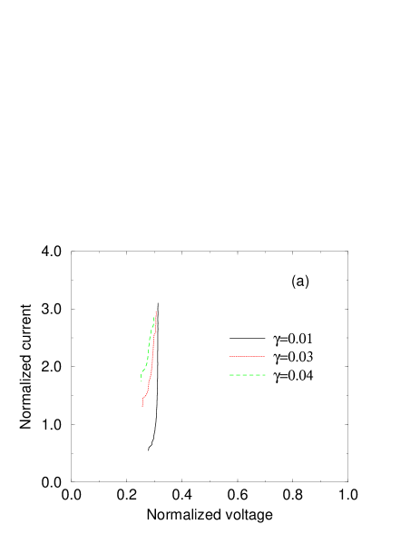
FIG. 5.: (a) Normalized current versus the normalized voltage for the inline geometry, for the $ff$ solution, for different values of the damping constant $\gamma$. $l=20$. The pairing state is $B_{1g}$-wave. (b) Instantaneous voltage in the middle of the junction $(x=0)$ vs time $t$, for the solution $ff$, $l=20$, $I=1.6$. The pairing state is $B_{1g}$-wave. The damping constant is $\gamma=0.03$.

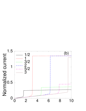
FIG. 6.: Normalized current versus the normalized voltage for the inline geometry, for a junction of length $l=2$, $\gamma=0.01$. The different modes are labeled by the value of the normalized voltage divided by $\pi$ in which they occur. The pairing state is (a) $B_{1g}$-wave, (b) $E_{u}$-wave, (c) $B_{1g}\times E_{u}$-wave.

FIG. 7.: Phase $\phi(x)$ vs $x$ for the solutions in the first three ZFS, at various instants, during one period separated by $\Delta\tau=0.2$. The pairing state is $B_{1g}$-wave. The curves are shifted by $0.5$ to avoid overlapping. $l=2$, $I=0.25$, $\gamma=0.01$.

FIG. 8.: Instantaneous voltage in the middle of the junction $(x=0)$ vs time $t$, for the solutions in the first three ZFS. The pairing state is $B_{1g}$-wave. $l=2$, $\gamma=0.01$, $I=0.25$.

REFERENCES

- [1] D.J. Scalapino, Phys. Rep. 250, 329 (1995).
- [2] D.J. Van Harlingen, Rev. Mod. Phys. 67, 515 (1995).
- [3] C.C. Tsuei and J.R. Kirtley, Rev. Mod. Phys. 72, 969 (2000).
- [4] N. Stefanakis and N. Flytzanis, Phys. Rev. B 61, 4270 (2000).
- [5] N. Stefanakis and N. Flytzanis, Phys. Rev. B 64, 024527 (2001).
- [6] N. Stefanakis, Phys. Rev. B 66, 024514 (2002).
- [7] Y. Maeno, H. Hashimoto, K. Yoshida, S. Nishizaki, T. Fujita, G.J . Bednorz and F. Lichtenberg, Nature 372, 532 (1994).
- [8] K. Ishida, H. Mukuda, Y. Kitaoka, K. Asayama, Z.Q. Mao, Y. Mori , and Y. Maeno, Nature 396, 658 (1998).
- [9] G.M. Luke, Y. Fukamoto, K.M. Kojima, M.L. Larkin, J. Merrin, B. N achumi, Y.J. Uemura, Y. Maeno, Z.Q. Mao, Y. Mori, H. Nakamura, and M. Sigrist, Nature 394, 558 (1998).
- [10] S. Nishizaki, Y. Maeno, and Z. Mao, J. Phys. Soc. Jpn. 69, 572 (2000).
- [11] N. Stefanakis, Phys. Rev. B 65, 064533 (2002).
- [12] T.A. Fulton and R.C. Dynes, Soild State Commum. 12, 57 (1973).
- [13] J.T. Chen, T.F. Finnegan and D.N. Langenberg, Physica 55, 413 (1971).
- [14] P.S. Lomdahl, O.H. Soerensen, and P.L. Christiansen, Phys. Rev. B 25, 5737 (1982).
- [15] I.V. Vernik, N. Lazarides, M.P. Sørensen, A.V. Ustinov, N.F. Pedersen, and V.A. Oboznov, J. Appl. Phys. 79, 7854 (1996).
- [16] A.B.Kuklov, V.S. Boyko, and J. Malinsky, Phys. Rev. B 51, 11 965 (1995).
- [17] T. Kato and M. Imada, J. Phys. Soc. Jpn. 66, 1445 (1997).
- [18] T.M. Rice and M. Sigrist, J. Phys.: Condens. Matter 7, L643 (1995)
- [19] Y. Hasegawa, K. Machida, and M. Ozaki, J. Phys. Soc. Jpn. 69, 336 (2000).
- [20] M. Scheuermann, J.R. Lhota, P.K. Kuo, and J.T. Chen, Phys. Rev. Lett. 50, 74 (1983).
- [21] L.B. Ioffe, V.B. Geshkenbein, M.V. Feigel’man, A.L. Fauchere, and G. Blatter, Nature 398, 679 (1999).
- [22] D.V. Averin, Solid State Commun. 105, 659 (1998).
- [23] F.W.J. Hekking, O. Buisson, F. Balestro, M.G. Vergniory, cond-mat/0201284, To appear in the Proceedings of the XXXVIth Rencontres de Moriond, January 2001, Les Arcs, France.
- [24] O. Bourgeois, P. Gandit, J. Lesueur, A. Sulpice, X. Grison, and J. Chaussy, Eur. Phys. J. B 21, 75 (2001).
- [25] T. Kontos, M. Aprili, J. Lesueur, F. Genet, B. Stephanidis, and R. Boursier, cond-mat/0201104.
- [26] R. Kleiner, F. Steinmeyer, G. Kunkel, and P. Müller , Phys. Rev. Lett. 68, 2394 (1992).