Coupled Replicator Equations for the
Dynamics of Learning in Multiagent Systems

Abstract

Starting with a group of reinforcement-learning agents we derive coupled replicator equations that describe the dynamics of collective learning in multiagent systems. We show that, although agents model their environment in a self-interested way without sharing knowledge, a game dynamics emerges naturally through environment-mediated interactions. An application to rock-scissors-paper game interactions shows that the collective learning dynamics exhibits a diversity of competitive and cooperative behaviors. These include quasiperiodicity, stable limit cycles, intermittency, and deterministic chaos—behaviors that should be expected in heterogeneous multiagent systems described by the general replicator equations we derive.

Adaptive behavior in multiagent systems is an important interdisciplinary topic that appears in various guises in many fields, including biology Camazine et al. (2001), computer science Simon (1996), economics Young (1998), and cognitive science Hutchins (1996). One of the key common questions is how and whether a group of intelligent agents truly engages in collective behaviors that are more functional than individuals acting alone.

Suppose that many agents interact with an environment and each independently builds a model from its sensory stimuli. In this simple type of coupled multiagent system, collective learning (if it occurs) is a dynamical behavior driven by agents’ environment-mediated interaction Rossler (1987); Taiji and Ikegami (1999). Here we show that the collective dynamics in multiagent systems, in which agents use reinforcement learning Sutton and Barto (1998), can be modeled using a generalized form of coupled replicator equations.

While replicator dynamics were introduced originally for evolutionary game theory Taylor and Jonker (1978), the relationship between reinforcement learning and replicator equations has been developed only recently Borgers and Sarin (1997). Here, we extend these considerations to multiagent systems, introducing the theory behind a previously reported game-theoretic model Sato et al., (2002). We show that replicator dynamics emerges as a special case of the continuous-time limit for multiagent reinforcement learning systems. The overall approach, though, establishes a general framework for dynamical-systems analyses of adaptive behavior in collectives.

Notably, in learning with perfect memory, our model reduces to the form of a multipopulation replicator equation introduced in Ref. Taylor (1979). For two agents with perfect memory interacting via a zero-sum rock-scissors-paper game the dynamics exhibits Hamiltonian chaos Sato et al., (2002). In contrast, as we show here, with memory decay multiagent systems generally become dissipative and display the full range of nonlinear dynamical behaviors, including limit cycles, intermittency, and deterministic chaos.

Our multiagent model begins with simple reinforcement learning agents. To simplify the development, we assume that there are two such agents $X$ and $Y$ that at each time step take one of $N$ actions: $i=1,\ldots,N$. Let the probability for $X$ to chose action $i$ be $x_{i}(n)$ and $y_{i}(n)$ for $Y$, where $n$ is the number of the learning iterations from the initial state at $n=0$. The agents’ choice distributions at time $n$ are ${\bf x}(n)=(x_{1}(n),\ldots,x_{N}(n))$ and ${\bf y}(n)=(y_{1}(n),\ldots,y_{N}(n))$, with $\Sigma_{i}x_{i}(n)=\Sigma_{i}y_{i}(n)=1$.

Let $R_{ij}^{X}$ and $R_{ij}^{Y}$ denote the reward for $X$ taking action $i$ and $Y$ action $j$ at step $n$, respectively. Given these actions, $X$’s and $Y$’s memories, $Q_{i}^{X}(n)$ and $Q_{i}^{Y}(n)$, of the past benefits from their actions are governed by

$$Q_{i}^{X}(n+1)-Q_{i}^{X}(n) = R_{ij}^{X}-\alpha_{X}Q_{i}^{X}(n)~{}{\rm and}$$ (1)

$$Q_{i}^{Y}(n+1)-Q_{i}^{Y}(n) = R_{ij}^{Y}-\alpha_{Y}Q_{i}^{Y}(n)~{},$$

where $\alpha_{X},\alpha_{Y}\in[0,1)$ control each agent’s memory decay rate and $Q_{i}^{X}(0)=Q_{i}^{Y}(0)=0$. The agents chose their next actions according to the $Q$’s, updating their choice distributions as follows:

$$x_{i}(n)=\frac{e^{\beta_{X}Q_{i}^{X}(n)}}{\Sigma_{j}e^{\beta_{X}Q_{j}^{X}(n)}}~{}{\rm and}~{}y_{i}(n)=\frac{e^{\beta_{Y}Q_{i}^{Y}(n)}}{\Sigma_{j}e^{\beta_{Y}Q_{j}^{Y}(n)}},$$ (2)

where $\beta_{X},\beta_{Y}\in[0,\infty]$ control the learning sensitivity: how much the current choice distributions are affected by past rewards. Using Eq. (2), the dynamic governing the change in agent state is given by:

$$x_{i}(n+1)=\frac{x_{i}(n)e^{\beta_{X}(Q_{i}^{X}(n+1)-Q_{i}^{X}(n))}}{\Sigma_{k}x_{j}(n)e^{\beta_{X}(Q_{k}^{X}(n+1)-Q_{k}^{X}(n))}}~{},$$ (3)

and similarly for $y_{i}(n+1)$.

Consider the continuous-time limit corresponding to agents performing a large number of actions (iterates of Eqs. (1)) for each choice-distribution update (iterates of Eq. (3)). In this case, we have two different time scales—that for agent-agent interactions and for learning. We assume that the learning dynamics is very slow compared to interactions and so $\bf x$ and $\bf y$ are essentially constant during the latter. Then, based on Eq. (3), continuous-time learning for agent $X$ is governed by

$$\dot{x}_{i}=\beta_{X}x_{i}(\dot{Q}_{i}^{X}-\Sigma_{j}\dot{Q}^{X}_{j}x_{j})~{},$$ (4)

and for the dynamic governing memory updates we have

$$\dot{Q}_{i}^{X}=R_{i}^{X}-\alpha_{X}Q_{i}^{X}~{},$$ (5)

where $R_{i}^{X}$ is the reward for $X$ choosing action $i$, averaged over $Y$’s actions during the time interval between learning updates. Putting together Eqs. (2), (4), and (5) one finds

$$\frac{\dot{x_{i}}}{x_{i}}=\beta_{X}[R_{i}^{X}-\Sigma_{j}x_{ij}R_{j}^{X}]+\alpha_{X}I^{X}_{i}~{},$$ (6)

where $I^{X}_{i}\equiv\Sigma_{j}x_{j}\log({x_{j}}/{x_{i}})$ represents the effect of memory with decay parameter $\alpha_{X}$. (The continuous-time dynamic of $Y$ follows in a similar manner.) Eq. (6), extended to account for any number of agents and actions, constitutes our general model for reinforcement-learning multiagent systems.

Simplifying again, assume a fixed relationship between pairs $(i,j)$ of $X$’s and $Y$’s actions and between rewards for both agents: $R_{ij}^{X}=a_{ij}$ and $R_{ij}^{Y}=b_{ij}$. Assume further that $\bf x$ and $\bf y$ are independently distributed, then the time-average rewards for $X$ and $Y$ become

$$R_{i}^{X}=\Sigma_{j}a_{ij}y_{j}~{}{\rm and}~{}R_{i}^{Y}=\Sigma_{j}b_{ij}x_{j}~{},$$ (7)

In this restricted case, the continuous-time dynamic is:

$$\frac{\dot{x}_{i}}{x_{i}} = \beta_{X}[(A{\bf y})_{i}-{\bf x}\cdot A{\bf y}]+\alpha_{X}I^{X}_{i}~{},$$

$$\frac{\dot{y}_{i}}{y_{i}} = \beta_{Y}[(B{\bf x})_{i}-{\bf y}\cdot B{\bf x}]+\alpha_{Y}I^{Y}_{i}~{},$$ (8)

where $(A)_{ij}=a_{ij}$ and $(B)_{ij}=b_{ij}$, $(A{\bf x})_{i}$ is the $i$th element of the vector $A{\bf x}$, and $\beta_{X}$ and $\beta_{Y}$ control the time-scale of each agent’s learning.

We can regard $A$ and $B$ as $X$’s and $Y$’s game-theoretic payoff matrices for action $i$ against opponent’s action $j$ . In contrast with game theory, which assumes agents have exact knowledge of the game structure and of other agent’s strategies, reinforcement-learning agents have no knowledge of a “game” in which they are playing, only a myopic model of the environment—other agent(s)—given implicitly via the rewards they receive. Nonetheless, a game dynamics emerges—via $R^{X}$ and $R^{Y}$ in Eq. (6)—as a description of the collective’s global behavior.

Given the basic equations of motion for the reinforcement-learning multiagent system (Eq. (8)), one becomes interested in, on the one hand, the time evolution of each agent’s state vector in the simplices ${\bf x}\in\Delta_{X}$ and ${\bf y}\in\Delta_{Y}$ and, on the other, the dynamics in the higher-dimensional collective simplex $({\bf x},{\bf y})\in\Delta_{X}\times\Delta_{Y}$. Following Ref. Hofbauer (1996), we transform from $({\bf x},{\bf y})\in\Delta_{X}\times\Delta_{Y}$ to ${\bf U}=({\bf u},{\bf v})\in{\bf R}^{2(N-1)}$ with ${\bf u}=(u_{1},\ldots,u_{N-1})$ and ${\bf v}=(v_{1},\ldots,v_{N-1})$, where $u_{i}=\log(x_{i+1}/x_{1})~{}{\rm and}~{}v_{i}=\log(y_{i+1}/y_{1}),~{}(i=1,\ldots,N-1)$. The result is a new version of our simplified model (Eqs. (8)), useful both for numerical stability during simulation and also for analysis in certain limits:

$$\dot{u}_{i} = \beta_{X}\frac{\Sigma_{j}\tilde{a}_{ij}e^{v_{j}}+\tilde{a}_{i1}}{1+\Sigma_{j}e^{v_{j}}}-\alpha_{X}u_{i}~{}{\rm and}$$

$$\dot{v}_{i} = \beta_{Y}\frac{\Sigma_{j}\tilde{b}_{ij}e^{u_{j}}+\tilde{b}_{i1}}{1+\Sigma_{j}e^{u_{j}}}-\alpha_{Y}v_{i}~{},$$ (9)

where $\tilde{a}_{ij}=a_{i+1,j}-a_{1,j}$ and $\tilde{b}_{ij}=b_{i+1,j}-b_{1,j}$. Since the dissipation rate $\gamma$ in $\bf U$ is

$$\gamma=\Sigma_{i}\frac{\partial\dot{u}_{i}}{\partial u_{i}}+\Sigma_{j}\frac{\partial\dot{v}_{j}}{\partial v_{j}}=-(N-1)(\alpha_{X}+\alpha_{Y}),$$ (10)

Eqs. (8) are conservative when $\alpha_{X}=\alpha_{Y}=0$ and the time average of a trajectory is the Nash equilibrium of the game specified by $A$ and $B$, if a limit set exists in the interior of $\Delta_{X}\times\Delta_{Y}$. Moreover, if the game is zero-sum, the dynamics are Hamiltonian in ${\bf U}$ with

$$H = -(\Sigma_{j}x^{*}_{j}u_{j}+\Sigma_{j}y^{*}_{j}v_{j})$$

$$+ \log(1+\Sigma_{j}e^{u_{j}})+\log(1+\Sigma_{j}e^{v_{j}})~{},$$

where $({\bf x}^{*},{\bf y}^{*})$ is an interior Nash equilibrium Hofbauer (1996).

To illustrate the dynamical-systems analysis of learning in multiagent systems using the above framework, we now analyze the behavior of the two-person rock-scissors-paper interaction . This familiar game describes a nontransitive three-sided competition: rock beats scissors, scissors beats paper, and paper beats rock. The reward structure (environment) is given by:

$$A=\left[\begin{array}[]{ccc}\epsilon_{X}&1&-1\\ -1&\epsilon_{X}&1\\ 1&-1&\epsilon_{X}\\ \end{array}\right]~{}{\rm and}~{}B=\left[\begin{array}[]{ccc}\epsilon_{Y}&1&-1\\ -1&\epsilon_{Y}&1\\ 1&-1&\epsilon_{Y}\\ \end{array}\right]~{},$$ (12)

where $\epsilon_{X},\epsilon_{Y}\in[-1.0,1.0]$ are the rewards for ties. The mixed Nash equilibrium is $x^{*}_{i}=y^{*}_{i}=1/3,(i=1,2,3)$—the centers of $\Delta_{X}$ and $\Delta_{Y}$. If $\epsilon_{X}=-\epsilon_{Y}$, the game is zero-sum.

In the special case of perfect memory ($\alpha_{X}=\alpha_{Y}=0$) and with equal learning sensitivity ($\beta_{X}=\beta_{Y}$), the linear version (Eqs. (8)) of our model (Eq. (6)) reduces to multipopulation replicator equations Taylor (1979):

$$\frac{\dot{x}_{i}}{x_{i}}=\left[(A{\bf y})_{i}-{\bf x}\cdot A{\bf y}\right]~{}{\rm and}~{}\frac{\dot{y}_{i}}{y_{i}}=\left[(B{\bf x})_{i}-{\bf y}\cdot B{\bf x}\right]~{}.$$ (13)

Figure 1: Quasiperiodic tori and chaos: $\epsilon_{X}=-\epsilon_{Y}=0.5$, $\alpha_{X}=\alpha_{Y}=0$, and $\beta_{X}=\beta_{Y}$. We give a Poincaré section (top) on the hyperplane defined by $\dot{u}_{1}=0$ and $\dot{v}_{1}>0$; that is, in the $({\bf x},{\bf y})$ space: $(3+\epsilon_{X})y_{1}+(3-\epsilon_{X})y_{2}-2=0$ and $(3+\epsilon_{Y})x_{1}+(3-\epsilon_{Y})x_{2}-2<0$. There are 23 randomly selected initial conditions with energies $H=-1/3(u_{1}+u_{2}+v_{1}+v_{2})+\log(1+e^{u_{1}}+e^{u_{2}})+\log(1+e^{v_{1}}+e^{v_{2}})=2.941693$, which surface forms the outer border of $H\leq 2.941693$. Two rows (bottom): Representative trajectories, simulated with a $4$th-order symplectic integrator Yoshida (1990), starting from initial conditions within the Poincaré section. The upper simplices show a torus in the section’s upper right corner; see the enlarged section at the upper right. The initial condition is $({\bf x},{\bf y})=(0.3,0.054196,0.645804,0.1,0.2,0.7)$. The lower simplices are an example of a chaotic trajectory passing through the regions in the section that are a scatter of dots; the initial condition is $({\bf x},{\bf y})=(0.05,0.35,0.6,0.1,0.2,0.7)$.

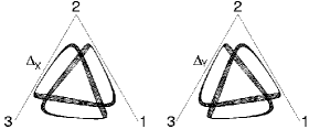
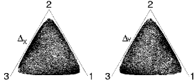
The game-theoretic behavior in this case with rock-scissors-paper interactions (Eqs. (12)) was investigated in Sato et al., (2002). Here, before contrasting our more general setting, we briefly recall the behavior in these special cases, noting several additional results.

Figure 1 shows Poincaré sections of Eqs. (13)’s trajectories on the hyperplane $(\dot{u}_{1}=0,\dot{v}_{1}>0)$ and representative trajectories in the individual agent simplices $\Delta_{X}$ and $\Delta_{Y}$. When $\epsilon_{X}=-\epsilon_{Y}=0.0$, we expect the system to be integrable and only quasiperiodic tori should exist. Otherwise, $\epsilon_{X}=-\epsilon_{Y}>0.0$, Hamiltonian chaos can occur with positive-negative pairs of Lyapunov exponents Sato et al., (2002). The dynamics is very rich, there are infinitely many distinct behaviors near the unstable fixed point at the center—the classical Nash equilibrium—and a periodic orbit arbitrarily close to any chaotic one. Moreover, when the game is not zero-sum ($\epsilon_{X}\neq\epsilon_{Y}$), transients to heteroclinic cycles are observed Sato et al., (2002): On the one hand, there are intermittent behaviors in which the time spent near pure strategies (the simplicial vertices) increases subexponentially with $\epsilon_{X}+\epsilon_{Y}<0$ and, on the other hand, with $\epsilon_{X}+\epsilon_{Y}>0$, chaotic transients persist; cf. Chawanya (1995).

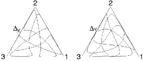
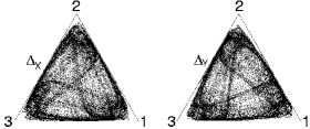
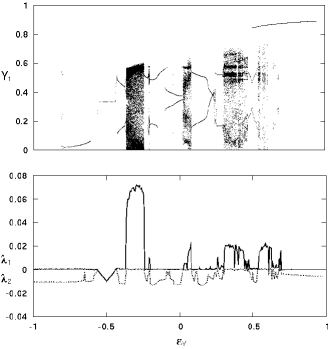
Our framework goes beyond these special cases and, generally, beyond the standard multipopulation replicator equations (Eqs. (13)) due to its accounting for the effects of individual and collective learning and since the reward structure and the learning rules need not lead to linear interactions. For example, if the memory decay rates ($\alpha_{X}$ and $\alpha_{Y}$) are positive, the system becomes dissipative and exhibits limit cycles and chaotic attractors; see Fig. 2. Figure 3 (top) shows a diverse range of bifurcations as a function of $\epsilon_{Y}$: dynamics on the hyperplane ($\dot{u}_{1}=0$, $\dot{v}_{1}>0$) projected onto $y_{1}$. When the game is nearly zero-sum, agents can reach the stable Nash equilibrium, but chaos can also occur, when $\epsilon_{X}+\epsilon_{Y}>0$. Figure 3 (bottom) shows that the largest Lyapunov exponent is positive across a significant fraction of parameter space; indicating that chaos is common. The dual aspects of chaos, irregularity and coherence, imply that agents may behave cooperatively or competitively (or switch between both) in the collective dynamics. Such global behaviors ultimately derive from self-interested, myopic learning.

Figure 2: Limit cycle (top: $\epsilon_{Y}=0.025$) and chaotic attractors (bottom: $\epsilon_{Y}=-0.365$), with $\epsilon_{X}=0.5$, $\alpha_{X}=\alpha_{y}=0.01$, and $\beta_{X}=\beta_{Y}$.

Figure 3: Bifurcation diagram (top) of dissipative (learning with memory loss) dynamics projected onto coordinate $y_{1}$ from the Poincaré section hyperplane ($\dot{u}_{1}=0$, $\dot{v}_{1}>0$) and the largest two Lyapunov exponents $\lambda_{1}$ and $\lambda_{2}$ (bottom) as a function of $\epsilon_{Y}\in[-1,1]$. Here with $\epsilon_{X}=0.5$, $\alpha_{X}=\alpha_{Y}=0.01$, and $\beta_{X}=\beta_{Y}$. Simulations show that $\lambda_{3}$ and $\lambda_{4}$ are always negative.

Within this framework a number of extensions suggest themselves as ways to investigate the emergence of collective behaviors. The most obvious is the generalization to an arbitrary number of agents with an arbitrary number of strategies and the analysis of behaviors in thermodynamic limit; see, e.g., Marsili et al. (2000) as an alternative approach. It is relatively straightforward to develop an extension to the linear-reward version (Eqs. (8)) of our model. For three agents $X$, $Y$, and $Z$, one obtains:

$$\frac{\dot{x}_{i}}{x_{i}}=\beta_{X}[\Sigma_{j,k}a_{ijk}y_{j}z_{k}-\Sigma_{j,k,l}a_{jkl}x_{j}y_{k}z_{l}]-\alpha_{X}I_{i}^{X}~{},$$ (14)

with tensor $(A)_{ijk}=a_{ijk}$, and similarly for $Y$ and $Z$. Not surprisingly, this is also a conservative system when the $\alpha$’s vanish. However, extending the general collective learning equations (Eq. (6)) to multiple agents is challenging and so will be reported elsewhere.

To be relevant to applications, one also needs to develop a statistical dynamics generalization van Nimwegen et al. (1999) of the deterministic equations of motion to account for finite and fluctuating numbers of agents and also finite histories used in learning. Finally, another direction, especially useful if one attempts to quantify collective function in large multiagent systems, will be structural and information-theoretic analyses Crutchfield and Young (1989) of local and global learning behaviors and, importantly, their differences. Analyzing the stored information in each agent versus that in the collective, the causal architecture of information flow between an individual agent and the group, and how individual and global memories are processed to sustain collective function are projects now made possible using this framework.

We presented a dynamical-systems model of collective learning in multiagent systems, which starts with reinforcement learning agents and reduces to coupled replicator equations, demonstrated that individual-agent learning induces a global game dynamics, and investigated some of the resulting periodic, intermittent, and chaotic behaviors with simple (linear) rock-scissors-papers game interactions. Our model gives a macroscopic description of a network of learning agents that can be straightforwardly extended to model a large number of heterogeneous agents in fluctuating environments. Since deterministic chaos occurs even in this simple setting, one expects that in high-dimensional and heterogeneous populations typical of multiagent systems intrinsic unpredictability will become a dominant collective behavior. Sustaining useful collective function in multiagent systems becomes an even more compelling question in light of these results.

The authors thank J. D. Farmer, E. Akiyama, P. Patelli, and C. Shalizi. This work was supported at the Santa Fe Institute under the Network Dynamics Program by Intel Corporation and under DARPA agreement F30602-00-2-0583. YS’s participation was supported by the Postdoctoral Researchers Program at RIKEN.

References

- Camazine et al. (2001) S. Camazine et al eds., Self-Organization in Biological Systems (Princeton University Press, 2001).
- Simon (1996) H. A. Simon, The Sciences of the Artificial, Karl Taylor Compton Lectures (MIT Press, 1996).
- Young (1998) H. P. Young, Individual strategy and Social Structure (Princeton University Press, 1998).
- Hutchins (1996) E. Hutchins, Cognition in the Wild (MIT Press, 1996).
- Rossler (1987) O. E. Rossler, Ann. NY Acad, Sci. 504, 229 (1987).
- Taiji and Ikegami (1999) M. Taiji and T. Ikegami, Physica D 134, 253 (1999).
- Sutton and Barto (1998) R. S. Sutton and A. G. Barto, Reinforcement learning: An introduction (MIT Press, 1998).
- Taylor and Jonker (1978) P. Taylor and L. Jonker, Math. Bio. 40, 145 (1978).
- Borgers and Sarin (1997) T. Borgers and R. Sarin, J. Econ. Th. 77, 1 (1997).
- Taylor (1979) P. Taylor, J. Appl. Prob. 16, 76 (1979).
- Hofbauer (1996) J. Hofbauer, J. Math. Biol. 34, 675 (1996).
- Yoshida (1990) H. Yoshida, Phys. Lett. A 150, 262 (1990).
- Sato et al., (2002) Y. Sato, E. Akiyama, and J. D. Farmer, Proc. Natl. Acad. Sci. USA 99, 4748 (2002).
- Chawanya (1995) T. Chawanya, Prog. Theo. Phys. 94, 163 (1995).
- Marsili et al. (2000) M. Marsili, D. Challet and R. Zecchina, Physica A 280, 522 (2000).
- van Nimwegen et al. (1999) E. van Nimwegen, J. P. Crutchfield, and M. Mitchell, Theor. Comp. Sci. 229, 41 (1999).
- Crutchfield and Young (1989) J. P. Crutchfield and K. Young, Phys. Rev. Lett. 63, 105 (1989), see also, arXiv.org/abs/cond-mat/0102181.