Structure of Rule Table and Phase Diagram of One Dimensional Cellular Automata

Abstract

In addition to the $\lambda$ parameter, we have found another parameter which characterize the class III, class II and class IV patterns more quantitatively. It explains why the different classes of patterns coexist at the same $\lambda$. With this parameter, the phase diagram for an one dimensional cellular automata is obtained. Our result explains why the edge of chaos(class IV) is scattered rather wide range in $\lambda$ around $0.5$, and presents an effective way to control the pattern classes.

1 Introduction

The study of the cellular automata(CA) has been one of the most important fields for the understanding of the complex systems. And many efforts have been carried out for the understanding of it. Various patterns had been generated by choosing the transition rules, and the patterns have been classified by Wolfram roughly into four classes[1]. Langton has introduced parameter $\lambda$ and showed that as $\lambda$ is increased the pattern changes from class I(homogeneous),class II(periodic) to class III(chaotic). And at some cases, the class IV(edge of chaos) is realized between the two[2, 3].

The $\lambda$ parameter could classify the qualitative behavior of the CA, but it is not enough[4]. It is well known that at the same $\lambda$ the time evolution of the configuration shows periodic pattern(class II), chaotic one(class III) or edge of the chaos pattern(class IV) depending on the initial seed of the random number generator. The reason or mechanism for it has not been known yet; we have no way to control the pattern classes at fixed $\lambda$. And the transition of periodic to chaotic pattern is taken place at rather wide range of $\lambda$. Therefore it is a natural anticipation that more parameters are necessary to get the quantitative understanding of the pattern classes of the CA. In this article we report another parameter which classifies the pattern classes more quantitatively. If the capacity to support computation is realized at the edge of the chaos[2, 4], we have acquired a method to reach there more effectively.

In the section 2, we will briefly summarize our notations and explain the key discovery which leads us to the understanding of the structure of the rule table. It strongly indicates that the rules which destroy the schema of the quiescent state play an important role to distinguish the pattern classes.

In the section 3, guided by the discovery of the section 2, we classify the rule table according to the destruction and construction of the schema of the quiescent states. The rule which destroys the longest schema of the quiescent state plays strongest effects for the patterns. Then we introduce a new parameter force for each rules which destroy the schema. With this parameter, we determine the phase diagram in the $\lambda$ and the force plane. It clearly explains why at fixed $\lambda$ the different patterns are generated and we could control the pattern classes more quantitatively.

Section 4 is devoted to the discussions and the conclusions, where effects of the structure of the rule table will further be discussed.

2 Discovery of the Key Rules

2.1 Summary of the Notation

In order to make the argument concrete, in this article we focus on the one dimensional cellular automata with 5-neighbors and 4-states. But the qualitative results are independent of the details of the models. This point will be discussed in section 4. We follow the definitions of Langton[2] but for the self consistentness we will briefly summarize them.

In our study, the sites consist of 150 cells with the periodic boundary condition, which are denoted as $s(t,i)$. The $t$ represents the time step which take integer value, and the $i$ is the position of site which range from $0$ to $149$. The $s(t,i)$ takes the value $0,1,2$ and $3$, and the state $0$ is taken to be quiescent state[2]. The set of the states $s(t,i)$ at fixed $t$ is called the configuration at time $t$.

The configuration at time $t+1$ is determined by that of time $t$ by the following local relation,

$$s(t+1,i)=T(s(t,i-2),s(t,i-1),s(t,i),s(t,i+1),s(t,i+2))$$ (1)

The set of the mappings

$$T(\mu,\nu,\kappa,\rho,\sigma)=\eta,(\mu,\nu,etc=0,1,2,3)$$ (2)

is called rule table. The rule table consists of $4^{5}$ mappings, which are selected from the totally $4^{1024}$ elements.

The $\lambda$ parameter is defined as follows[2],

$$\lambda=\frac{N_{h}}{1024}$$ (3)

where $N_{h}$ is the number that $\eta$ in Eq.2 is not equal to $0$. In other word the $\lambda$ is a probability that the rules do not select the quiescent state in next time step. In the following we set the rule tables randomly according to the probability $\lambda$[2], and the initial configurations are also set randomly.

The time history of the configurations is called pattern. The patterns are classified by Wolfram[1] roughly into four classes. It has been known that as the $\lambda$ increases the most frequently generated patterns change from homogeneous(class I), periodic(class II) to chaotic(class III) and at the region between class II and class III, the edge of chaos is located(class IV).

2.2 Experiments at $\lambda=0.44$ and Discovery of the Key Rule

In order to find the reason why the different patterns are generated at the same $\lambda$, we had started to collect a lot of rule tables with different pattern classes. And by studying them, we had tried to find the differences between rule tables. We had fixed $N_{h}=455$, which correspond to $\lambda=0.44$. We had chosen this $\lambda$ because at this point the chaotic, edge of chaos and periodic patterns are generated in the similar ratio. By changing the random number, we have gathered a few tens of the rule tables and classified them into chaotic, edge of chaos and periodic ones.

First we studied whether the pattern classes are sensitive to the initial configurations or not. We fixed the rule table and changed the initial configurations. The details of the patterns depend on the initial configurations but the pattern classes are not changed[1]. Then the difference of the pattern classes is due to that of the rule tables and our target is addressed to the study of them.

After some trial and error, we have found the fact that for rule tables which generate the edge of the chaos and periodic patterns, the transition table $T(0,0,0,0,0)$ was almost always equal to $0$, while for that of the chaotic pattern, it was not equal to $0$ in majority of cases. For about 10 rule tables of each pattern classes, we get following results for the probability that the rule tables have $T(0,0,0,0,0)=0$.

$$Prob(T(0,0,0,0,0)=0)\sim 1$$ (4)

for periodic plus edge of chaos rule tables,

$$Prob(T(0,0,0,0,0)=0)\sim 0.2$$ (5)

for chaotic rule tables.

In this article, we call the pattern as edge of chaos when its transient length[2] is longer than $3000$ time steps.

These difference given by Eq.4 and Eq.5 has lead us the following idea. Let us think of the schemas of quiescent state $0$ with length longer than five. If the rule $T(0,0,0,0,0)=h,(h\neq 0)$ is included in the rule table, they are necessarily broken . Then it pushes the pattern to that of chaos.

If our idea is correct, we could artificially change the rule tables of the chaos to that of periodic by replacing $T(0,0,0,0,0)=h$ to $T(0,0,0,0,0)=0$. We have tried the replacements for about 10 rule tables. In all cases we have succeeded to change the rule tables from chaotic to periodic or periodic to chaotic by a replacements of the $T(0,0,0,0,0)$. An example is shown in the Figure 1. The change in the pattern is dramatical but the differences in the rule table are only two, which has been quite exciting for us.

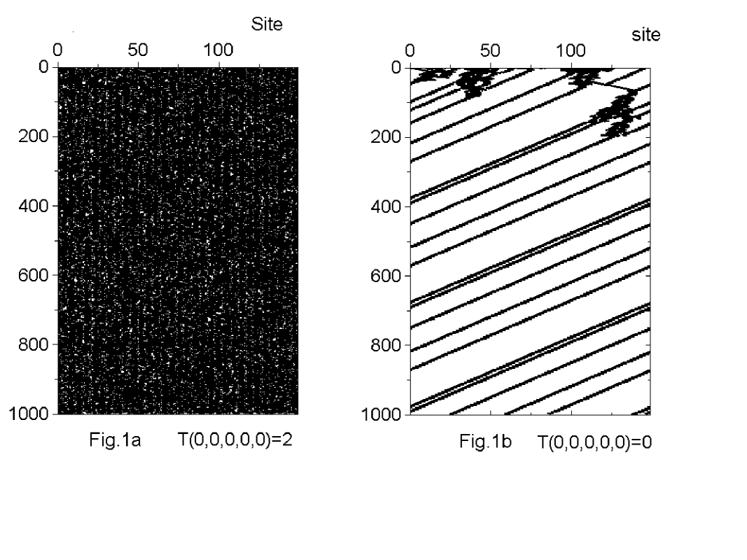
Figure 1: An example of the replacements experiment at $\lambda=0.44$. The quiescent state is shown with white points and the other states, with black one. The rule $T(0,0,0,0,0)=2$ in the Fig.1a is replaced by $T(0,0,0,0,0)=0$ in the Fig.1b, and at the same time a replacement $T(\mu,\nu,k,\rho,\sigma)=0,(k\neq 0)\rightarrow T(\mu,\nu,k,\rho,\sigma)=l,(l\neq 0)$ has been carried out to keep the $\lambda$ unchanged.

This discovery was a key hint to lead us to the hypothesis that the rules which breaks the schema of the quiescent state will determine the pattern classes.

3 Structure of Rule Table and Phase Diagram

3.1 Classification of the Rule Table

In order to test the hypothesis of the previous section, we group the rule table into the four types according to the operation on the schema of quiescent state.

In the following, Greek characters in the rule table represent $0,1,2$ and $3$ while Roman ones $1,2$ and $3$.

Type 1: $T(\mu,\nu,0,\rho,\sigma)=h$.
The rules in this type destroy the schemas of quiescent state.

Type 2: $T(\mu,\nu,0,\rho,\sigma)=0$.
The rules of this type conserve them.

Type 3: $T(\mu,\nu,k,\rho,\sigma)=0$.
The rules of this type develop the schema.

Type 4: $T(\mu,\nu,k,\rho,\sigma)=l$.
The rules in this type do not affect the schema in next time step.

The sum of the number of the type 1 and type 2 rules is 256, while that of type 3 and type 4 rules is 768. How many numbers of each type of rules are included in the rule table is determined randomly according to the probability $\lambda$.

The type 1 rules are further classified into five groups according to the length of the schema which breaks. They are shown in the Table 1.

group	Total Number	Name	Replacement
$T(0,0,0,0,0)=h$	1	D5	RP5
$T(0,0,0,0,i)=h$	3	D4	RP4
$T(i,0,0,0,0)=h$	3
$T(0,0,0,i,\sigma)=h$	12
$T(i,0,0,0,m)=h$	9	D3	RP3
$T(\mu,j,0,0,0)=h$	12
$T(\mu,j,0,0,m)=h$	36	D2	RP2
$T(i,0,0,l,\sigma)=h$	36
$T(\mu,j,0,l,\sigma)=h$	144	D1	RP1

Table 1: The classification of the rules in type 1.

Our hypothesis presented at the end of the previous section is expressed more quantitatively as follows; what groups of rules and how many of them shown in the table 1 are included in the rule table will determine whether the resulting patterns become chaotic, edge of chaos, or periodic.

In order to test this hypothesis we have artificially replaced some of the rules in the table 1 while keeping the $\lambda$ fixed. For the D5, it is a set of the replacements given by the following equations, which are already carried out in obtaining Fig.1.

$$\begin{array}[]{ll}T(0,0,0,0,0)=h\rightarrow T(0,0,0,0,0)=0\\ T(\mu,\nu,k,\rho,\sigma)=0\rightarrow T(\mu,\nu,k,\rho,\sigma)=l\\ \end{array}$$ (6)

where except for $h$, the $\mu$, $\nu$, $\rho$, $\sigma$, $k$ and $l$ are selected randomly.

Similarly the replacements are generalized for D4 to D1 in the table 1, which are named by RP5 to RP1 there. They change the rules in type 1 to that of the type 2 and push the rule table toward periodic one.

The reverse replacements for D5 are,

$$\begin{array}[]{ll}T(0,0,0,0,0)=0\rightarrow T(0,0,0,0,0)=h\\ T(\mu,\nu,k,\rho,\sigma)=l\rightarrow T(\mu,\nu,k,\rho,\sigma)=0\\ \end{array}$$ (7)

which push the rule table toward chaotic one. In this case $h$ is selected randomly, while $l$ is fixed in rule table. Similarly we define the replacements for D4 to D1, which will be called RC5 to RC1 in the followings.

We have made replacements RP5 to RP1 if the initial rule table generates chaotic pattern and RC5 to RC1 if it belongs to the periodic rules. These replacement experiments are carried out for $\lambda=0.6$,$0.5$ and $0.4$.

When the replacements include RP5, a few additional replacements RP4s together with D5 make the chaotic pattern to periodic ones and converse is true for the RC5. The numbers of the replacements needed to change the pattern are alway less than the $1\%$ of the $1024$ elements of the rule tables.

When the replacement does not include RP5 or RC5 the number of the replacement needed to change the pattern classes increases. This means that the effects to push the rule table toward periodic are different for the replacements in table 1. From a few tens of the replacements experiments the following order for the effects are observed.

$$RP5>RP4>RP3>RP2>RP1$$ (8)

3.2 Phase Diagram in Term of Force of Type 1 Rules

In order to make the relation given by Eq. 8 more quantitative we introduce a new parameter force for type 1 rules.

We assume that each rule in the table 1 have their own force to push the rule tables toward the chaos. The force may be a complicated function of the numbers of type 1 to type 4 rules, or it may even depend on the detailed contents of the 1024 rules. But as a first approximation, we take that it depends only on numbers of the rules D5, D4, D3, D2 and D1 in table 1, which are denoted as $N_{5}$, $N_{4}$, $N_{3}$, $N_{2}$ and $N_{1}$ respectively.

Second we assume that the forces are represented by the simple weighted sum of the number $N_{5}$ to $N_{1}$. The weight represents the strength of the force and expressed by the coefficients $c_{5}$ to $c_{1}$.

In the study of the replacement of the rule tables, we found that the D1 has quite small force to change the rule table. In some cases the replacement RP1 pushes the rules to chaotic one. In these cases it is close to the random walk in the rule table space and the determination of $c_{1}$ needs much statistics. In the following we neglect the contribution from D1 rule and set $c_{1}=0$ as a first approximation. Then the force is given as follows .

$$f(N_{5},N_{4},N_{3},N_{2})=c_{5}N_{5}+c_{4}N_{4}+c_{3}N_{3}+c_{2}N_{2}$$ (9)

The ansatz given in Eq. 9 is a first step to the more detailed study of the structure of rule tables of the CA. The fine forces of D2 or even by the D3 may depend on the fine structure of the type 3 and type 4 rules. In this article these details are neglected.

By artificially carrying out the replacements of RP5 to RP2 or RC5 to RC2 we look for the critical combinations of the $N_{5}$ to $N_{2}$, where the change of the patterns is observed. We have collected about 60 to 85 sets of critical combinations for each $\lambda$. We assume that the transition occurs when the force given by Eq.9 exceeds at some fixed threshold value. The threshold value is not known a priori and it may depend on the individual rule table, but as a first approximation, we assume that it is common for a given $\lambda$. With this condition, we proceed to determine the coefficients.

However in this condition the scale for the force is arbitrary. We measure it in the unit where force from D5 is equal to one, which correspond to divide the force in Eq. 9 by $c_{5}$ and express it as the ratio $r_{4}$, $r_{3}$ and $r_{2}$, where $r_{4}=\frac{c_{4}}{c_{5}}$, similarly for $r_{3}$ and $r_{2}$. Then our problem is to find the $r_{4}$, $r_{3}$ and $r_{2}$, which minimize the following quantity,

$$s(r_{4},r_{3},r_{2})=\frac{1}{c_{5}^{2}}\sum_{i,j}(f^{i}(N_{5}^{i},N_{4}^{i},N_{3}^{i},N_{2}^{i})-f^{j}(N_{5}^{j},N_{4}^{j},N_{3}^{j},N_{2}^{j}))^{2}$$ (10)

The results for $r_{4}$, $r_{3}$ and $r_{2}$ are given in the table 2, where the errors are estimated by jackknife method. They satisfy the order given by the Eq.8. This shows a hierarchy in the forces of the rules in table 1.

$\lambda$		Relative Strength	Error
	$r_{4}$	0.1126	0.0034
$\lambda=0.4$	$r_{3}$	0.0418	0.0013
	$r_{2}$	0.0109	0.0053
	$r_{4}$	0.1230	0.0046
$\lambda=0.5$	$r_{3}$	0.0432	0.0014
	$r_{2}$	0.0119	0.0012
	$r_{4}$	0.1138	0.0026
$\lambda=0.6$	$r_{3}$	0.0275	0.0034
	$r_{2}$	0.0201	0.0012

Table 2: The relative strength of forces for the groups of rules given by the table 1.

The results in table 2 are natural in the following sense. If six D4 rules are present for the rule table, then the presence of D5 has no effects, because the length 5 schema of quiescent state could not be made. They have roughly similar effects as one D5 rule, then the strength of the D4 will approximately be equal to $1/6$ of that of D5. Similarly the strength of the D3 and D2 will be about $1/33$ and $1/72$ respectively. The results given in the table 2 are not very different from these naive expectations.

With these results for the coefficients of Eq.9, we determine the transition points by means of the force. We call it as critical force($f_{critical}$). The results are shown in the Fig.2. In the Fig.2, we have added $f_{critical}/c_{5}$ calculated from the naive expectations for the relative strengths. In this case too, errors are estimated by the jackknife method. The difference between them are not large.

This figure distinguishes the pattern classes more quantitatively, and visualizes why at the fixed $\lambda$ the three patterns chaos, edge of the chaos and periodic coexist.

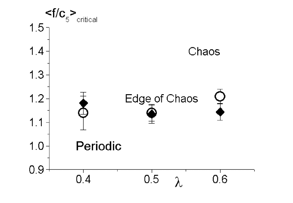
Figure 2: Phase diagram of the 5-Neighbor 4-State cellular Automata. The open circle is the $f_{critical}/c_{5}$ from the relative strength of the table 2, while the filled diamond show the $f_{critical}/c_{5}$ from the naive expectations discussed in the text. We should like to notice that force is divided by $c_{5}$, which may depends on $\lambda$.

The impressive point is that the transition occurs about $f/c_{5}\sim 1.14-1.2$. This means that in many cases the replacements of D5 will change the pattern classes, which is consistent with the experiments at section 2.

We should like to notice that the phase diagram shown in Fig. 2 is an average over about 60 to 85 sets of the critical combinations, which belong to different rule tables.

4 Discussions and Conclusions

$\odot$ Difference of Patterns with $T(0,0,0,0,0)=h$ and $T(0,0,0,0,0)=0$

By carrying out the replacements RP4s and RP3s, we could artificially obtain the rule table of periodic pattern with $T(0,0,0,0,0)=h$. In this case the length of the schema of quiescent state could not develop longer than 4, then the patterns will have thin stripes in the time direction. While for the patterns generated by the rule table without D5, there is very small probability that the thin stripes are created. Then there will be clear difference between the two patterns. An example is shown in the Fig.3. The differences in patterns is again dramatical while those in rule table are only 2.

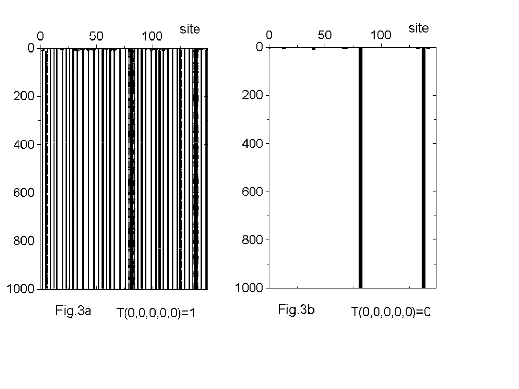
Figure 3: The difference of the patterns with and without the rule $T(0,0,0,0,0)=0$ at $\lambda=0.4$. The rule $T(0,0,0,0,0)=1$ in the Fig.3a is replaced by $T(0,0,0,0,0)=0$ in the Fig.3b;the RP5 is carried out.

Similarly for the patterns of an edge of the chaos, when the rule tables have D5, the patterns are drawn on the background of the thin stripes as shown in the Fig.3a, while if they do not include D5, patterns are drawn essentially on the quiescent states. The differences between these two patterns are impressive. Similar situation is observed for the pattern when six D4s are included in the rule table. In this case, the maximum length of the schema of quiescent state is 3, that the width of the stripe becomes more narrow. The existence of the rules of the table 1 has strong effects for the details of the patterns.

$\odot$ Fluctuation of Rule Tables around $\lambda\sim 0.5$

When the rule tables are generated randomly, how many type 1 rules are included, is determined randomly by the probability $\lambda$. The largest fluctuation is realized for D5, because it has only one element. Next is D4 and so on. And the transition is taken place about $1.14$ to $1.2$ of the force expressed in the unit of $c_{5}$. Then the change of the pattern classes are easily realized by the fluctuation of $N_{5}$ and $N_{4}$ at fixed $\lambda$. This fact explains why the transition and edge of chaos is scattered rather wide range in $\lambda$.

Also the fluctuation is largest at $\lambda=0.5$. Then the coexistence of the periodic pattern and chaotic pattern is most likely to be realized around this region. As the edge of chaos is located at the boundary of these two pattern classes, it is also realized most frequently around $\lambda\sim 0.5$. Especially when the number of the states in cell is equal to two.

$\odot$ Edge of Chaos and Order of Transition

When the replacements of RP3 or RP2 are carried out, we find the edge of chaos(very long transient lengths) in many cases. Sometimes they are observed rather wide range in $N_{3}$ or $N_{2}$. This seems to indicate that in many cases, the transition is second order like. But the widths in the ranges of $N_{3}$ or $N_{2}$ are different from each other and there are cases where the widths are less than one unit in the replacement of D2 rules(first order like). What is the origin of the difference in the width is an open problem and may be studied by taking into account the effects of the type 3 rules. It is a very interesting problem under what condition, the transition becomes first order like or second order like.

$\odot$ Special Cases of the Rule Table

The relative strength of the force given by the table 2 could not be applied for some special cases. When the rule table contains all the 33 D3 rules, the schemas of the quiescent state with length 4 could not develop, then the presence of the D4 have no chance to work. In this case, the force from the D4 and D5 are equal to zero. The results given in the table 2 do not include in these special cases. But these special rule tables are very hard to be realized as far as they are determined randomly. The results for the table 2 are the average over the rule tables which are typically obtained randomly according to the probability $\lambda$.

We have made a few replacements experiments at more extreme $\lambda$. At $\lambda=0.75$, in most cases, a randomly generated rule tables belong to chaotic pattern. We have succeeded to change them to the rule table of periodic pattern by the replacements of RP5, RP4s and RP3s. On the other hand at $\lambda=0.2$, most of the generated rule tables were periodic ones. In this case too, the replacements RC5 and a few RC4s make the rule table to that of chaotic pattern classes. Then the conclusion that the number and combination of the type 1 rule determine the pattern classes is correct for more wider space of rule tables. However when $\lambda$ exceed $0.75$, the state $0$ lost its role as a quiescent state. Then the analysis in this article will not be applied there.

$\odot$ Other One Dimensional Cellular Automata

The similar study has been carried out for the one dimensional 3-neighbors and 16-states CA. In this case there are 3 groups of rules which destroy the schemas of quiescent state; $T(0,0,0)$ and $T(0,0,i)$, $T(i,0,0)$ and $T(i,0,j)$. The results are very preliminary, but we have succeeded to change the chaotic patterns to periodic one by making only one set of replacements at $\lambda=\frac{2648}{16^{3}}$.

$$\begin{array}[]{ll}T(0,0,0)=h\rightarrow T(0,0,0)=0\\ T(\mu,k,\nu)=0\rightarrow T(\mu,k,\nu)=l\end{array}$$ (11)

It needs some more studies to obtain the quantitative results. But the result that the rules which breaks the schemas of quiescent state play main role for the determination of the pattern classes and the qualitative phase diagram will be common for all CA including two dimensional ones.

$\odot$ Conclusions

The pattern in the CA is strongly affected by the type 1 rules, which are classified in the table 1. Around $0.4<\lambda<0.6$ region, the replacements of D5 and a few D4s change the pattern classes. The number of the replacements has been always less than $1\%$ if RP5 and RP4 or RC5 and RC4 are included.

The type 1 rules have a hierarchy in their effect to push the rule table toward chaotic one as shown in Eq. 8. This property is studied more quantitatively by introducing force for the rules in table 1. Then we have obtained the phase diagram of CA. It is determined by many approximations and assumptions. But it tell us how to control the pattern classes at fixed $\lambda$.

The edge of the chaos of the CA is realized as the result of the delicate balance between the creation of the schemas of quiescent state by type 3 rules and the destruction of them by the type 1 rules. By making replacements defined by the Eq.LABEL:toperio or Eq. LABEL:tochaos, we could control the pattern classes more efficiently than using only the parameter $\lambda$.

The results obtained in this article is a beginning of the more quantitative study of the rule tables and pattern classes. The analysis of the structure of the rule table including the effects of the type 3 rules will be necessary to understand the order of the transition and the detailed properties of the edge of chaos, which will be reported elsewhere.

References

- [1] S. Wolfram, Physica D10(1984) 1-35
- [2] C.G.Langton, Physica D42(1990) 12-37
- [3] W.LI, N.H.Packard and C.G.Langton, Physica D45(1990) 77-94
- [4] M. Mitchell, J.P.Crutchfield and P.T. Hraber, Santa Fe Institute Studies in the Science of Complexity, Proceedings Volume 19. Reading, MA:, Addison-Wesley. online paper, http://www.santafe.edu/ mm/ paper-abstracts.html#dyn-comp-edge
-
[5]
T. Suzudo, Crystallisation of Two-Dimensional
Cellular Automata, Complexity International, Vol. 6(1999).
on line journal,
http://www.csu.edu.au/ci/vol06/suzudo/suzudo.html. See appendix.