Thresholds to Chaos and Ionization for the Hydrogen Atom in Rotating Fields

Abstract

We analyze the classical phase space of the hydrogen atom in crossed magnetic and circularly polarized microwave fields in the high frequency regime, u sing the Chirikov resonance overlap criterion and the renormalization map. These methods are used to compute thresholds to large scale chaos and to ionization. The effect of the magnetic field is a strong stabilization of a set of invariant tori which bound the trajectories and prevent stochastic ionization. In order to ionize, larger amplitudes of the microwave field are necessary in the presence of a magnetic field.

I Introduction

The chaotic ionization of the hydrogen atom in a variety of external fields is a fundamental problem in nonlinear dynamics and atomic physics. Early work, in particular, focused on the ionization mechanism in a linearly polarized (LP) microwave field casa87 ; koch95 . This problem is noteworthy because it showed the general applicability of the “Chirikov Resonance Overlap Criterion” chir79 to real quantum mechanical systems. This empirical criterion predicts the value at which two nearby resonances overlap and large scale stochasticity occurs. There is no doubt that the Chirikov criterion is generally robust and, therefore, it is no surprise that Chirikov’s criteria has been tried as a way to predict transitions to chaos and ionization dynamics in more complicated circumstances, e.g., for the hydrogen atom in circularly polarized (CP) microwave fields. However, the success of the Chirikov criterion in describing the LP problem stands in contrast with what seems to have been a somewhat mixed performance when applied to the hydrogen atom in rotating microwave fields. Partly for this reason, a good deal of controversy has surrounded the ionization mechanism and also the interpretation of the Chirikov criterion when applied to ionization in rotating fields. In this article we propose to examine the ionization of the hydrogen atom in a circularly polarized microwave field (CP). Our analysis will use an advanced method, the renormalization map koch99 ; chan01R , so as to include higher order resonances beyond the Chirikov approach.

Interest in the CP microwave problem began with experiments by the Gallagher group fu90 which revealed a strong dependence of the ionization threshold on the degree of polarization. They explained their CP results proposing that in a rotating frame, ionization proceeds in roughly the same way as for a static field, i.e., a static field has the same effect whether its coordinate system is rotating or not. In a Comment, Nauenberg naue90 argued that the ionization mechanism was substantially more complicated and that the effect of rotation on the ionization threshold had to be taken into account. Fully three-dimensional numerical simulations by Griffiths and Farrelly grif92 were able to provide quantitative agreement with the experimental results. Griffiths and Farrelly grif92 and Wintgen wint91 independently proposed similar models for ionization based on the Runge-Lenz vector.

Subsequent theoretical work can be divided into three main categories: $(i)$ classical simulations kapp93 , $(ii)$ quantum simulations, and $(iii)$ resonance overlap studies. The two main papers on resonance overlap are by Howard howa92 who published the first such study of this system, and by Sacha and Zakrzewski sach97 . In both cases, the Hamiltonian was written in an appropriate rotating frame, a choice of ‘zero-order’ actions was made and the Chirikov machinery invoked. Somewhat surprisingly, the paper by Sacha and Zakrzewski sach97 disagrees in a number of key areas with the results of Howard howa92 as well as with some conclusions drawn from numerical studies farr95 . In a paper by Brunello et al. brun97 , it was shown both numerically and analytically that the actual ionization threshold observed in an experiment must take into account the manner in which the field was turned on; essentially, in some experiments electrons are switched during the field “turn on” directly into unbound regions of phase space. That is, the underlying resonance structure of the Hamiltonian is almost irrelevant because ionization is accomplished by the ramp-up of the field. For this reason, the application of resonance overlap criteria in rotating frames can be quite intricate and this provides some explanation for the apparent inadequacy of the Chirikov criterion - if ionization occurs during the field turn-on time then, of course, resonance overlap is irrelevant.

In this article, we study the hydrogen atom driven by a CP microwave field together with a magnetic field lying perpendicular to the polarization plane (CP$\times B$). The magnetic field has been introduced to prevent ionization in the plane. This provides the opportunity to eliminate difficulties associated with the turn on of the field, thus opening up the way to a study of resonance overlap in a more controlled manner in the rotating frame. As noted, without the added magnetic field all the electrons may have gone before the resonances have had a chance to overlap.

The paper is organized as follows: Section II introduces the Hamiltonian and provides a discussion of resonance overlap in the rotating frame in both the Chirikov and renormalization approaches. In order to obtain qualitative and quantitative results about the dynamics of the hydrogen atom in CP$\times$B fields, we compare numerically, in Sec. III, Chirikov’s resonance overlap criterion with our renormalization group transformation method. The Chirikov method is found to provide good qualitative results and is useful because of its simplicity. The renormalization transformation is used first to check the qualitative features obtained by the resonance overlap criterion, and to obtain more quantitative results about the dynamics by expanding the Chirikov approach.  Conclusions are in Sec. IV.

II Hydrogen atom in CP$\times$B fields

We consider a hydrogen atom perturbed by a microwave field of amplitude $F$ and frequency $\omega_{f}$, circularly polarized in the orbital plane, and a magnetic field with cyclotron frequency $\omega_{c}$. The Hamiltonian in atomic units and in the rotating frame of the microwave field is Bfrie91  :

$$H(p_{x},p_{y},x,y)=\frac{p_{x}^{2}+p_{y}^{2}}{2}-\frac{1}{\sqrt{x^{2}+y^{2}}}-\Omega(xp_{y}-yp_{x})+Fx+\frac{\omega_{c}^{2}}{8}(x^{2}+y^{2}),$$ (1)

where $\Omega=\omega_{f}-\omega_{c}/2$. Following Ref. howa92 , we rewrite Hamiltonian (1) in the action-angle variables $(J,L,\theta,\psi)$ of the problem with $\omega_{c}=0$. The angles $\theta$ and $\psi$ are conjugate respectively to the principal action $J$ and to the angular momentum $L$. The Hamiltonian becomes :

$$H(J,L,\theta,\psi)=H_{0}(J,L,\theta)+FJ^{2}\sum_{n=-\infty}^{+\infty}V_{n}(e)\cos(n\theta+\psi),$$ (2)

where the integrable Hamiltonian $H_{0}$ is

$$H_{0}(J,L,\theta)=-\frac{1}{2J^{2}}-\Omega L+J^{4}\frac{\omega_{c}^{2}}{8}\sum_{n,m=-\infty}^{+\infty}V_{m}V_{m-n}\cos n\theta.$$ (3)

The coefficients $V_{n}$ of the expansion are the following ones :

$$V_{0}(e)=-\frac{3e}{2},$$ (4)

$$V_{n}(e)=\frac{1}{n}\left[{\cal J}^{\prime}_{n}(ne)+\frac{\sqrt{1-e^{2}}}{e}{\cal J}_{n}(ne)\right],\,\mbox{ for }n\not=0,$$ (5)

where ${\cal J}_{n}$ is the $n$th Bessel function of the first kind and ${\cal J}_{n}^{\prime}$ its derivative. The parameter $e$ is given by

$$e=\left(1-\frac{L^{2}}{J^{2}}\right)^{1/2}.$$

The positions $x$ and $y$ are given by the following formulas :

$$x=\sum_{n=-\infty}^{+\infty}V_{n}(e)\cos(n\theta+\psi),$$

$$y=\sum_{n=-\infty}^{+\infty}V_{n}(e)\sin(n\theta+\psi).$$

The Hamiltonian (2) can be rescaled in order to withdraw the dependence on $\Omega$. We rescale time by a factor $\Omega$ [ we divide Hamiltonian (2) by $\Omega$]. We rescale the actions $J$ and $L$ by a factor $\lambda=\Omega^{1/3}$, i.e. we replace $H(J,L,\theta,\psi)$ by $\lambda H(J/\lambda,L/\lambda,\theta,\psi)$. We notice that this rescaling does not modify the eccentricity $e$. The resulting Hamiltonian becomes :

$$H=H_{0}+F^{\prime}J^{2}\sum_{n=-\infty}^{+\infty}V_{n}\cos(n\theta+\psi),$$ (6)

where

$$H_{0}=-\frac{1}{2J^{2}}-L+J^{4}\frac{\omega_{c}^{\prime 2}}{8}\sum_{n,m=-\infty}^{+\infty}V_{m}V_{m-n}\cos n\theta.$$ (7)

and $F^{\prime}=F\Omega^{-4/3}$ is the rescaled amplitude of the field and $\omega^{\prime}_{c}=\omega_{c}/\Omega$. In what follows we assume that $\Omega=1$. Furthermore, for simplicity we assume that $e$ is a parameter of the system equal to the initial eccentricity of the orbit in the Keplerian problem ($\omega_{c}=0$ and $F=0$).
In this paper, we consider the high-scaled frequency regime for co-rotating orbits : $\Omega/\omega_{K}>1$ where the Kepler frequency $\omega_{K}$ is equal to $1/J^{3}$, i.e., we consider part of phase space corresponding to $0<J<1$.

II.1 Study of the integrable part of Hamiltonian (2)

Several key features of the dynamics of Hamiltonian (2) can be understood by looking at the integrable part. We consider the mean value with respect to $\theta$ of the integrable Hamiltonian (7) :

$$\tilde{H}_{0}=-\frac{1}{2J^{2}}-L+J^{4}\frac{\omega_{c}^{2}}{8}\|V\|^{2},$$ (8)

where $\|V\|^{2}=\sum_{n=-\infty}^{+\infty}V_{n}^{2}$, or another way for considering $\tilde{H_{0}}$ is to assume that $J^{4}\frac{\omega_{c}^{2}}{8}\sum_{n\not=0,m}V_{m}V_{m-n}\cos n\theta$ is part of the perturbation of Hamiltonian (6). One of the main features of Hamiltonian $\tilde{H_{0}}$ is that it does not satisfy the standard twist condition for $\omega_{c}\not=0$. Since the Hessian of this Hamiltonian is

$$\frac{\partial^{2}\tilde{H_{0}}}{\partial J^{2}}=\frac{3}{J^{4}}\left(\frac{1}{2}J^{6}\omega_{c}^{2}\|V\|^{2}-1\right),$$

the phase space is divided into two main parts : a positive twist region where $\partial^{2}\tilde{H_{0}}/\partial J^{2}>0$ for $J\geq(\sqrt{2}/\omega_{c}\|V\|)^{1/3}$, and a negative one where $\partial^{2}\tilde{H_{0}}/\partial J^{2}<0$ for $J\leq(\sqrt{2}/\omega_{c}\|V\|)^{1/3}$. Both regions are separated by a twistless region ($\partial^{2}\tilde{H_{0}}/\partial J^{2}=0$). We notice that the singularity at $J=0$ is located inside the negative twist region, that the energy in the negative twist region is negative, and that the positive twist and twistless regions do not exist in the absence of magnetic field. Furthermore, the size of the negative twist region decreases like $\omega_{c}^{-1/3}$ as one increases the magnetic field $\omega_{c}$, i.e., it shrinks to the singularity of the Hamiltonian ($J=0$).

The phase space of $\tilde{H_{0}}$, as well as the one of Hamiltonian (7), is foliated by invariant tori, the main difference being that the invariant tori for $\tilde{H_{0}}$ are flat in these coordinates. We consider a motion with frequency $\omega$, i.e. such that the dynamics is $\theta(t)=\omega t+\theta(0)\mod 2\pi$ and $J(t)=J(0)$. The associated invariant torus is located at $J_{\omega}$ such that the frequency $\frac{\partial\tilde{H}_{0}}{\partial J}$ at $J=J_{\omega}$ is equal to $\omega$. The equation determining $J_{\omega}$ is :

$$\frac{\omega_{c}^{2}}{2}\|V\|^{2}J_{\omega}^{6}-\omega J^{3}_{\omega}+1=0.$$ (9)

There are two real positive solutions of this equation :

$$J_{\omega}^{\pm}=\left(\frac{\omega\pm\sqrt{\omega^{2}-2\omega_{c}^{2}\|V\|^{2}}}{\omega_{c}^{2}\|V\|^{2}}\right)^{1/3}.$$

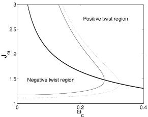
Figure 1: Position of the invariant tori with frequency $(\sqrt{5}-1)/2$ (continuous curve) and $(5+\sqrt{5})/10$ (dashed curve) as a function of $\omega_{c}$ for the integrable Hamiltonian (8) for $e=1$. The strong continuous curve is the location of the twistless region.

The condition of existence of an invariant torus with frequency $\omega$ for $\tilde{H_{0}}$ is $\omega\geq\sqrt{2}\omega_{c}\|V\|$. There are two invariant tori with frequency $\omega$: one located at $J_{\omega}^{-}$ in the negative twist region is a continuation of the torus with frequency $\omega$ in the absence of magnetic field since $\lim_{\omega_{c}\to 0}J_{\omega}^{-}=\omega^{-1/3}$; the other torus located at $J_{\omega}^{+}$ in the positive twist region is created far from the singularity $J=0$ as soon as the field is non-zero. Figure 1 depicts the position of these tori. We notice that as soon as $\omega_{c}\not=0$ there is creation of a set of invariant tori far from $J=0$ in the positive twist region.
If we increase $\omega_{c}$, the position of the positive twist torus decreases whereas the position of the negative twist torus increases. Both tori collide at $\omega_{c}=\omega/\sqrt{2}\|V\|$ to a twistless invariant torus (of the same frequency $\omega$) located at $(\omega/2)^{-1/3}$. The approximate location of this twistless torus as a function of $\omega_{c}$ (for fixed parameter $e$) is plotted in Fig. 1. As one increases $\omega_{c}$, a large portion of the invariant tori with $\omega\in[0,1]$ disappears.

Remark : First Order Delaunay normalization lanc97
Averaging Hamiltonian (6) over $\theta$ gives

$$\langle H\rangle_{\theta}=-\frac{1}{2J^{2}}-L+J^{4}\frac{\omega_{c}^{2}}{8}\|V\|^{2}-\frac{3e}{2}J^{2}F\cos\psi.$$

Using the expansion of $\|V\|^{2}$ to the second order of $e$, $\|V\|^{2}\approx 1+\frac{3e^{2}}{2}$, and the fact that the previous Hamiltonian does not depend on $\theta$ (thus $J$ is constant), the Hamiltonian reduces to

$${\cal K}=-L+\frac{3\omega_{c}^{2}}{16}e^{2}J^{4}-\frac{3}{2}eJ^{2}F\cos\psi,$$

which is the Hamiltonian studied in Ref. lanc97 to find bifurcation of equilibrium points.

II.2 Primary main resonances and Chirikov resonance overlap

The positive and negative twist regions have their own sets of primary resonances given by Hamiltonian (6). The approximate locations of these primary resonances $m$:1, denoted $J_{m}^{\pm}$, are obtained by the condition $m\dot{\theta}+\dot{\psi}\approx 0$. There are two such resonances located approximately at

$$J^{\pm}_{m}=\left(\frac{1\pm\sqrt{1-2m^{2}\omega_{c}^{2}\|V\|^{2}}}{m\omega_{c}^{2}\|V\|^{2}}\right)^{1/3}.$$ (10)

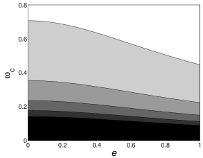
Figure 2: Existence of primary resonances ($m=1,\ldots,5$) in the plane of parameters $e$-$\omega_{c}$. The light gray part is the domain of existence of only $m=1$, and in the black part, all the five first resonances exist.

The resonance located at $J_{m}^{-}$ is the continuation of the resonance in the case $\omega_{c}=0$. The condition of existence of these resonances is $m\sqrt{2}\omega_{c}\|V\|<1$. Similarly to collisions of invariant tori, collisions of periodic orbits occur when increasing $\omega_{c}$. Figure 2 depicts the different domains of existence of real $J_{m}$ for first primary resonances $(m=1,\ldots,5)$ in the plane of parameters $e$-$\omega_{c}$. We notice that the most relevant parameter in this problem is the magnetic field. The variations of the dynamics induced by the eccentricity $e$ are smooth.

Between two consecutive resonances $m$:1 and $m$+1:1 (if they exist), regular and chaotic motions occur for a typical value of the field $F$. In order to estimate the chaos threshold between these resonances, i.e. the value for which there is no longer any rotational invariant torus acting like a barrier in phase space, Chirikov overlap criterion provides an upper bound but usually quite far from realistic values (obtained by numerical integration for instance). For quantitatively accurate thresholds, a modified criterion is applied : the 2/3-rule criterion.

In order to compute the resonance overlap value of the field $F$ between $m$:1 and $m$+1:1 primary resonances, we follow the procedure described in Ref. meer82 . First, we change the frame to a rotating one at the phase velocity of resonance $m$:1. We apply the following canonical change of variables : $(\boldsymbol{A}^{\prime},\boldsymbol{\varphi}^{\prime})=(\tilde{N}^{-1}\boldsymbol{A},N\boldsymbol{\varphi})$ where $\boldsymbol{A}=(J,L)$ and $\boldsymbol{\varphi}=(\theta,\psi)$ and

$$N=\left(\begin{array}[]{cc}m&1\\ 0&1\end{array}\right),$$

and $\tilde{N}$ denotes the transposed matrix of $N$. Hamiltonian (6) is mapped into

$$H= -\frac{1}{2m^{2}J^{\prime 2}}-J^{\prime}-L^{\prime}+\frac{\omega_{c}^{2}}{8}m^{4}J^{\prime 4}\sum_{n,n^{\prime}}V_{n^{\prime}}V_{n^{\prime}-n}\cos[n(\theta^{\prime}-\psi^{\prime})/m]$$

$$+Fm^{2}J^{\prime 2}\sum_{n}V_{n}\cos[(n\theta^{\prime}+(m-n)\psi^{\prime})/m].$$

By averaging over the fast variable $\psi^{\prime}$, the Hamiltonian becomes

$$H=-\frac{1}{2m^{2}J^{\prime 2}}-J^{\prime}+\frac{\omega_{c}^{2}}{8}m^{4}J^{\prime 4}\|V\|^{2}+Fm^{2}V_{m}J^{\prime 2}\cos\theta^{\prime}.$$

The resulting Hamiltonian is integrable and one can compute the width of the resonance $m$:1 following Ref. meer82 . We expand the previous Hamiltonian around $J^{\prime}_{m}=J_{m}/m$ and keep only the quadratic part in $\Delta J^{\prime}=J^{\prime}-J^{\prime}_{m}$ and the constant term in the action $\Delta J^{\prime}$ proportional to $\cos\theta^{\prime}$ :

$$H=-\frac{3m^{2}}{2J_{m}^{4}}\left(1-\frac{1}{2}\omega_{c}^{2}\|V\|^{2}J_{m}^{6}\right)\Delta J^{\prime 2}+FJ_{m}^{2}V_{m}\cos\theta^{\prime}.$$

We rescale energy by a factor $-3m^{2}J_{m}^{-4}(1-\omega_{c}^{2}\|V\|^{2}J_{m}^{6}/2)$ :

$$H=\frac{1}{2}\Delta J^{\prime 2}-\frac{FJ_{m}^{6}V_{m}}{3m^{2}\left(1-\frac{1}{2}\omega_{c}^{2}\|V\|^{2}J_{m}^{6}\right)}\cos\theta^{\prime}.$$

Depending on the positive or negative twist region, this rescaling is positive or negative respectively.

The width of the resonance $m$:1 in the variables $\Delta J=m\Delta J^{\prime}$ is given by :

$$\Delta_{m}=4J_{m}^{3}\sqrt{\frac{FV_{m}(e)}{3}}\left|2-\frac{J_{m}^{3}}{m}\right|^{-1/2},$$

since $\omega_{c}^{2}\|V\|^{2}J_{m}^{6}/2=-1+J_{m}^{3}/m$. The 2/3-rule criterion for the critical threshold for the overlap between resonance $m$:1 and $m$+1:1 is reached when the distance between two neighboring primary resonances is equal (up to a factor $2/3$) to the sum of the half-widths of these resonances :

$$\frac{2}{3}|J_{m+1}-J_{m}|=\frac{1}{2}(\Delta_{m}+\Delta_{m+1}).$$

The critical threshold is given by :

$$F_{m}(e,\omega_{c})=\frac{(J_{m+1}-J_{m})^{2}}{3\left(J_{m}^{3}\sqrt{V_{m}}\left|2-\frac{J_{m}^{3}}{m}\right|^{-1/2}+J_{m+1}^{3}\sqrt{V_{m+1}}\left|2-\frac{J_{m+1}^{3}}{m+1}\right|^{-1/2}\right)^{2}},$$ (11)

where $J_{m}$ stands for either $J_{m}^{+}$ or $J_{m}^{-}$ given by Eq. (10). Therefore we obtain two critical couplings : one in the positive twist region, $F_{m}^{+}(e,\omega_{c})$, and one in the negative twist region, $F_{m}^{-}(e,\omega_{c})$. We notice that for $\omega_{c}=0$, since $J_{m}^{-}=m^{1/3}$, we obtain the formula of Ref. sach97 for the chaos threshold in the CP problem. For $\omega_{c}=1/[\sqrt{2}\|V\|(m+1)]$, the threshold $F_{m}(e,\omega_{c})$ vanishes. This case corresponds to the collision of the resonances $m$+1:1 (the positive and negative twist ones). Therefore, the Chirikov criterion is valid only for $\omega\leq 1/[\sqrt{2}\|V\|(m+1)]$, i.e. when the two primary resonances $m$:1 and $m$+1:1 exist in the system.

We use this criterion in order to study the stability in the different regions of phase space as a function of the magnetic field $\omega_{c}$ (for small values of the field $\omega_{c}$) and the eccentricity of the initial orbit $e$. However, since this criterion is purely empirical, we use another method to validate or refine the results : we use the renormalization method which has proved to be a very powerful and accurate method for determining chaos thresholds in this type of models chan01R ; chan01a ; chan02a ; chan00d . We compare the results given by both methods in the region where the criterion applies and we use the renormalization map to compute chaos thresholds when Eq. (11) does not apply (when one of the main primary resonance $m$:1 has disappeared).

II.3 Renormalization method

The Chirikov resonance overlap criterion gives us a value for the chaos threshold between two neighboring primary resonances. This value aims at approximating the value of the field $F$ for which there is no longer any barrier in phase space, and for which large-scale diffusion of trajectories occur between these resonances. The renormalization method gives a more local and more accurate information. This method computes the threshold of break-up of an invariant torus with a given frequency $\omega$. Then by varying $\omega$, we obtain the global information on the transition to chaos.

II.3.1 Expansion of the Hamiltonian around a torus

In order to apply the renormalization transformation as defined in Refs. chan99c ; chan00a for a given torus with frequency $\omega$, we expand Hamiltonian (2) in Taylor series in the action $J$ around $J=J_{\omega}$.

$$-\frac{1}{2J^{2}}=\sum_{k=0}^{+\infty}(-1)^{k+1}\frac{k+1}{2J_{\omega}^{k+2}}\Delta J^{k},$$

where $\Delta J=J-J_{\omega}$. The meanvalue of the quadratic term in $\Delta J$ of $H_{0}$ is equal to $\frac{3(\omega J_{\omega}^{3}-2)}{2J_{\omega}^{4}}\Delta J^{2}$. We rescale the action variables such that this quadratic term is equal to 1/2, i.e. we replace $H(\Delta J,L,\theta,\psi)$ by $\lambda H(\Delta J/\lambda,L/\lambda,\theta,\psi)$ with $\lambda=3(\omega J_{\omega}^{3}-2)/J_{\omega}^{4}$. We notice that this rescaling can be done except for two cases $J_{\omega}=(\omega/2)^{-1/3}$ which is the twistless case, and for $J_{\omega}=0$ which is the singularity. Therefore, as it is defined in Refs. chan01R ; chan99c ; chan00a , the renormalization cannot be applied in the twistless region.

The Hamiltonian (2) becomes :

$$H_{F}=\omega\Delta J-L+\sum_{k\geq 2}^{+\infty}H_{k,0}\Delta J^{k}+\sum_{k=0}^{4}\sum_{n>0}H_{k,n}\Delta J^{k}\cos n\theta+F\sum_{k=0}^{2}\sum_{n=-\infty}^{+\infty}V_{k,n}\Delta J^{k}\cos(n\theta+\psi),$$ (12)

where

$$H_{2,0}=\frac{1}{2},$$

$$H_{3,0}=\frac{J_{\omega}^{3}(\omega J_{\omega}^{3}+1)}{9(2-\omega J_{\omega}^{3})^{2}},$$

$$H_{4,0}=\frac{J_{\omega}^{6}(11-\omega J_{\omega}^{3})}{108(2-\omega J_{\omega}^{3})^{3}},$$

$$H_{k,0}=\frac{(k+1)J_{\omega}^{3k-6}}{2\cdot 3^{k-1}(2-\omega J_{\omega}^{3})^{k-1}}\qquad\mbox{ for }k\geq 5,$$

$$H_{0,n}=-\frac{3}{4}\omega_{c}^{2}(2-\omega J_{\omega}^{3})\sum_{m=-\infty}^{+\infty}V_{m}V_{m-n},$$

$$H_{1,n}=\omega_{c}^{2}J_{\omega}^{3}\sum_{m=-\infty}^{+\infty}V_{m}V_{m-n},$$

$$H_{2,n}=-\frac{\omega J_{\omega}^{3}-1}{2-\omega J_{\omega}^{3}}\cdot\frac{\sum_{m=-\infty}^{+\infty}V_{m}V_{m-n}}{\|V\|^{2}},$$

$$H_{3,n}=\frac{2J_{\omega}^{3}(\omega J_{\omega}^{3}-1)}{9(2-\omega J_{\omega}^{3})^{2}}\cdot\frac{\sum_{m=-\infty}^{+\infty}V_{m}V_{m-n}}{\|V\|^{2}},$$

$$H_{4,n}=-\frac{J_{\omega}^{6}(\omega J_{\omega}^{3}-1)}{54(2-\omega J_{\omega}^{3})^{3}}\cdot\frac{\sum_{m=-\infty}^{+\infty}V_{m}V_{m-n}}{\|V\|^{2}},$$

$$V_{0,n}=-3V_{n}\frac{2-\omega J_{\omega}^{3}}{J_{\omega}^{2}},$$

$$V_{1,n}=2J_{\omega}V_{n},$$

$$V_{2,n}=-V_{n}\frac{J_{\omega}^{4}}{3(2-\omega J_{\omega}^{3})},$$

for $n\in{\mathbb{Z}}$. The resulting Hamiltonian is of the form :

$$H_{F}(\boldsymbol{A},\boldsymbol{\varphi})=\boldsymbol{\omega}\cdot\boldsymbol{A}+V(\boldsymbol{\Omega}\cdot\boldsymbol{A},\boldsymbol{\varphi}),$$ (13)

where $\boldsymbol{\omega}=(\omega,-1)$ and $\boldsymbol{\Omega}=(1,0)$, and the coordinates are $\boldsymbol{A}=(\Delta J,L)$ and $\boldsymbol{\varphi}=(\theta,\psi)$. For small $F$, the Kolmogorov-Arnold-Moser (KAM) theorem states that if $\omega$ satisfies a Diophantine condition, the invariant torus with frequency $\omega$ will persist. In fact, the picture that emerges from numerical simulations is that if $F$ (in absolute value) is smaller than some critical threshold $F_{c}(\omega)$ then Hamiltonian (2) [or equivalently (12)] has an invariant torus with frequency $\omega$. If $F$ is larger than this critical threshold, the torus is broken. In order to compute numerically the critical function $\omega\mapsto F_{c}(\omega)$, we use the renormalization method described briefly below.

II.3.2 Renormalization method

Without restriction (up to a rescaling of time), we assume that $\omega\in[0,1]$. The renormalization relies upon the continued fraction expansion of the frequency $\omega$ of the torus:

$$\omega=\frac{1}{a_{0}+\frac{1}{a_{1}+\cdots}}\equiv[a_{0},a_{1},\ldots].$$

This transformation will act within a space of Hamiltonians $H$ of the form

$$H(\boldsymbol{A},\boldsymbol{\varphi})=\boldsymbol{\omega}\cdot\boldsymbol{A}+V(\boldsymbol{\Omega}\cdot\boldsymbol{A},\boldsymbol{\varphi}),$$ (14)

where $\boldsymbol{\Omega}=(1,\alpha)$ is a vector not parallel to the frequency vector $\boldsymbol{\omega}=(\omega,-1)$. We assume that Hamiltonian (14) satisfies a non-degeneracy condition : If we expand $V$ into

$$V(\boldsymbol{\Omega}\cdot\boldsymbol{A},\boldsymbol{\varphi})=\sum_{\scriptstyle\boldsymbol{\nu}\in{\mathbb{Z}}^{2}\atop k\geq 0}V^{(k)}_{\boldsymbol{\nu}}(\boldsymbol{\Omega}\cdot\boldsymbol{A})^{k}e^{i\boldsymbol{\nu}\cdot\boldsymbol{\varphi}},$$

we assume that $V_{\boldsymbol{0}}^{(2)}$ is non-zero. This restriction means that we cannot explore the twistless region by the present renormalization transformation.
The transformation contains essentially two parts : a rescaling and an elimination procedure koch99 .

(1) Rescaling : The first part of the transformation is composed by a shift of the resonances, a rescaling of time and a rescaling of the actions. It acts on a Hamiltonian $H$ as $H^{\prime}=H\circ{\mathcal{T}}$ (see Ref. chan00a for details) :

$$H^{\prime}(\boldsymbol{A},\boldsymbol{\varphi})=\lambda\omega^{-1}H\left(-\frac{1}{\lambda}N_{a}\boldsymbol{A},-N_{a}^{-1}\boldsymbol{\varphi}\right),$$ (15)

with

$$\lambda=2\omega^{-1}(a+\alpha)^{2}V^{(2)}_{\boldsymbol{0}},$$ (16)

and

$$N_{a}=\left(\begin{array}[]{cc}a&1\\ 1&0\end{array}\right),$$ (17)

and $a$ is the integer part of $\omega^{-1}$ (the first entry in the continued fraction expansion). This change of coordinates is a generalized (far from identity) canonical transformation and the rescaling $\lambda$ is chosen to ensure a normalization condition (the quadratic term in the actions has a mean value equal to 1/2). For $H$ given by Eq. (14), this expression becomes

$$H^{\prime}(\boldsymbol{A},\boldsymbol{\varphi})=\boldsymbol{\omega}^{\prime}\cdot\boldsymbol{A}+\sum_{\boldsymbol{\nu},k}V^{\prime(k)}_{\boldsymbol{\nu}}(\boldsymbol{\Omega}^{\prime}\cdot\boldsymbol{A})^{k}e^{i\boldsymbol{\nu}\cdot\boldsymbol{\varphi}},$$ (18)

where

$$\boldsymbol{\omega}^{\prime}=(\omega^{\prime},-1)\;\mbox{ with }\omega^{\prime}=\omega^{-1}-a,$$ (19)

$$\boldsymbol{\Omega}^{\prime}=(1,\alpha)\;\mbox{ with }\alpha^{\prime}=1/(a+\alpha),$$ (20)

$$V^{\prime(k)}_{\boldsymbol{\nu}}=r_{k}V_{-N\boldsymbol{\nu}}^{(k)}\;\mbox{ with }r_{k}=(-1)^{k}2^{1-k}\omega^{k-2}(a+\alpha)^{2-k}\left(V^{(2)}_{\boldsymbol{0}}\right)^{1-k}.$$ (21)

We notice that the frequency of the torus is changed according to the Gauss map :

$$\omega\mapsto\omega^{\prime}=\omega^{-1}-\left[\omega^{-1}\right],$$ (22)

where $\left[\omega^{-1}\right]$ denotes the integer part of $\omega^{-1}$. Expressed in terms of the continued fraction expansion, it corresponds to a shift to the left of the entries

$$\omega=[a_{0},a_{1},a_{2},\ldots]\mapsto\omega^{\prime}=[a_{1},a_{2},a_{3},\ldots].$$

(2) Elimination : The second step is a (connected to identity) canonical transformation ${\mathcal{U}}$ that eliminates the non-resonant modes of the perturbation in $H^{\prime}$. Following Ref. chan00a , we consider the set $I^{-}\subset{\mathbb{Z}}^{2}$ of non-resonant modes as the set of integer vectors $\boldsymbol{\nu}=(\nu_{1},\nu_{2})$ such that $|\nu_{2}|>|\nu_{1}|$. The canonical transformation ${\mathcal{U}}$ is such that $H^{\prime\prime}=H^{\prime}\circ{\mathcal{U}}$ does not have any non-resonant mode, i.e. it is defined by the following equation :

$${\mathbb{I}}^{-}(H^{\prime}\circ{\mathcal{U}})=0,$$ (23)

where ${\mathbb{I}}^{-}$ is the projection operator on the non-resonant modes; it acts on a Hamiltonian (14) as :

$${\mathbb{I}}^{-}H=\sum_{\scriptstyle\boldsymbol{\nu}\in I^{-}\atop k\geq 0}V_{\boldsymbol{\nu}}^{(k)}(\boldsymbol{\Omega}\cdot\boldsymbol{A})^{k}e^{i\boldsymbol{\nu}\cdot\boldsymbol{\varphi}}.$$

We solve Eq. (23) by a Newton method following Refs. chan98b ; chan00a .

Thus the renormalization acts on $H$ for a torus with frequency $\omega$ as $H^{\prime\prime}={\mathcal{R}}(H)=H\circ{\mathcal{T}}\circ{\mathcal{U}}$ for a torus with frequency $\omega^{\prime}$.
The critical thresholds are obtained by iterating the renormalization transformation $\mathcal{R}$. The main conjecture of the renormalization approach is that if the torus exists for a given Hamiltonian $H$, the iterates ${\mathcal{R}}^{n}H$ of the renormalization map acting on $H$ converge to some integrable Hamiltonian $H_{0}$. This conjecture is supported by analytical results in the perturbative regime koch99 ; koch99b , and by numerical results chan00d ; chan01a ; chan01R . For a one-parameter family of Hamiltonians $\{H_{F}\}$, the critical amplitude of the perturbation $F_{c}(\omega)$ is determined by the following conditions :

$${\mathcal{R}}^{n}H_{F}\underset{n\to\infty}{\to}H_{0}(\boldsymbol{A})=\boldsymbol{\omega}\cdot\boldsymbol{A}+\frac{1}{2}(\boldsymbol{\Omega}\cdot\boldsymbol{A})^{2}\quad\mbox{ for }F<F_{c}(\omega),$$ (24)

$${\mathcal{R}}^{n}H_{F}\underset{n\to\infty}{\to}\infty\quad\mbox{ for }F>F_{c}(\omega).$$ (25)

The critical threshold $F_{c}(\omega)$ is determined by a bisection procedure.
In order to obtain the value $F_{m}$ of chaos threshold between resonances $m$:1 ans $m$+1:1, we vary $\omega$ between $1/(m+1)$ and $1/m$. The critical threshold is given by $F_{m}=\max_{\omega\in[1/(m+1),1/m]}F_{c}(\omega)$.

III Numerical computation of chaos thresholds

III.1 Chaos thresholds in the negative twist region

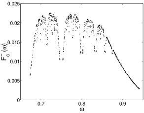
Figure 3: Critical function $F_{c}^{-}(\omega)$ in the negative twist region, obtained by the renormalization method, for $\omega_{c}=0.3$ and for $e=1$.

Figure 3 represents a typical plot of the critical function $\omega\mapsto F_{c}^{-}(\omega)$ in the negative twist region obtained by the renormalization method for $e=1$ and $\omega_{c}=0.3$. This function vanishes at (at least) all rational values of the frequency $\omega$ since all tori with rational frequency are broken as soon as the field is turned on. The condition of existence of a torus with frequency $\omega$ obtained from the integrable case (7) is $\omega>\sqrt{2}\omega_{c}\|V\|$, which is in that case $\omega>0.67$. We expect the tori with frequency belonging to [0,0.67] to be broken by collision with invariant tori in the positive twist region before this value of the field $\omega_{c}$, as it is the case in Hamiltonian (7).

From Fig. 3, we deduce that for $F>F_{c}=0.023$, no invariant tori are left in this region of phase space. The frequency of the last invariant torus is equal to $(\gamma+1)/(2\gamma+1)\approx 0.7236$ where $\gamma=(\sqrt{5}-1)/2$. This value of the frequency of the last invariant torus varies with the parameters $e$ and $\omega_{c}$ (for $\omega_{c}=0$, see Fig. 2 of Ref. chan02a ). The main feature of this frequency is that it remains noble as the parameters $e$ and $\omega_{c}$ are varied, in the sense that the tail of the continued fraction expansion of this frequency is a sequence of 1, or equivalently this frequency expresses like $(a\gamma+b)/(c\gamma+d)$ where $a$, $b$, $c$, $d$ are integers such that $ad-bc=\pm 1$.

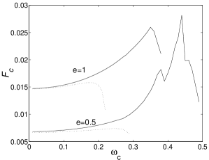
Figure 4: Chaos thresholds $F_{1}^{-}(\omega_{c})$ between resonances 1:1 and 2:1 in the negative twist region, obtained by the 2/3-rule criterion (dashed curves) and by the renormalization method (continuous curves), as a function of $\omega_{c}$, for $e=0.5$ and $e=1$.

We compute chaos thresholds between two successive primary resonances by two methods : the 2/3-rule criterion and the renormalization map. We compute the critical value of the field $F$ for which there is no longer any invariant torus between resonances 1:1 and 2:1, located at $J_{1}^{-}$ and $J_{2}^{-}$ respectively, as a function of the magnetic field $\omega_{c}$ and the parameter $e$ in the negative twist region, i.e. $F_{1}^{-}(e,\omega_{c})=\max_{\omega\in[1/2,1]}F_{c}^{-}(\omega,e,\omega_{c})$. Figure 4 represents two computations : for $e=0.5$ and for $e=1$.

For $\omega_{c}=0$, we obtain the values that have been obtained in Ref. chan02a . The 2/3-rule criterion gives a very good approximation for low values of the field $\omega_{c}$ (typically for $\omega_{c}\in[0,0.15]$). For small $\omega_{c}$, we develop the critical function $F_{1}^{-}(\omega_{c})$ given by Eq. (11). The corrections to $F_{c}^{-}$ due to the magnetic field are of order $\omega_{c}^{2}$ since $J_{n}^{-}=n^{1/3}+O(\omega_{c}^{2}).$

We notice that at some value of $\omega_{c}$, the curves $F_{1}^{-}(e,\omega_{c})$ given by the Chirikov criterion decrease sharply to zero. We have seen that the approximate condition of existence of the resonance $m$:1, derived from the integrable case (8), is $\omega_{c}<1/(\sqrt{2}m\|V\|)$. For $e=1$ and $m=2$, this condition is $\omega_{c}<0.23$ (and for $e=0.5$ this condition becomes $\omega_{c}<0.30$). This means that the criterion derived in Sec. II.2 is inapplicable for $\omega_{c}$ larger than these values ($J_{2}^{-}$ becomes complex). One way of extending this criterion for larger values of $\omega_{c}$ would be to consider the overlap of higher order resonances. From the renormalization map results, we see that after 2:1 resonance disappear, there is an increase of stability which can be explained by the fact that the invariant tori in this region of phase space are no longer deformed by this neighboring resonance. We expect this region to be fully broken before 1:1 disappears (i.e. all the region between 1:1 and 2:1 primary resonances has disappeared), and this happens at $\omega_{c}\approx 0.45$ for $e=1$, and at $\omega_{c}\approx 0.6$ for $e=0.5$. These results are consistent with the sharp decreases of $F_{c}$ found by renormalization on Fig. 4.

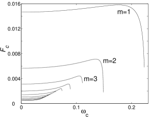
Figure 5: Resonance overlap values of $F_{m}^{-}(\omega_{c})$ between resonances $m$:1 and $m$+1:1 for $m=1,\ldots,10$ in the negative twist region for $e=1$.

Furthermore, we investigate the chaos thresholds for the different primary resonances $m$:1 by the Chirikov criterion. Using Eq. (11), we compute the resonance overlap value of $m$:1 and $m$+1:1 for increasing $m=1,\ldots,10$. For a fixed eccentricity $e=1$, Fig. 5 shows the resonance overlap values as a function of the field $\omega_{c}$

From this figure it emerges that the dynamics in that region is mainly insensitive to the magnetic field for low values of this field. The sharp decreases of the curves $F_{m}^{-}$ are due to the disappearance of one of the primary resonances from which the resonance overlap is computed. At these values and for larger $\omega_{c}$, we expect stability enhancement due to the disappearance of this primary resonance. For $\omega_{c}\geq 1/(\sqrt{2}m\|V\|)$, the critical curve $F_{m}^{-}$ sharply decreases to zero due to the disappearance of all the region between primary resonances $m$:1 and $m$+1:1 into the twistless region. For instance, for $m=3$, the critical curve $F_{3}^{-}(\omega_{c})$ increases slowly with $\omega_{c}$ for $\omega_{c}\in[0,0.11]$, then for $\omega_{c}\in[0.11,0.15]$, we expect stabilization enhancement by the magnetic field, and for $\omega_{c}$ larger than 0.15, the region of phase space between 3:1 and 4:1 resonances disappears into the twistless region and $F_{3}^{-}(\omega_{c})$ vanishes.

The region between resonances of low order ($m$ small) seem to be more stable for $e=1$. However, this feature varies with the parameter $e$ as it has been observed in Ref. chan02a . For $e\in[0,0.8]$ and for $\omega_{c}=0$, the regions near $m$:1 with large $m$ become very stable (and this stabilization is increased by the field for low values of $\omega_{c}$) and the diffusion of the trajectories is very limited. Therefore, the orbits with eccentricity close to one are the easiest to diffuse in a broad range of phase space. In particular, these orbits can ionize more easily than medium eccentricity ones. This feature is expected to hold for small $\omega_{c}$ (typically for $\omega_{c}\leq 0.05$) even if the diffusion is now limited in the negative twist region since we expect the twistless region to be very stable and act as a barrier in phase space cast96 . Figure 6 displays the values of $F_{m}^{-}(e)$ for $e\in[0,1]$, and for two values of $\omega_{c}$ : $\omega_{c}=0.01$ and $\omega_{c}=0.1$.

For $\omega=0.1$, since a large portion of phase space between primary resonances with $m$ large has disappeared into the twistless region, the orbits with medium eccentricity become as easy to ionize as the ones with eccentricity close to one in the remaining part of the negative twist region of phase space. For eccentricities close to one, the critical threshold is dominated by the chaos threshold between resonances 1:1 and 2:1.

In summary, the effect of the magnetic field $\omega_{c}$ is to stabilize the dynamics in the negative twist region by successively breaking up primary resonances. Therefore, between two succesive resonances with $m$ small, the effect of the magnetic field is expected to be smooth in the sense that the critical thresholds are only slightly changed (increased) from the chaos thresholds in the absence of magnetic field up to some critical value of $\omega_{c}$ where collisions of periodic orbits occur. Investigating this region by Chirikov resonance overlap yields values which are qualitatively and quantitatively accurate with respect to the renormalization results for $\omega_{c}\in[0,0.1]$.
For small values of $\omega_{c}$, the qualitative behavior concerning diffusion of trajectories is expected to be the same as the one in the absence of magnetic field even if the diffusion coefficients may be smaller due to the limited region of phase space and the stability enhancement due to the magnetic field. Increasing $\omega_{c}$ makes the orbits with medium eccentricity easier to diffuse in a more and more reduced region of phase space.

III.2 Chaos thresholds in the positive twist region

The classical dynamics in the positive twist region of phase space is essential for the stochastic ionization process since it contains the region where the action $J$ is large, anf for large $\omega_{c}$ this region is the predominant region since the negative twist region shrinks to the singularity $J=0$.

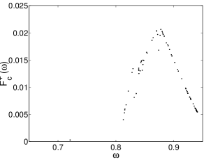
Figure 7: Critical function $F_{c}^{+}(\omega)$ in the positive twist region, obtained by the renormalization method, for $\omega_{c}=0.3$ and for $e=1$.

Figure 7 show a typical critical function $\omega\mapsto F_{c}^{+}(\omega)$ obtained by the renormalization method for $\omega_{c}=0.3$ and for $e=1$. This figure is analogous to Fig. 3.

From Fig. 7, we deduce that for $F>F_{c}=0.021$, no invariant tori are left in this region of phase space. For these values of the parameters $e$ and $\omega_{c}$, the condition of existence of invariant tori $\omega\geq\sqrt{2}\omega_{c}\|V\|$ obtained from the integrable case (7), is $\omega\geq 0.67$. We notice that there is a large chaotic zone for $\omega\in[0.67,0.8]$ (the set of $\omega$ where $F_{c}^{+}(\omega)$ is very small). The diffusion of trajectories throughout the $J$ large region is prevented by the small set of invariant tori with frequency $\omega\in[0.85,0.90]$ for intermediate values of the amplitude of the microwaves $F_{c}\in[0.015,0.02]$. The frequency of the last invariant torus to survive in this region of phase space is approximately equal to 0.87. The frequency of the last invariant torus in the positive twist region fluctuates in a very erratic way as one varies $\omega_{c}$. However we observed that this frequency is always between 0.85 and 0.90 (close to the 1:1 resonance).

The changes induced by the magnetic field are stronger in the positive twist region. We compute the critical thresholds between 1:1 and 2:1 resonances in the positive twist region. Figure 8 represents the results obtained by renormalization and by the 2/3-rule criterion. In this region, the critical thresholds determined by 2/3-rule criterion are well below the ones given by the renormalization for significant values of the field.

Figure 9 represents the critical threshold for the break-up of invariant tori with frequency $\gamma=(\sqrt{5}-1)/2$. In the negative twist region, the golden mean torus is slightly stabilized by the magnetic field. In the positive twist region, the influence of the field is very strong : first, the torus is created then stabilized to high values of the field, then it disappears. This figure shows that in contrast to the negative twist region, the influence of the magnetic field in the positive twist region is very strong. The curve for the positive twist torus appears to have non-smooth variations conversely to the negative twist torus like for instance for $\omega_{c}\approx 0.065$. We notice that for the golden mean tori, there is no break-up by collision since the one located in the positive twist region is broken before the expected collision.

For small values of the field $\omega_{c}$, we expand the threshold given by Chirikov criterion  (11). Since the resonances located at $J_{n}^{+}$ do not exist in the absence of the field $\omega_{c}$, we expect $F_{c}^{+}(m,e,\omega_{c})$ to vanish at $\omega_{c}=0$. The corrections to $F_{c}^{+}$ due to the magnetic field are obtained using the following expansion of $J_{n}^{+}=2^{1/3}n^{-1/3}\|V\|^{-2/3}\omega_{c}^{-2/3}+O(1)$ Thus we have : $F_{m}^{+}(e,\omega_{c})=\alpha_{m}(e)\omega_{c}^{2/3}[1+O(\omega^{2/3})]$, where $\alpha_{m}$ are some constants depending on $e$. This means that the increase of stabilization is very sharp (with infinite slope) for low values of $\omega_{c}$.

Furthermore, using Eq. (11), we compute the 2/3-rule resonance overlap value of $m$:1 and $m$+1:1 resonances for increasing $m=1,\ldots,10$. For a fixed eccentricity $e=1$ , Fig. 10 shows the resonance overlap values as a function of the field $\omega_{c}$ in the positive twist region.

What emerges from this figure is that this region of phase space is strongly stabilized by the magnetic field, and that the curve $m=1$ dominates. However, this feature may vary with the parameter $e$ as it has been observed in Ref. chan02a and in Sec. III.1 for the negative twist region.

These curves are similar to Fig. 6. As a result, increasing the magnetic field makes intermediate eccentricity orbits as easy to ionize (diffusion through a part of phase space where $J$ is large) as the ones with eccentricity close to one. This situation is different from the situation without magnetic field.

The overall effect of the magnetic field in the positive twist region is basically the same as the one in the negative twist region, i.e., it breaks up the primary resonances and fills up the remaining region by very stable invariant tori, preventing the diffusion of trajectories throughout phase space.

IV Conclusion

We have analyzed the classical phase space of the hydrogen atom in crossed magnetic and microwave fields in the high frequency regime. Useful information about the dynamics is provided by the analysis of an integrable part of the Hamiltonian. Accurate information about chaos threshold is obtained by using the renormalization map and the 2/3-rule Chirikov criterion. The global effect of the magnetic field is to stabilize the dynamics and consequently reducing the diffusion of trajectories and the stochastic ionization process.

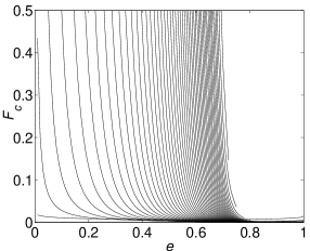
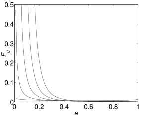
Figure 6: Resonance overlap values of $F_{m}^{-}(e)$ between resonances $m$:1 and $m$+1:1 for $m=1,\ldots$ in the negative twist region for $(a)$ $\omega_{c}=0.01$ and $(b)$ $\omega_{c}=0.1$.

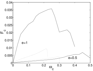
Figure 8: Chaos thresholds $F_{1}^{+}(\omega_{c})$ between resonances 1:1 and 2:1 in the positive twist region, obtained by the 2/3-rule criterion (dashed curves) and by the renormalization method (continuous curves), as a function of $\omega_{c}$. The upper curves are obtained for $e=1$ and the lower ones are for $e=0.5$.

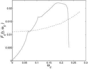
Figure 9: Critical threshold $F_{c}(\gamma,\omega_{c})$ for the break-up of the invariant tori with frequency $\gamma=(\sqrt{5}-1)/2$ for $e=1$ in the positive twist region (continuous curve) and in the negative twist region (dashed curve).

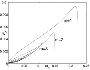
Figure 10: Resonance overlap values of $F_{c}^{+}(\omega_{c})$ between resonances $m$:1 and $m$+1:1 for $m=1,\ldots,10$ in the positive twist region for $e=1$.

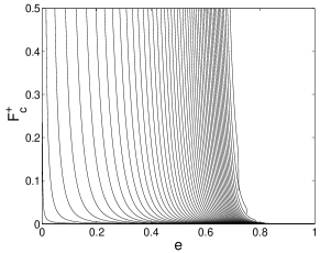
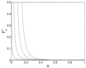
Figure 11: Resonance overlap values of $F_{m}^{+}(e)$ between resonances $m$:1 and $m$+1:1 for $m=1,\ldots$ in the negative twist region for $(a)$ $\omega_{c}=0.01$ and $(b)$ $\omega_{c}=0.1$.

References

- (1) G. Casati, B.V. Chirikov, D.L. Shepelyansky, and I. Guarnieri, Phys. Rep. 154, 77 (1987).
- (2) P.M. Koch and K.A.H. van Leeuwen, Phys. Rep. 255, 289 (1995).
- (3) B.V. Chirikov, Phys. Rep. 52, 263 (1979).
- (4) H. Koch, Erg. Theor. Dyn. Syst. 19, 475 (1999).
- (5) C. Chandre and H.R. Jauslin, to appear in Physics Reports (2002).
- (6) P. Fu, T.J. Scholz, J.M. Hettema, and T.F. Gallagher, Phys. Rev. Lett. 64, 511 (1990).
- (7) M. Nauenberg, Phys. Rev. Lett. 64, 2731 (1990).
- (8) J. Griffiths and D. Farrelly, Phys. Rev. A 45, R2678 (1992).
- (9) D. Wintgen, Z. Phys. D 18, 125 (1991).
- (10) P. Kappertz and M. Nauenberg, Phys. Rev. A 47, 4749 (1993).
- (11) J.E. Howard, Phys. Rev. A 46, 364 (1992).
- (12) K. Sacha and J. Zakrzewski, Phys. Rev. A 55, 568 (1997).
- (13) D. Farrelly and T. Uzer, Phys. Rev. Lett. 74, 1720 (1995).
- (14) A.F. Brunello, T. Uzer, and D. Farrelly, Phys. Rev. A 55, 3730 (1997).
- (15) H. Friedrich, Theoretical Atomic Physics (Springer-Verlag, Berlin, 1991).
- (16) V. Lanchares, M. Inarrea, and J.P. Salas, Phys. Rev. A 56, 1839 (1997).
- (17) B.I. Meerson, E.A. Oks, and P.V. Sasorov, J. Phys. B: At. Mol. Phys. 15, 3599 (1982).
- (18) C. Chandre, Phys. Rev. E 63, 046201 (2001).
- (19) C. Chandre and T. Uzer, to appear in Phys. Rev. E (2002).
- (20) C. Chandre, J. Laskar, G. Benfatto, and H.R. Jauslin, Physica D 154, 159 (2001).
- (21) C. Chandre and H.R. Jauslin, in Mathematical Results in Statistical Mechanics, edited by S. Miracle-Solé, J. Ruiz, and V. Zagrebnov (World Scientific, Singapore, 1999).
- (22) C. Chandre and H.R. Jauslin, Phys. Rev. E 61, 1320 (2000).
- (23) C. Chandre, M. Govin, H.R. Jauslin, and H. Koch, Phys. Rev. E 57, 6612 (1998).
- (24) J.J. Abad and H. Koch, Commun. Math. Phys. 212, 371 (2000).
- (25) D. del Castillo-Negrete, J.M. Greene, and P.J. Morrison, Physica D 91, 1 (1996).