Coupled map gas: structure formation and dynamics of interacting motile elements with internal dynamics

Abstract

A model of interacting motile chaotic elements is proposed. The chaotic elements are distributed in space and interact with each other through interactions depending on their positions and their internal states. As the value of a governing parameter is changed, the model exhibits successive phase changes with novel pattern dynamics, including spatial clustering, fusion and fission of clusters and intermittent diffusion of elements. We explain the manner in which the interplay between internal dynamics and interaction leads to this behavior by employing certain quantities characterizing diffusion, correlation, and the information cascade of synchronization.

,

1 Introduction

High-dimensional dynamical systems with many interacting nonlinear elements have been studied extensively. Here we call such a system “coupled dynamical system”. Among such systems, both those with local coupling and global coupling have been studied at length. For instance, in the study of pattern formation and spatiotemporal chaos, partial differential equations and coupled map lattices (CML) [1, 2] have been employed extensively. In a CML, dynamical elements that are spatially distributed interact with each other through local interactions such as diffusive coupling. The pattern dynamics that arise through the interplay between the internal dynamics of individual elements and their interaction is studied by changing the coupling strength. Globally coupled systems with all-to-all interactions among dynamical elements also represent a typical type of coupled dynamical system [3, 4]. They provide the simplest type of model for complex dynamic networks. Using globally coupled systems, several important concepts in the study of high-dimensional dynamical systems have been developed. Such globally coupled dynamical systems can be considered idealizations of many types of physical, chemical and biological systems.

Coupled dynamical systems cannot always be categorized as either locally coupled or globally coupled. In particular, living systems consist of a huge number of dynamical elements with a variety of scales and with a variety of types of interactions, ranging from local to global. They exhibit interesting collective behavior at the macroscopic level, whose spatiotemporal scales can be much larger than that of individual elements. In such complex systems, even if the properties of each element and the mechanism of its interaction with other elements are well understood, the collective properties of the system are generally much too complicated to be understood without extensive investigation.

In most models of coupled dynamical systems that have been employed to this time, the interaction structure itself is fixed in the sense that the elements with which any given element interacts as well as the nature of the interaction are predetermined. In particular, interacting elements are never decoupled, and non-interacting pairs are never coupled.

In some biological and other types of complex systems, however, the interactions among the dynamical elements can also change in time. For instance, consider a system of motile organisms (e.g. bacteria). Each organism in this system has internal dynamics and interacts with the others. The interaction structure here changes in time according to the motion of the elements. Even within a cell, interactions among molecules change in time. There, enzymatic reactions consist of a finite number of molecules, each of which is a dynamical element having internal states [5]. By sharing a reactive chemical resource, these molecules interact so as to constitute a reaction network. The interactions among the molecules should be time dependent, due to the motion of the molecules. Another example is provided by neural networks, where the coupling between elements changes in time, through the formation and destruction of synaptic connections between neurons.

In order to describe systems of these kinds, we need to construct model coupled dynamical systems whose couplings are dynamic, changing in a manner that depends on the states of individual elements and the interactions between them. In such models, we may find a novel class of collective behavior and self-organization. We thus propose to study the characteristic dynamics of systems in which the interactions between dynamical elements change in time.

There are many possible types of models with internal dynamics, interactions, and motile elements that exhibit interaction structure. Instead of constructing a realistic model specific to some phenomena, we introduce a simple abstract model possessing the above three features. In the present paper, we consider a coupled map whose elements are characterized by spatial positions that change in time. By setting a finite range for the interaction of these motile elements, the existence of an interaction between two given elements will change in time. In this system, we classify several phases with distinct pattern dynamics that depend on the parameters governing the coupling strength, the coupling range, and the internal dynamics. The characteristic dynamics of each phase are elucidated.

This paper is organized as follows. In Section 2, we introduce a simple model of interacting motile dynamical elements constituting a combination and extension of a couple map lattice and a globally coupled map. The model exhibits a variety of phenomena, such as spatial clustering, fusion and fission of the clusters, and intermittent diffusion of the elements. In Section 3, these phenomena are studied for models in one- and two-dimensional space. The global phase diagram is presented in Section 4. Spatial clustering is one of the characteristic dynamical phenomena in the present system. In Section 5, we study this clustering in detail for the case in which the clusters that form are not completely isolated in space but rather interact with each other. Then, in Section 6, we study the case in which each cluster is completely isolated after formation. In Section 7, we study the case in which clusters form structures in space with a scale larger than that of a single cluster. These structures are maintained by the interplay between the internal dynamics of elements and the interactions among elements. The dynamics of the formation of these structures are studied. The paper is concluded in Section 8 with the summary and discussion.

2 Couple map gas as a simple model of interacting motile dynamical elements

To this time, two types of coupled dynamical systems have been investigated, one with local coupling and the other global coupling. Such systems consist of elements with internal dynamics and interactions among them. In the former case, the interactions among elements are restricted locally in space, as in the case of reaction-diffusion equations and coupled map lattices (CML). In particular CMLs with local chaotic dynamics and nearest neighbor interactions have been extensively studied as models of spatiotemporal chaos. The simplest CML model of this kinds is given by

$$x_{n+1}(i)=(1-\varepsilon)f(x_{n}(i))+\frac{\varepsilon}{2}\biggl{(}f(x_{n}(i+1))+f(x_{n}(i-1))\biggr{)},$$ (1)

where $n$ is a discrete time step, $i$ is the site index, and $f(x)=1-ax^{2}$. In the globally coupled case, each element interacts with all other elements. The simplest such model is a globally coupled map (GCM), given by

$$x_{n+1}(i)=(1-\varepsilon)f(x_{n}(i))+{\varepsilon\over N}\sum_{j=1}^{N}f(x_{n}(j)),$$ (2)

where $n$ is a discrete time step, $i$ is the element index, and $N$ is the total number of elements. This model can be regarded as a mean-field version of a CML, or as an infinite dimensional CML. GCMs have also been studied as the simplest models of complex dynamical networks.

In most studies of coupled systems carried out to this time, elements with internal (oscillatory) dynamics are fixed in space, and the structure of the connections between elements is fixed in time; i.e., two elements that are coupled initially are always coupled. The coupling strengths between elements are also constant in most previously studied models, although time dependent coupling strengths have been introduced in some models [6, 7, 8], with connection topologies fixed.

In the present paper, we study a system in which the connections between elements are time dependent in accordance with the motivation expressed in Section 1. For this purpose, we consider the introduction of “motile” elements into CML and GCM models as a natural extension of these systems. Two such elements interact when they are located within a given range in space, and thus the structure of the couplings between elements changes in time due to the motion of the elements. Because the position of elements changes in time, two elements coupled at some time can be decoupled at some other time.

Here, we are interested in general aspects of coupled dynamical systems of motile elements, and for this reason we wish to consider as simple a model as possible. We impose the following conditions on this model:

1. Each element has time-dependent internal state and spatial position.

2. Each element is active in the sense that, even in isolation, its internal state exhibits oscillatory (chaotic) dynamics.

3. The dynamics of the internal state of a given element are affected by local interactions between this and other elements.

4. The elements move through the influence of the force produced by the local interaction, which depends on the internal states of the interacting pair.

In order to construct a model satisfying the above conditions, we stipulate that each element has an internal state represented by a scalar value and is characterized by a time-dependent position in real space. For the dynamics of local internal state, a one-dimensional map that can exhibit chaotic oscillation is employed. The dynamics of the internal state of a given element are influenced by other elements within a distance ${R}$ from this element. This part of the model is basically given in the form of coupled maps. Furthermore, there is a force between elements within the same range, which depends on the internal states of the pair of interacting elements. The motion of the elements in space is governed by these forces. We call the class of models defined in this manner “coupled map gases (CMGs)”.

A simple example of a CMG is given by

$$\begin{array}[]{lll}x_{n+1}(i)&=&\displaystyle(1-\varepsilon)f(x_{n}(i))+\displaystyle{\varepsilon\over N_{n}(i)}\sum_{j\in{\mathcal{N}}(i)}f(x_{n}(j)),\\ \vec{r}_{n+1}(i)&=&\vec{r}_{n}(i)+{\displaystyle\sum_{j\in{\mathcal{N}}(i)}}\frac{\vec{r}_{n}(j)-\vec{r}_{n}(i)}{|\vec{r}_{n}(j)-\vec{r}_{n}(i)|}\mathcal{F}(x_{n+1}(i),x_{n+1}(j)),\end{array}$$ (3)

where $x_{n}(i)$ is the internal state of the $i$-th element at time step $n$, and $\vec{r}_{n}(i)$ is its position in $d$-dimensional space. As the map governing the internal dynamics, we adopt the logistic map $f(x)=1-ax^{2}$, because CMLs and GCMs employing this map have been extensively studied as prototype models of spatiotemporal chaos and network dynamics. In the above equations, $|\vec{r}(j)-\vec{r}(i)|$ is the distance between the $i$-th and $j$-th elements, the set of elements interacting with the $i$-th element is denoted by ${\mathcal{N}}(i)=\{j:|\vec{r}_{n}(j)-\vec{r}_{n}(i)|\leq{R}\}$, and the number of elements in ${\mathcal{N}}(i)$ is denoted by $N_{n}(i)$. Here, $\mathcal{F}(x_{n+1}(i),x_{n+1}(j))$ is a “force”, which depends on the internal states $x$ of the $i$-th and $j$-th elements. In the present paper, we adopt $\mathcal{F}(x(i),x(j))=F\cdot x(i)\cdot x(j)$ as the form of the force, using a fixed parameter $F$. The elements, whose number is fixed at $N$, are located within the fixed spatial domain $[0,L]^{d}$, for which we use periodic boundary conditions.

There are four basic control parameters in our model, $a$, $\varepsilon$, $N(\frac{R}{L})^{d}$ and $\frac{F}{R}$. The role of each control parameter is as follows: $a$ determines the nonlinearity of the local dynamics, $\varepsilon$ is the coupling strength between elements, $N(\frac{R}{L})^{d}$ is the density of elements within the interaction range, and $\frac{F}{R}$ is the effective motility of the elements. Throughout this paper, we fix $\frac{N{R}}{L}\sim 10$, and $\frac{F}{R}\sim 0.01$. The effective motility is chosen to be relatively small so that the motion of each element in space is rather smooth.

Note that the elements in the present model are “active” in the sense that, even in isolation, their internal dynamics can consist of periodic or chaotic oscillation. This strongly contrasts with the situation in recently studied models of the collective motion of flocks [9, 10] and ants [11, 12], in which passive elements are employed.

In the present CMG, the motion in real space is “overdamped”, i.e., in the equation describing this motion, the force term is essentially equated with the velocity, without an acceleration term included. It is rather straightforward to introduce a momentum variable for each element and with it include an acceleration term in the equation of motion. Indeed we have carried out several simulations, with such equations. However, we have found that as long as there is friction force, the important results are unchanged. For this reason, we consider only the overdamped case here.

The choice of the force in Eq.(3) is rather arbitrary. We have imposed the condition that the force between two elements is attractive or repulsive, depending on the signs of the internal states of the interacting elements. With this stipulation, the results we obtained seem to be rather universal for any choice of $\mathcal{F}(x(i),x(j))$. As an alternative type of force, we have also studied the case $\mathcal{F}(x(i),x(j))=\cos[2\pi(x(i)-x(j))]$, and we found that the qualitative features are the same.

When the parameter $F$ is positive, two elements interact attractively if the signs of their internal states are the same, and repulsively if they are opposite. Since the variable $x(i)$ oscillates within the range $[-1,1]$, the sign of the force is correlated with the degree of synchronization of the interacting elements’ oscillations. It should be noted, however, that interaction between two arbitrary elements is attractive on the average if $F$ is positive, because the average of $x$ for a single logistic map (and in the present CMG) is positive for $a<2.0$.

As a type of coupled map system, CMG is a natural extension of a CML in which the condition of the confinement of an element to a single lattice point is removed. If the elements are spontaneously located at positions separated by a distance about $R$, the dynamics of their internal states are those of a CML. On the other hand, for a set of elements located within a distance $R$and separated from other elements, the dynamics of their internal states are those of a GCM. Thus the CMG spontaneously chooses the coupling structure of their internal states ranging from those of a CML to those of a GCM.

In the case of CML or GCM, the variable $x(i)$ of each element can be regarded as a field variable. In the present CMG, in which elements move in space, internal states cannot be regarded as field variables on fixed space. The motion of elements in space can be regarded as dynamics external to the dynamics of the internal state of each element. We are concerned with the “interplay” between such external dynamics and the internal dynamics.

It is also interesting to consider our model from a different viewpoint. Our model (in the 1-dimensional case) can be rewritten as

$$r_{n+1}(i)=r_{n}(i)+f\cdot x_{n+1}(i)\Bigl{(}\sum_{j\in{\mathcal{N}}_{l}(i)}x_{n+1}(j)-\sum_{j\in{\mathcal{N}}_{r}(i)}x_{n+1}(j)\Bigr{)}$$ (4)

where ${\mathcal{N}}_{l}(i)=\left\{j\,;\,j\in{\mathcal{N}}(i),r(j)<r(i)\right\}$ and ${\mathcal{N}}_{r}(i)=\left\{j\,;\,j\in{\mathcal{N}}(i),r(j)>r(i)\right\}$. In this form, the second term on the right hand side is regarded as the gradient of the field at the position $r(i)$, which is determined by the internal state variables $x(i)$ of the elements located within a distance $R$ of $r(i)$. Particles move in this chaotic field, which they themselves form. This interpretation of our model is possible for any spatial dimension.

3 Characteristic phenomena observed in a coupled map gas

Figure 1: Trajectories of elements in the presently constructed CMG in the 1-dimensional case. The temporal evolution of the positions $r(i)$ plotted in time, given by the vertical axis. The trajectory of each element is plotted by drawing a line between successive positions at each step over 250 time steps, after transient behavior has died away. The interval denoted by “R” at the top indicates the coupling range ${R}$.
(a) Fluid phase with $a=1.8$, $\varepsilon=0.12$, $N=100$, ${R}=10.$, $F=0.1$, $L=100$,
(b) Fluid phase with $a=1.8$, $\varepsilon=0.2$, $N=100$, ${R}=10.$, $F=0.1$, $L=100$,
(c) Fluid phase with $a=1.8$, $\varepsilon=0.2$, $N=50$, ${R}=5.$, $F=0.5$, $L=50$,
(d) Intermittent phase with $a=1.8$, $\varepsilon=0.15$, $N=100$, ${R}=10.$, $F=0.1$, $L=100$,
(e) Desynchronized phase with $a=1.8$, $\varepsilon=0.05$, $N=50$, ${R}=5.$, $F=0.1$, $L=50$,
(f) Coherent phase with $a=1.8$, $\varepsilon=0.4$, $N=50$, ${R}=5.$, $F=0.1$, $L=50$.

Figure 2: An example of the evolution of the present CMG in a 2-dimensional space. Time increases from left to right and top to bottom. Each circle represents the position $\vec{r}(i)$ of one element. The internal state of each element is represented by the color of its circle. The snapshots displayed here are separated by four time steps where the first snapshot (at $n=1$) corresponds to the time at which a cluster was formed, beginning from random initial conditions. Periodic boundary conditions are adopted. Here, $a=1.8,\varepsilon=0.3,N=200,{R}=15.0,F=0.2,L=50.0.$

Figure 3: A depiction of the evolution of the present CMG in a 2- dimensional space, for the case that the value of $F$ is negative. The positions of elements at every two time steps are superimposed over 10 time steps; i.e., 5 snapshots are superimposed. The color indicates the internal state of each element –red when the internal state is a positive value and green when it is a negative value. Here, $a=1.8,\varepsilon=0.2,N=200,R=5.0,F=-0.25,L=30.0$

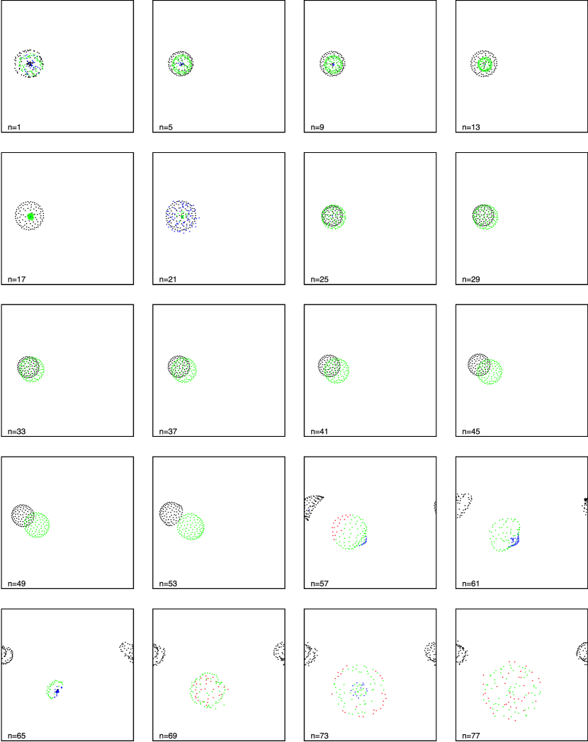
In this section, we give a rough survey of the phenomena observed in the present model, leaving detailed analysis to later sections. Spatiotemporal diagrams of the 1-dimensional system are given in Figure 1, where the trajectories of the elements in real space are plotted by drawing lines between the successive positions of the elements.

To describe the dynamics, it is useful to introduce the notion of a “cluster” in space. Here, a “cluster” is defined as a set of elements that are located in close proximity in such a manner that, as a whole, they are distinguishable from the other elements. With regard to the dynamics of clusters, we note the following three distinct types of behavior:

1. Elements gather to form a cluster whose members are not fixed; i.e., elements enter and leave the cluster over time. Such clusters often split into two, and two clusters often merge into one. This formation and division of clusters occurs repeatedly in time, as shown in Figures 1(a), (b) and (c).

2. Elements form clusters that remain separated by distances approximately equal to ${R}$ from their neighboring clusters. Accordingly elements in each cluster can interact with those in neighboring clusters. In this case, neighboring clusters exchange elements intermittently as shown in Figure 1(d).

3. Clusters are all separated by distances larger than ${R}$. Hence, there are no interactions between elements in different clusters. In this case, the members of each cluster are fixed. Here, the size of each cluster is smaller than ${R}$, so that the dynamics within each cluster are described by a single GCM, as shown in Figures 1(e) and (f).

This classification of the spatiotemporal dynamics displayed by our model is also valid in the 2-dimensional case. Examples of successive instantaneous patterns in the 2-dimensional case are shown in Figure 2. In a 2-dimensional system, there appears a variety of cluster shapes, in addition to those described above. In this situation described by Figure 2, elements start to gather to form a circular cluster. Then, the cluster divides into two new circular clusters. Note that the time evolution begins from random initial conditions. The figure displays only patterns appearing after transient behavior has died away, and after the cluster has first formed. The formation and division of circular clusters seen here is generally observed in the 2-dimensional system.

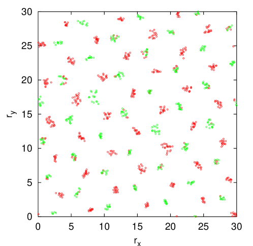
Another example of the 2-dimensional case is depicted in Figure 3. In this example, the value of $F$ is negative. Nevertheless, a lattice structure of clusters is formed. Within a cluster, the forces between elements are repulsive, while the forces between elements of neighboring clusters are attractive. As far as we have studied, the formation of clusters is generic in this class of systems, not restricted to the present CMG.

Although the pattern formation in the 2-dimensional case is interesting, the behavior we have found for the 2-dimensional system to this time can conceptually be understood from the results of the 1-dimensional case. For this reason, we focus on the 1-dimensional case in the remainder of the paper.

4 Global phase diagram

Figure 4: Four typical evolutions of the mean square deviation (MSD) $\langle\delta r^{2}_{t}\rangle=\left\langle\frac{1}{N}\sum_{i=1}^{N}\left(r_{t+t_{0}}(i)-r_{t_{0}}(i)\right)^{2}\right\rangle$ of the positions of the elements, where the average is computed over $10^{5}$ steps, after discarding the initial $10^{4}$ steps and over the number of samples indicated in each plot. Here, $a=1.8$, $N=100$, ${R}=10.0$, $L=100.0$, and $F=0.1$. The four types of behavior seen here correspond to four phases: (a) the coherent phase, (b) the fluid phase, (c) the intermittent phase, and (d) the desynchronized phase.

In this section we characterize the behavior discussed in Section 3 by introducing some statistical measures, and also present the phase diagram of our model. As the measures, we introduce the following three quantifiers, corresponding to the motion in real space, the dynamics of the interaction structure, and the coherence of the oscillatory internal dynamics of the elements.

1. Diffusion of elements: In the simulations we carried out, elements can either move throughout the space or be localized in space, depending on the value of the parameters. In the former case, diffusive, rather than ballistic, motion is observed. Therefore it is useful to introduce a quantity to measure the diffusion of elements. For this purpose we first define the mean square displacement (MSD) of the positions of elements as

   $$\langle\delta r^{2}_{t}\rangle=\left\langle\frac{1}{N}\sum_{i=1}^{N}\left(r_{t+t_{0}}(i)-r_{t_{0}}(i)\right)^{2}\right\rangle,$$ (5)

   where $\left\langle\cdot\right\rangle$ denotes the average over an ensemble of samples. When the MSD increases linearly with $t$, it is possible to define the diffusion coefficient of the elements, characterizing their diffusion in real space, as

   $$D=\lim_{t\rightarrow\infty}\frac{1}{t}\langle\delta r^{2}_{t}\rangle.$$ (6)

2. Change of coupling: Due to the motion of the elements, a pair of elements coupled at one time step can be decoupled at the next time step. The frequency that this change in coupling takes place is a good measure for classifying phases with regard to the fluidity of the interaction. As this measure, we numerically study the conditional probability that a pair of coupled elements remains coupled at the next step (denoted by $P_{CC}$) and the conditional probability that a pair of decoupled elements remains decoupled at the next step (denoted by $P_{DD}$). In the present model, these probabilities are given by

   $$P_{CC}={\mathcal{P}}\Bigl{(}|r_{n}(i)-r_{n}(j)|\leq{R}\,\,\Bigl{|}\,\,|r_{n-1}(i)-r_{n-1}(j)|\leq{R}\Bigr{)}$$ (7)

   $$P_{DD}={\mathcal{P}}\Bigl{(}|r_{n}(i)-r_{n}(j)|>{R}\,\,\Bigl{|}\,\,|r_{n-1}(i)-r_{n-1}(j)|>{R}\Bigr{)}$$ (8)

   for arbitrary $i$ and $j$, where ${\mathcal{P}}({\mathsf{A}|\mathsf{B}})$ is the conditional probability that $\mathsf{A}$ happens given that $\mathsf{B}$ happens. Obviously, the probabilities of the change from coupled to decoupled  ($P_{CD}$) and vice versa ($P_{DC}$) are given by$P_{CD}=1-P_{CC}$ and $P_{DC}=1-P_{DD}$. If there are no coupling changes, $P_{CC}$ and $P_{DD}$ are unity. When there are frequent changes, $P_{CC}$ and $P_{DD}$ take small values.

3. Coherence among the dynamics of internal states: In globally coupled maps, (chaotic) oscillations of all elements are synchronized in the strong coupling regime. Similarly, in the present model, the internal states of elements located within the interaction range ${R}$ can be synchronized when tightly coupled. When the coupling of these elements changes, such synchronization is partially or completely destroyed. Also, weak coherence can be sustained over all elements, even when they are separated by distance greater ${R}$. Therefore, to characterize the system, it is useful to introduce a measure of the degree of coherence.

Figure 5: Diffusion coefficient as a function of $\varepsilon$. $\langle\delta r^{2}_{t}\rangle/t$ is plotted for $t=10000$, from 100 samples. Here, $a=1.8$, $N=100$, ${R}=10$, $L=100$, $F=0.1$.

Four typical types of evolution of the MSD with time are plotted in Figure 4. The diffusion coefficient of the elements given in Eq.(6) calculated from the MSD is plotted as a function of the coupling strength $\varepsilon$ in Figure 5, with $a=1.8$ fixed. From Figure 5, it can be seen that there are three regimes in which the diffusion coefficient is very small. These three regimes are separated by regimes with larger values of the diffusion coefficient. Since the diffusion coefficient plotted in Figure 5 is obtained from the MSD over a finite time ($10^{5}$ steps), it is not possible to conclude that the diffusion coefficient in these three regimes is zero, but we can reach a somewhat certain conclusion by investigating whether the MSD increases with time or eventually stops increasing. Examples of the time evolution of the MSD are displayed in Figure 4.

From the results given in Figures 4 and 5, the following three types of regimes are distinguished.

1. Strong diffusion: There are two such regimes ($0.1\lesssim\varepsilon\lesssim 0.13$ and $0.2\lesssim\varepsilon\lesssim 0.24$ in Figure 5), in which the time evolution of the MSD is clearly proportional to $t$ and the diffusion constant is large.

2. Weak diffusion: In the regime with intermediate coupling strength  ($\varepsilon\approx 0.17$) among the three regimes with small diffusion coefficient, the MSD increases almost linearly with time. Here, the motion of the elements exhibits a diffusive behavior, whose diffusion constant is distinctly smaller than that in the regimes with strong diffusion.

3. No diffusion: For the other two regimes with small values of the diffusion coefficient in Figure 5, i.e., for $\varepsilon\gtrsim 0.25$ and $\varepsilon\lesssim 0.1$, the MSD eventually stops increasing in time. In this case, the elements are localized in space.

Figure 6: The probabilities $P_{CC}$ and $P_{DD}$ defined in the text as functions of $\varepsilon$. They were computed using $10^{4}$ time steps, after transients. The parameter values here are the same as in Figure 5.

Using the above classification based on the diffusion behavior, we can classify the types of cluster dynamics discussed in the last section. These three types of cluster dynamics are characterized as follows.

1. The strong diffusion regimes (a) correspond to case 1 in the last section (see Figures 1(a), (b) and (c)), where the formation and division of clusters continues indefinitely.

2. The weak diffusion regime (b) corresponds to case 2 of the last section (see Figure 1(d)), where clusters form a lattice, and elements are exchanged intermittently between clusters.

3. The no diffusion regime (c) corresponds to case 3 of the last section (see Figures 1(f) and (e)) where each element is localized in a cluster, and each cluster is isolated from the other clusters.

The probabilities $P_{CC}$ and $P_{DD}$ for the changes of couplings are plotted in Figure 6 as a functions of the coupling strength. (There, all other parameters are fixed with the same values as in Figures 4 and 5.) For $\varepsilon\lesssim 0.1$ and $\varepsilon\gtrsim 0.25$, $P_{CC}=P_{DD}=1$, since in these regimes the coupling never changes in time. In the intermediate coupling regime, with a small diffusion coefficient, the probabilities are much smaller than 1. This indicates that changes of couplings take place frequently, even though the diffusion is much slower.

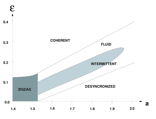
With respect to the three types of quantities discussed above, the MSD, the probabilities $P_{CD}$ and $P_{DC}$ and the coherence, we have succeeded in classifying the behavior of the present CMG into the following five phases: 1) coherent phase, 2) fluid phase, 3) intermittent phase, 4) desynchronized phase, 5) checkered phase. The phase diagram is given in Figure 7 and the characteristic features of each phase are summarized in Table 1

Figure 7: The global phase diagram of CMG.

We now describe these phases in detail.

Coherent phase:

When the coupling strength is sufficiently large, elements do not diffuse in space, as shown in Figures 4(a) and 5. In this case, the coupling among elements does not change, as shown in Figure 6. The spatiotemporal diagram corresponding to this phase is given by Figure 1(f). Here, it is seen that elements split into disconnected clusters separated by distances larger than the interaction range ${R}$. Therefore, there are no interactions between clusters. Within each cluster, all elements are coupled to each other. Since all clusters are completely decoupled, the dynamics of the elements in each cluster are reduced to those of a globally coupled map whose total number of elements is the number of elements in the cluster. Within each cluster, the internal oscillations of elements are synchronized. Thus the coherence in this phase is that of the complete synchronization case of the GCM.

Fluid phase:

When the coupling strength is sufficiently smaller, elements diffuse rapidly, as shown in Figures 4(b) and 5. In this case, the couplings among elements change frequently, as shown in Figure 6. In this phase, the formation and division of clusters is repeated indefinitely, as shown in the spatiotemporal diagram given by Figures 1(a), (b) and (c). In this phase, the cluster structure is dynamic, and its evolution is determined by the interplay between the internal dynamics of interacting elements and the motion of the elements. We discuss these dynamics in more detail in Section 5.

Intermittent phase:

In the midst of the fluid phase, there exists a region in which the diffusion coefficient is distinctively small but non-zero, as shown in Figures 4(c) and 5. Even though the diffusion here is quite weak, the coupling among elements change quite frequently as shown in Figure 6. In this case, the clusters form a lattice structure depicted in Figure 1(d), which is almost static with only the intermittent exchanges of elements.

Desynchronized phase:

When the coupling strength is even smaller, beyond a certain value, the elements no longer diffuse, as shown in Figures 4(c) and 5. In this case, the coupling among elements also does not change, as shown in Figure 6. Here, clusters are separated by distances greater than ${R}$ (as in Figure 1(e)) and therefore do not interact, while within each cluster all elements interact with each other, and the oscillations of elements are desynchronized. Because all clusters are completely separated, the internal dynamics here are those of the desynchronized state of the GCM.

Checkered phase:

There exists another phase in a region with a smaller value of the nonlinearity parameter $a$, in which the couplings among elements change frequently, but elements do not diffuse in space. In this case, two neighboring clusters are separated by a distance approximately equal to ${R}$. Some elements between neighboring clusters interact with each other at some time steps, but they can be separated by distances greater than ${R}$ at some other times. This is the reason that here the probabilities $P_{CC}$ and $P_{DD}$ are smaller than 1. Within each cluster, oscillations are strongly correlated, while oscillations of neighboring cluster are out of phase. In this phase, elements exhibit period-2 band oscillations. Denoting the state of $x(i)$ only by its sign, all elements in a given cluster oscillate as $+\rightarrow-\rightarrow+\rightarrow-\rightarrow+\rightarrow\cdots$, while those in a neighboring cluster oscillate perfectly out of phase as $-\rightarrow+\rightarrow-\rightarrow+\rightarrow\cdots$. Thus the states $x$, when represented in this way, form a checkered spatial pattern among cluster.

	Diffusion	Change of Coupling	Coherence among internal dynamics
Coherent Phase	$\times$	$\times$	$\bigcirc$
Fluid Phase	$\bigcirc$	$\bigcirc$	$\times$
Intermittent Phase	$\bigcirc$(weak)	$\bigcirc$(frequent)	$\bigcirc$(Zigzag)
Desynchronized Phase	$\times$	$\times$	$\times$(Desynchronized)
Checkered Phase	$\times$	$\bigcirc$	$\bigcirc$(Checkered)

Table 1: The characteristics of each phase. (See text for details.)

5 Formation and collapse of clusters in the fluid phase

In a coupled dynamical system, the dynamics of elements often become synchronized so that they come to form groups in phase space. Such groups are often also referred to as “clusters” [3, 13]. In the present case, such synchronization of oscillations influences the formation and collapse of clusters in real space. Conversely, the motion of elements in real space influences the internal dynamics of elements. As a result, formation, fusion and fission of the clusters occur repeatedly in the fluid phase. Studying the interrelation between the internal dynamics and the motion in real space, we have found that the process of cluster formation, fission and fusion in space can be described as follows.

step 1.

The interactions among elements tend to synchronize the internal states of elements. However, chaotic nature of the internal dynamics tends to destroy this synchronization. When synchronization dominates, forces between elements on the average become attractive, and clusters are formed.

step 2.

Within each cluster, the dynamics are of a GCM type (to the extent that the influence of neighboring clusters can be ignored). A number of synchronized groups are formed among the elements in a cluster.

step 3.

In some of such groups the sign of the internal states evolve as $+\rightarrow-\rightarrow+\rightarrow-\rightarrow\cdots$, while that of in other groups evolve as $-\rightarrow+\rightarrow-\rightarrow+\rightarrow\cdots$. Then, the force between two elements from such two types of groups is repulsive, while the force between the elements within the same type of group is attractive.

step 4.

Due to the repulsive forces between groups, the cluster divides into two new clusters, if the cumulative force is sufficiently strong. This repulsion continues until the distance between the two new clusters is larger than ${R}$. Consequently, the two new clusters come to be located at a distance of about ${R}$.

step 5.

When the distance between the two new clusters becomes larger than ${R}$, they no longer interact. Initially, almost all elements within one of these clusters (i.e., elements within the range ${R}$) are nearly synchronized, but this state is unstable, because synchronized chaos in the GCM is unstable in this parameter region. Thus the process returns to step 2. Thus each cluster has the potentiality of repeated division.

step 6.

If a cluster interacts with other clusters, depending on the internal dynamics of these clusters, these clusters can fuse together. Then, the evolution of this newly merged cluster returns to step 2.

In this way, the fusion and fission processes of clusters continues indefinitely.

Figure 8: The information creation per bit $I^{(m)}_{n}$, the $m$-bit entropy $s^{(m)}_{n}$ for $m=10$, the conditional probability $P_{CD}+P_{DC}$ and the spatial entropy ${\mathcal{S}}_{n}$ plotted as functions of time for the fluid phase. Here, $a=1.8,\varepsilon=0.2,N=100,{R}=10.,F=0.1,L=100.$

In order to understand the above described process in a more quantifiable manner, we now characterize the behavior of the spatial motion and the internal degrees of freedom quantitatively.

In the fluid phase, one of the most important processes in the internal dynamics is the synchronization. In the synchronization process, the difference between the internal variables of two elements decreases with time. This process can be effectively seen by measuring the information creation per bit $I^{(m)}_{n}$, introduced in Ref.[14], where $n$ is a discreate time step and $m$ is a particular integer value. For this, we partiton the space of the internal state into intervals of a size $2^{-m}$. Then, we define the distribution function $P^{(m)}_{n}(j),\quad(j=0,\cdots,2^{m+1}-1)$ as the fraction of elements whose internal states take values in the interval $[j\times 2^{-m}-1,(j+1)\times 2^{-m}-1]\quad(j=0,\cdots,2^{m+1}-1)$ at time step $n$. Here, we disregard the position of each element. Then, the information creation per bit $I^{(m)}_{n}$ at time step $n$ is defined by

$$I^{(m)}_{n}=s^{(m)}_{n}-s^{(m-1)}_{n},$$ (9)

where $s^{(m)}_{n}$ is the $m$-bit entropy at time step $n$ given by

$$s^{(m)}_{n}=-\sum_{j=0}^{2\times 2^{m}-1}P^{(m)}_{n}(j)\log{P^{(m)}_{n}(j)}.$$ (10)

Since the $m$-bit entropy is a nondecreasing function of $m$, $I^{(m)}$ cannot take a negative value. If two elements are synchronized to a precision of $2^{-\ell+1}$, the value of $s^{(m)}$ increases at $m=\ell$. Therefore $I^{(m)}$ takes a positive value when $m=\ell$, while $I^{(m)}$ equals zero for values of $m$ less than $\ell$. If the two elements are becoming synchronized, the largest value $m=\ell$ at which $s^{(m)}$ increases and $I^{(m)}$ is non-zero increases with time. Thus, the synchronization process can be viewed as the increase of the largest value of $m$ for which $I^{(m)}$ is greater than zero.

At the bottom of Figure 8, $I^{(m)}_{n}$ for $\quad m=2,\cdots,30$ is plotted as a function of time. Several synchronization processes can be seen in this figure, as the increase of the largest value of $m$ for which $I^{(m)}_{n}>0$. In Figure 8, the time evolution of the $m$-bit entropy $s^{(m)}_{n}$ is also plotted for $m=10$. This entropy measures the degree to which elements are synchronized. The synchronization processes can also be identified by the decrease of $s^{(10)}_{n}$, while once synchronization has been established, its breakdown can be identified by the increase of $s^{(10)}_{n}$.

Change in the spatial configuration of elements is characterized by the spatial entropy. First, we partition the entire space into intervals of a given size. Then we define the the fraction of elements in each interval $j$ as ${Q_{n}(j)}$. Here, the width of an interval is chosen to be approximately the same as the effective width of the cluster (see the caption of Figure 9). In our simulations, we chose the value $L/64$. The spatial entropy is computed as

$${\mathcal{S}}_{n}=-\sum_{j=1}Q_{n}(j)\log{Q_{n}(j)}.$$ (11)

 From the time evolution of ${\mathcal{S}}_{n}$ displaying in Figure 8, one can see that ${\mathcal{S}}_{n}$ decreases in the process of cluster formation and increases in the process of cluster collapse.

In Figure 8, ${\mathcal{S}}_{n}$ is plotted as a function of time. As the synchronization proceeds, as is shown by the increase of the largest $m$ for which $I^{(m)}>0$, the decrease of the spatial entropy ${\mathcal{S}}_{n}$ is observed. This indicates cluster formation processes. After the synchronization process becomes completed, the spatial entropy ${\mathcal{S}}_{n}$ stops decreasing. Then, ${\mathcal{S}}_{n}$ begins to increase, indicating that the process of cluster collapse has begun. The collapse of cluster accompanies the breakdown of the synchronization among the internal dynamics of its element. As a result, the $m$-bit entropy $s^{(10)}_{n}$ also begins to increase. In Figure 8, the conditional probability $P_{CD}+P_{DC}$ is plotted as a function of time, indicating the frequency of coupling change (see Section 4). From this, it is seen that the collapse of a cluster leads to an increase in the frequency of coupling change.

In this way, the formation and collapse of clusters take place repeatedly due to the interplay between the internal dynamics and the spatial motion of the elements. Such processes are expected to take place at any point in space. Although $I^{(m)}_{n}$, $s^{(m)}_{n}$, $P_{CD}+P_{DC}$ and ${\mathcal{S}}_{n}$ are computed by treating all elements identically without taking account of spatial structures, we can clearly see the processes of cluster formation and collapse reflected in the behavior of these averaged quantities.

6 Absence of fusion and fission of clusters in the coherent and desynchronized phases

In this section, we study cases in which neither fusion nor fission of clusters takes place once clusters are formed. One such case is in the coherent phase with the coupling strength sufficiently large, and the other is in the desynchronized phase with the coupling strength sufficiently small.

In the case of the coherent phase, elements in a cluster interact with each other strongly, so that the internal dynamics of the elements in the same cluster are highly synchronized. It is the attraction among elements resulting from synchronization that causes a cluster to form. For a system in the synchronized state, beginning from random initial conditions, after transient behavior dies away, clusters are formed and exist isolated in space, with no interaction among them. Hence, the internal dynamics of the elements in any given cluster are those of a GCM in its coherent state. If coherent oscillation of these isolated GCM systems is stable, this stable cluster formation is guaranteed, and the resulting clusters will be separated by a distance greater than ${R}$.

In the case of the desynchronized phase, elements are coupled weakly, so that there is no synchronization, and the coherence among the internal dynamics of elements is weak. Even in such a case, the elements form clusters that are also separated by distances greater than ${R}$, and again there exists no interaction among clusters. In this case, within a cluster, the internal dynamics of the elements are those of the desynchronized state of a GCM. Then, the forces between elements change sign frequently, and the interactions between elements can often be repulsive. Thus the reason that no elements escape from a cluster is not immediately evident.

A possible reason for this fact may be that the sum of forces among the elements gives an attraction towards the center of the cluster, even if each two-body force is repulsive. In order to check if this could be the case, the direction and strength of the force acting on each element was calculated as a function of the distance from the center of mass of the cluster. The strength of the force was calculated as follows. The strength of the force acting on an element is given by the second term on the right hand side of Eq.(3). Then, the position of an element in the cluster is defined by its distance from the center of the cluster. Here, the center of a cluster is defined as the center of mass of the elements that are located within a distance $d$ of a given element at a given time step. Since even elements that directly interact with each other can be members of different clusters, $d$ should be smaller than ${R}$. The strength of the force on an element and its fluctuation as functions of the position can depend on the distance $d$. However, if a well-defined cluster exists, there should be a range of values of $d$ for which the value of the force calculated in this manner does not strongly depend on $d$. We take the value of $d$ within such an interval. The position of the center of a cluster computed in this way, by choosing an arbitrary element, is approximately the same for any chosen element within the cluster.

Figure 9: (a) and (b): The strength of the force acting on an element and its fluctuation as functions of the position of the element in the cluster. In the case of (a), elements stay within the range $[-0.77,0.77]$ with probability $90\%$, and within the range $[-1.22,1.22]$ with probability $95\%$. We can consider the lengths of these intervals are roughly the effective width of the clusters. (c) and (d): The position of an element at one time step as a result of the force experienced at the previous time step as a function of the position. (For the method of calculation, see the text.) The average strength of the force and its fluctuation were computed over $10^{4}$ time steps, after discarding the initial $5000$ steps, and averaged over $100$ samples, starting from random initial conditions. Here, $a=1.8,N=100,{R}=10.0,F=0.1,L=100.0$, (a) $\varepsilon=0.2$, $d=4.0$, (b) $\varepsilon=0.075$, $d=5.0$, (c) $\varepsilon=0.2$, $d=4.0$, (d) $\varepsilon=0.075$, $d=5.0$.

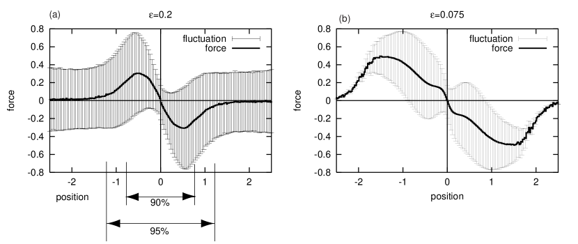
In Figures 9(a) and (b), the strength of the force experienced by an element and its fluctuation are plotted as functions of the position, and in Figure 9(c) and (d), the position of an element at one time step as a result of the force experienced at the previous time step is plotted as a function of the positions. In both the cases of the fluid phase, in (a) and (c), and the desynchronized phase in (b) and (d), elements around the center of the cluster are attracted to the center, on average. However, by taking the fluctuations into account, these two phases are clearly distinguished.

For the fluid phase, the fluctuation (indicated by the error bars in the figure) always crosses over the line $y=x$ in Figure 9(c). It is thus seen that elements can occasionally escape from the cluster. For the desynchronized phase, by contrast, the fluctuation does not cross over the line $y=x$ for positions within a particular range near when attractive force disappears. This indicates that in the desynchronized phase, the elements around the edge of the cluster are with certainly attracted to the center, and therefore elements cannot escape from the cluster. We thus understand that the collective attraction in the desynchronized phase is the source of cluster formation.

7 Structure formation and weak diffusion in the intermittent phase

Figure 10: Power spectrum, $P(k)=\left\langle\frac{1}{N}\sum_{j=1}^{N}x(j)e^{2\pi\mathrm{i}kr(j)}\right\rangle$. The vertical lines in the figure are at intervals of $\frac{1}{2{R}}$. The average is computed over $10^{4}$ time steps, after discarding the initial $10^{4}$ steps and averaged over $10$ samples starting from random initial conditions. Here, $a=1.8,N=400,{R}=10.0,F=0.1,L=400.0$, (a) intermittent phase $\varepsilon=0.15$ (b) fluid phase $\varepsilon=0.2$.

In this section we study the intermittent phase by considering structure formation and intermittent behavior.

In the intermittent phase, after transient behavior has died out, through the repeated fusion and fission of clusters, clusters eventually form a lattice structure with a nearly fixed spacing ${R}$ (see Figure 1(d)). This lattice structure can be clearly characterized by the power spectrum defined as

$$P(k)=\left\langle\frac{1}{N}\sum_{j=1}^{N}x(j)e^{2\pi\mathrm{i}kr(j)}\right\rangle,$$ (12)

in which the internal degrees of freedom are also taken into account. Figure 10 displays typical power spectra for the intermittent phase and the fluid phase. The sharp peaks in Figure 10(a) indicate the formation of lattice structure over a long spatial distance. The first peak is located at the wave number $\frac{1}{2{R}}$ not $\frac{1}{R}$, implying some structure with wavelength $2{R}$. This is because the internal degrees of freedom of the elements in a cluster are approximately in phase, whereas those of the elements of neighboring clusters are of nearly opposite phase. Hence the clusters form a checkered pattern, and the wavelength is ${2R}$. Even in the case of the fluid phase, depicted in Figure 10(b), there is a peak at around the wave number $\frac{1}{2{R}}$. This peak is not as sharp here as it is in the case of the intermittent phase, due to the successive formation and collapse of clusters.

Figure 11: The information creation per bit $I^{(m)}_{n}$, the $m$-bit entropy $s^{(m)}_{n}$ for $m=10$, the conditional probability $P_{CD}+P_{DC}$, and the spatial entropy ${\mathcal{S}}_{n}$ as functions of time for the intermittent phase. Here, $a=1.8,\varepsilon=0.15,N=100,{R}=10.,F=0.1,L=100.$

In the fluid phase, synchronization among elements leads to the formation of clusters, as shown in Section 5, where the synchronization process was characterized by the information creation per bit, $I^{(m)}_{n}$. In the intermittent phase, the internal dynamics of elements within a cluster are roughly in phase. In contrast to the fluid phase, these dynamics do not exhibit any symptoms of synchronization among elements. In Figure 11, $I^{(m)}_{n}$ is plotted as a function of time. No increase of the largest value of $m$ for which $I^{(m)}_{n}>0$ is observed. This indicates that no synchronization process takes place.

If one cluster is isolated from the lattice structure, in phase motion within the cluster cannot be maintained and as a result, the cluster divides into two. Thus, in the intermittent phase, the interactions among clusters are essential for the formation of clusters. As shown in Figure 6, the high activity of interaction between clusters also suggests the importance of interactions.

In spite of the absence of synchronization among elements and the frequent change of the interactions among clusters, the diffusion constant in the intermittent phase is extremely small but not zero, as shown in Figure 5. This indicates that the structure is stable most of the time. Then, we are faced with the question of why this structure is so stable.

Figure 12: (a) The strength of the force acting on an element and its fluctuations as functions of the position of the element in the cluster. (b) The position of an element at one time step as a result of the force experienced at the previous time step as a function of the position. (For the calculation, see the text in Section 6.) The average strength of the force and its fluctuation were computed over $10^{4}$ steps, after discarding the initial $5000$ steps, and averaged over $1000$ samples, starting from random initial conditions. Here, $a=f1.8,\varepsilon=0.15,N=100,{R}=10.0,F=0.1,L=100.0$, and $d=\frac{R}{2}$.

To answer this question, we recall the collective attraction phenomena in a cluster investigated in the previous section. In Section 6, it was seen that in the desynchronized phase, when we plot the direction and the strength of force acting on an element as a function of the position of the elements in the cluster, we find that there is a collective attraction of elements that acts to form a cluster. Hence, in this case, there exists no interaction among clusters and no diffusion of elements. We also calculated the force and its fluctuation in the present case. In Figure 12(a), the average force experienced by an element is plotted as a function of its position, and the position at one time step as a result of the force experienced at the previous time step is plotted in Figure 12(b). As shown, there is an average attractive force exerted an element around the center of the cluster, and there is a region in which the fluctuation of the force is not large enough to change its sign. The position at one time step, as a function of that of at the previous time step does not cross over the diagonal line $y=x$, except the center. This indicates the elements remain in a cluster for a very long time. We should note that in the present case, it is the interactions among the neighboring clusters that causes the structure to be stable. On the other hand, there are some neutral zones, where the force is nearly zero (and the next position is around the $y=x$ line) at positions larger than about 1.0. This leads to the intermittent switch of elements among neighboring clusters.

8 Summary and Discussion

In this paper we have proposed an abstract model, a coupled map gas, in order to study coupled dynamical systems whose couplings change in time in a manner that depends on the states of the system elements and their interactions. For this purpose, we introduced “motility” in space for the elements in our model, which represents a combination and extension of CML and GCM systems. In the present model, active elements with internal dynamics move through space and as determined by their interactions with the other elements. The internal state of each element is determined by these interactions as well as by its own intrinsic dynamics. As a result of their motion in space, the couplings among elements can change in time.

The present model exhibits a variety of phenomena. One of the most characteristic types of behavior of this system is the formation of clusters in space. These clusters are not isolated, but rather interact with each other. As a result of such interactions, clusters exchange elements. The formation and collapse of clusters occur repeatedly. Depending on the parameter values, clusters can form a lattice structure. In such a case, the exchange of elements between clusters is only intermittent.

The above mentioned phenomena were studied here from the viewpoint of the interplay between the internal and external dynamics. As studied in Section 7, the clusters form a stable lattice structure, in which the internal oscillations of the elements in neighboring clusters are out of phase with each other. Thus, there are two kinds of elements, whose internal states have one of the two different phases. However, this formation of lattice structure is not a simple pattern formation of the ordering of two kind of elements, as is indicated by the intermittent diffusion of elements. On the one hand, the internal dynamics of an element depend on its position in the structure. As a result, two kinds of elements with different types of internal dynamics emerge. On the other hand, the existence of two kinds of elements leads to the formation of lattice structure. Some balance between the effects of the dynamics of spatial degrees of freedom and the dynamics of internal degrees of freedom is essential to the formation of stable structure here.

As the coupling strength is increased or the nonlinear parameter of the elements is decreased, there is an increasing tendency toward the synchronization. In this case, elements in a cluster can form synchronized groups with oscillations of different phases. As a result, the lattice structure becomes destabilized, and the formation and collapse of clusters take place repeatedly. Conversely, as the coupling strength is decreased or the nonlinear parameter is increased, the dynamics of each element become too chaotic to allow the formation of groups with correlated phases of oscillation. In this case too, lattice structure is destabilized, and again clusters form and collapse repeatedly.

In this paper we have discussed a novel type of structure formation and dynamics in a system of interacting motile elements with internal dynamics. Often, this structure is not rigid and is flexible, due to the interplay between the internal dynamics and the interactions. Structure formation and collective dynamics of active elements are widely seen in a biological systems as well as in a biological-type physico-chemical systems. The presently studied coupled map gas system may be too simple and abstract to capture all the complexity of such biological systems. Still, due to the universality in the class of systems possessing interaction motile elements of the behavior we have investigated, we expect that the present study will sheds a new light on the understanding of collective dynamics in biological systems.

The authors would like to thank S. Sasa, T. Ikegami, M. Sano and A. Mikhailov for useful discussions. This research was supported by Grants-in-Aid for Scientific Research from the Ministry of Education, Culture, Sports, Science and Technology of Japan (11CE2006). T. S. gratefully acknowledges the support from the Alexander von Humboldt Foundation (Germany).

References

- [1] K. Kaneko, ‘Period-doubling of kink-antikink patterns, quasi-periodicity in antiferro-like structures and spatial intermittency in coupled logistic lattice –toward a prelude to a “field theory of chaos”—’, Progress of Theoretical Physics 72, (19984) 480.
- [2] K. Kaneko, ed., Theory and Applications of Coupled Map Lattices, (Jon Wiley & Sons, New York, 1993).
- [3] K. Kaneko, “Clustering, Coding, Switching, Hierarchical Ordering, and Control in Network of Chaotic Elements”, Physica 41D (1990) 137.
- [4] T. Shibata and K. Kaneko, “Tongue-Like Bifurcation Structures of the Mean-Field Dynamics in a Network of Chaotic Elements”, Physica 124D (1998) 163–186.
- [5] A. Mikhailov and B. Hess, “Microscopic Self-Organization of Enzymic Reactions in Small Volumes”, J. Phys. Chem. 100, (1996) 19059-19065
- [6] K. Kaneko, “Relevance of Clustering to Biological Networks”, Physica 75 D (1994), 55-73
- [7] J. Ito and K. Kaneko, “Self-organized hierarchical structure in a plastic network of chaotic units” Neural Networks 13 (2000) 275-281
- [8] J. Ito and K. Kaneko, “Spontaneous structure formation in a network of chaotic units with variable connection strengths”, Phys. Rev. Lett., 88 (2002) 028701-1
- [9] A. Czirók and T. Vicsek, “Collective behavior of interacting self-propelled particles”, Physica A 281 (2000) 17
- [10] Y. Hayakawa, T. Mizuguchi, M. Sano, N. Shimoyama, and K. Sugawara, “Collective motion in a system of motile elements”, Phys. Rev. Lett. 76 (1996) 3870-3873.
- [11] O. Miramontes, R. V. Sole and B. C. Goodwin, “Collective behavior of random-activated mobile cellular automata”, Physica 63D, (1993) 145–160.
- [12] B. J. Cole, “Is animal behavior chaotic? evidence from the activity of ants”, Proc. R. Soc. Lond. 224B, (1991) 253–259.
- [13] K. Okuda, “Variety and generality of clustering in globally coupled oscillators”, Physica D63, (1993) 424–436; N. Nakagawa,and Y. Kuramoto, “Collective chaos in a population of globally coupled oscillators”, Progress of Theoretical Physics 89, (1993) 313–323.
- [14] K. Kaneko, “Information Cascade with Marginal Stability in Network of Chaotic Elements”, Physica D 77 (1994), 456-472