The clustering instability of inertial particles spatial distribution in turbulent flows
Abstract
A theory of clustering of inertial particles advected by a turbulent velocity field caused by an instability of their spatial distribution is suggested. The reason for the clustering instability is a combined effect of the particles inertia and a finite correlation time of the velocity field. The crucial parameter for the clustering instability is a size of the particles. The critical size is estimated for a strong clustering (with a finite fraction of particles in clusters) associated with the growth of the mean absolute value of the particles number density and for a weak clustering associated with the growth of the second and higher moments. A new concept of compressibility of the turbulent diffusion tensor caused by a finite correlation time of an incompressible velocity field is introduced. In this model of the velocity field, the field of Lagrangian trajectories is not divergence-free. A mechanism of saturation of the clustering instability associated with the particles collisions in the clusters is suggested. Applications of the analyzed effects to the dynamics of droplets in the turbulent atmosphere are discussed. An estimated nonlinear level of the saturation of the droplets number density in clouds exceeds by the orders of magnitude their mean number density. The critical size of cloud droplets required for clusters formation is more than m.
pacs:
47.27.Qb, 05.40.-aI Introduction
Formation and evolution of aerosols and droplets inhomogeneities (clusters) are of fundamental significance in many areas of environmental sciences, physics of the atmosphere and meteorology (e.g., smog and fog formation, rain formation), transport and mixing in industrial turbulent flows (like spray drying, pulverized-coal-fired furnaces, cyclone dust separation, abrasive water-jet cutting) and in turbulent combustion (see, e.g., CST98 ; T77 ; C80 ; S86 ; EKPR97 ; SR98 ; EKRI98 ; VY00 ). The reason is that the direct, hydrodynamic, diffusional and thermal interactions of particles in dense clusters strongly affect the character of the involved phenomena. Thus, e.g., enhanced binary collisions between cloud droplets in dense clusters can cause fast broadening of droplet size spectrum and rain formation (see, e.g., VY00 ). Another example is combustion of pulverized coal or sprays whereby reaction rate of a single particle or a droplet differs considerably from a reaction rate of a coal particle or a droplet in a cluster (see, e.g., AR92 ; ARD94 ).
Analysis of experimental data shows that spatial distributions of droplets in clouds are strongly inhomogeneous (see, e.g., PB89 ; KM93 ; B99 ; KS01 ). Small-scale inhomogeneities in particles distribution were observed also in laboratory turbulent flows SE91 ; EF94 ; FKE94 ; HL00 .
It is well-known that turbulence results in a relaxation of inhomogeneities of concentration due to turbulent diffusion, whereas the opposite process, e.g., a preferential concentration (clustering) of droplets and particles in turbulent fluid flow still remains poorly understood.
In this paper we suggest a theory of clustering of particles and droplets in turbulent flows. The clusters of particles are formed due to an instability of their spatial distribution suggested in Ref. EKRI96 and caused by a combined effect of a particle inertia and a finite velocity correlation time. Particles inside turbulent eddies are carried out to the boundary regions between them by inertial forces. This mechanism of the preferential concentration acts in all scales of turbulence, increasing toward small scales. An opposite process, a relaxation of clusters is caused by a scale-dependent turbulent diffusion. The turbulent diffusion decreases towards to smaller scales. Therefore, the clustering instability dominates in the Kolmogorov inner scale , which separates inertial and viscous scales. Exponential growth of the number of particles in the clusters is saturated by their collisions.
In our previous study EKRI96 we suggested and analyzed qualitatively an idea that inertia of particles may lead to their clustering. Later this idea was questioned by our quantitative analysis EKRS00 ; EKRS99 of the Kraichnan model of turbulent advection of particles by the delta-correlated in time random velocity field. It was proved that the clustering of inertial particles does not occur in the Kraichnan model. The latter result may be considered as counterexample.
The main quantitative result of the theory of clustering instability of inertial particles, suggested in this paper, is the existence of this instability under some conditions that we determined. We showed that the inertia of the particles is only one of the necessary conditions for particles clustering in turbulent flow. In the present study we found a second necessary condition for the clustering instability: a finite correlation time of the fluid velocity field which in the suggested theory results in a nonzero divergence of the field of Lagrangian trajectories. This time is equal zero in the above mentioned Kraichnan model (see K68 ) which was the reason for the disappearance of the instability in this particular model.
In this study we used a model of the turbulent velocity field with a finite correlation time which drastically changes the dynamics of inertial particles. In the framework of this model of the velocity field we rigorously derived the sufficient conditions for the clustering instability. We demonstrated the existence of the new phenomena of strong and weak clustering of inertial particles in a turbulent flow. These two types of the clustering instabilities have different physical meaning and different physical consequences in various phenomena. We computed also the instability thresholds which are different for the strong and weak clustering instabilities.
II Qualitative analysis of strong and weak clustering
II.1 Basic equations in the continuous media approximation
In this study we used the equation for the number density of particles advected by a turbulent velocity field :
| (1) |
where is the coefficient of molecular (Brownian) diffusion, is the fluid kinematic viscosity, and are the fluid density and temperature, respectively, is the radius of a particle and is the Boltzmann constant. Due to inertia of particles their velocity e.g., the field is not divergence-free even for div (see EKRI96 ). Equation (1) implies conservation of the total number of particles in a closed volume. Consider
| (2) |
the deviation of from the uniform mean number density of particles . Equation for follows from Eq. (1):
Here we assumed that the mean particles velocity is zero. We also neglected the term describing an effect of an external source of fluctuations. This term does not affect the growth rate of the instability. In the present study we investigate only the effect of self-excitation of the clustering instability, and we do not consider an effect of the source term on the dynamics of fluctuations. The source term causes another type of fluctuations of particle number density which are not related with an instability and are localized in the maximum scale of turbulent motions. A mechanism of these fluctuations is related with perturbations of the mean number density of particles by a random divergent velocity field. The magnitude of these fluctuations is much lower than that of fluctuations which are caused by the clustering instability.
In our qualitative analysis of the problem we use Eq. (II.1) written in a co-moving with a cluster reference frame. Formally, this may be done using the Belinicher-L’vov (BL) representation (for details, see LP2 ; LP1 ). Let will be Lagrangian trajectory of the reference point [in the particle velocity field ] located at at time and be an increment of the trajectory:
| (4) | |||||
By definition and . Define as a position of a center of a cluster at the “initial” time (for the brevity of notations hereafter we skip the label ) and consider a “co-moving” reference frame with the position of the origin at . Then BL velocity field and BL velocity difference are defined as
| (5) | |||||
| (6) |
Actually the BL representation is very similar to the Lagrangian description of the velocity field. The difference between the two representations is that in the Lagrangian representation one follows the trajectory of every fluid particle (located at at time ), whereas in the BL-representation there is a special initial point (in our case the initial position of the center of the cluster) whose trajectory determines the new coordinate system (see LP2 ; LP1 ). With time the BL-field becomes very different from the Lagrangian velocity field. It must be noted that the simultaneous correlators of both, the Lagrangian and the BL-velocity fields, are identical to the simultaneous correlators of the Eulerian velocity . The reason is that for stationary statistics the simultaneous correlators do not depend on , and in particular one can assume .
II.2 Rigid-cluster Approximation
Consider qualitatively a time evolution of different statistical moments
of the deviation defined by
| (9) |
assuming that at the initial time, , the spatial distribution of particles is almost homogeneous, all moments are small, where denotes the ensemble averaging over random velocity field . In order to eliminate the kinematic effect of sweeping of the cluster as a whole we consider Eq. (II.1) in the BL-representation, Eq. (II.1). Since the simultaneous moments of any field variables in the Eulerian and in the BL-representations coincide, the moments can be written as
| (10) |
Our conjecture is that on a qualitative level we can consider the role of each term in the Eq. (II.1) separately, assuming some reasonable, time independent, frozen shape of a distribution inside a cluster:
| (11) |
Here is time-dependent amplitude of a cluster, is the characteristic width of the cluster. Shape function may be chosen with a maximum equal one at and unit width. Real shapes of various clusters in the turbulent ensemble are determined by a competition of different terms in the evolution equation (II.1). However, we believe that particular shapes affect only numerical factors in the expression for the growth rate of clusters and do not effect their functional dependence on the parameters of the problem which is considered in this subsection.
II.2.1 Effect of turbulent diffusion
The advective term in the LHS of Eq. (II.1) results in turbulent diffusion inside the cluster. This effect may be modelled by renormalization of the molecular diffusion coefficient in the right hand side (RHS) of Eq. (II.1) by the effective turbulent diffusion coefficient with a usual estimate of :
| (12) |
Hereafter is the mean square velocity of particles at the scale . Instead of the full Eq. (II.1) consider now a model equation
| (13) |
which accounts only for turbulent diffusion. Equations (10) and (13) yield:
| (14) |
Substituting distribution (11) we estimate Laplacian in Eq. (14) as . Equations (13) and (14) imply that
| (15) |
The solution of Eq. (15) reads:
| (16) |
where denotes a contribution to the damping rate of caused by turbulent diffusion.
II.2.2 Effect of particles inertia
In this subsection we show that the term in the RHS of Eq. (II.1) can result in an exponential growth of i.e., in the instability. We denoted here the contribution to the growth rate of , caused by the inertia of particles, by . In order to evaluate we neglect now in Eq. (II.1) both, the convective term in the LHS of this equation (i.e. the the turbulent velocity difference inside the cluster) and the molecular diffusion term. The resulting equation reads:
| (17) |
The main contribution to the BL-velocity difference in the RHS of this equation is due to the eddies with size , the characteristic size of the cluster. Denote by the characteristic velocity of these eddies and by the corresponding correlation time. In our qualitative analysis we neglect the dependence of inside the cluster and consider the divergence in Eq. (17) as a random process with a correlation time :
| (18) |
Together with the decomposition (11) this yields the following equation for the cluster amplitude :
| (19) |
The solution of Eq. (19) reads:
| (20) |
Integral in Eq. (20) can be rewritten as a sum of integrals over small time intervals :
In our qualitative analysis integrals may be considered as independent random variables. Using the central limit theorem we estimate the total integral
where denotes averaging over turbulent velocity ensemble, is a Gaussian random variable with zero mean and unit variance, Now we calculate
Therefore, where
Since the main contribution to the integral arises from , the parameter cannot be large. In this approximation the moments
with being the growth rate of the -th moment due to particles inertia which is given by
| (21) |
II.2.3 Qualitative picture of the clustering instability
In previous subsections we evaluated the contributions to the growth rate of due to the turbulent diffusion , Eq. (16), and due to the particles inertia , Eq. (21). The total growth rate may be evaluated as a sum of these contributions:
| (22) | |||||
Clearly, the instability is caused by a nonzero value of i.e., by a compressibility of the particle velocity field .
Compressibility of fluid velocity itself (including atmospheric turbulence) is often negligible, i.e., . However, due to the effect of particles inertia their velocity does not coincide with (see, e.g., M87 ; MC86 ; WM93 ; MCW96 ), and a degree of compressibility, , of the field , may be of the order of unityEKRI96 ; EKR96 ; EKRS00 .
Parameter is defined as
| (23) |
Note that parameter is independent of the scale of the turbulent velocity field. It characterizes a compressible part of the velocity field as a whole. The main contribution to this parameter comes from the scales which are of the order of the Kolmogorov scale .
For inertial particles , where is the particle response time,
| (24) |
where and are the mass and material density of particles, respectively. The fluid flow parameters are: pressure , Reynolds number , the dissipative scale of turbulence , the maximum scale of turbulent motions and the turbulent velocity in the scale . Now we can estimate as
| (25) |
(see EKRS00 ), where is a characteristic radius of particles. For it is plausible to correct this estimate as follows:
| (26) |
For water droplets in the atmosphere and . For the typical value of mm it yields m. On windy days when decreases, the value of correspondingly becomes smaller.
Then we estimate as , because . Assuming that the cluster size is of the order of the inner scale of turbulence, , we have to identify with a turnover time of eddies in the inner scale , . Thus, the growth rate of the -th moment in Eq. (22) may be evaluated as
| (27) |
Clearly, the moments with are unstable. Equations (25) and (27) imply that it happens when where is the value of at which . The largest value of corresponds to the instability of the first moment, : , , , , etc.
Note that if grows in time then almost all particles can be accumulated inside the clusters (if we neglect a nonlinear saturation of such growth). We define this case as a strong clustering. On the other hand, if the first moment does not grow, and the clusters contain a small fraction of the total number of particles. This does not mean that the instability of higher moments is not important. Thus, e.g., the rate of binary particles collisions is proportional to the square of their number density . Therefore, the growth of the 2nd moment, , (which we define as a weak clustering) results in that binary collisions occur mainly between particles inside the cluster. The latter can be important in coagulation of droplets in atmospheric clouds whereby the collisions between droplets play a crucial role in a rain formation. The growth of the -th moment, , results in that -particles collisions occur mainly between particles inside the cluster. The growth of the negative moments of particles number density (possibly associated with formation of voids and cellular structures) was discussed in BF01 (see also SZ89 ; KS97 ).
In the above qualitative analysis whereby we considered only one-point correlation functions of the number density of particles, we missed an important effect of an effective drift velocity which decreases a growth rate of the clustering instability. For the one-point correlation functions of the number density of particles the effective drift velocity is zero for homogeneous and isotropic turbulence. However, in the equations for two-point and multi-point correlation functions of the number density of particles the effective drift velocity is not zero and as we will see in the next section it increases a threshold for the clustering instability.
III The clustering instability of the 2nd moment
III.1 Basic equations
In the previous section we estimated the growth rates of all moments . Here we present the results of a rigorous analysis of the evolution of the two-point 2nd moment
| (28) |
In this analysis we used stochastic calculus [e.g., Wiener path integral representation of the solution of the Cauchy problem for Eq. (1), Feynman-Kac formula and Cameron-Martin-Girsanov theorem]. The comprehensive description of this approach can be found in EKRS99 ; ZRS90 ; ZMR88 ; EKR00 .
We showed that a finite correlation time of a turbulent velocity plays a crucial role for the clustering instability. Notably, an equation for the second moment of the number density of inertial particles comprises spatial derivatives of high orders due to a non-local nature of turbulent transport of inertial particles in a random velocity field with a finite correlation time (see Appendix A and EKRS00 ). However, we found that equation for is a second-order partial differential equation at least for two models of a random velocity field:
Model I. The random velocity with Gaussian statistics of the integrals and , see Appendix B.
Model II. The Gaussian velocity field with a small yet finite correlation time, see Appendix C.
In both models equation for has the same form:
| (29) | |||
but with different expressions for its coefficients. The meaning of the coefficients , and is as follows:
– Function is determined only by a compressibility of the velocity field and it causes generation of fluctuations of the number density of inertial particles.
– The vector determines a scale-dependent drift velocity which describes a transfer of fluctuations of the number density of inertial particles over the spectrum. Note that whereas For incompressible velocity field .
– The scale-dependent tensor of turbulent diffusion is also affected by the compressibility.
In very small scales this tensor is equal to the tensor of the molecular (Brownian) diffusion, while in the vicinity of the maximum scale of turbulent motions this tensor coincides with the usual tensor of turbulent diffusion. Tensor may be written as
| (30) | |||||
In Appendix B we found that for Model I:
| (31) | |||||
For the -correlated in time random Gaussian compressible velocity field the operator is replaced by in the equation for the second moment , where
| (32) | |||
(for details see EKRS00 ; EKRS99 ). In the -correlated in time velocity field the second moment can only decay in spite of the compressibility of the velocity field. The reason is that the differential operator is adjoint to the operator and their eigenvalues are equal. The damping rate for the equation
| (33) |
has been found in Ref. EKR95 for a compressible isotropic homogeneous turbulence in a dissipative range:
| (34) |
Here is the degree of compressibility of the tensor . For the -correlated in time incompressible velocity field Eq. (33) was derived in Ref. K68 . Thus, for the Kraichnan model of turbulent advection (with a delta correlated in time velocity field) the clustering instability of the 2nd moment does not occur.
A general form of the turbulent diffusion tensor in a dissipative range is given by
| (35) | |||
The parameter is defined by analogy with Eq. (23):
| (36) |
where is the fully antisymmetric unit tensor. Equations (23) and (36) imply that in the case of -correlated in time compressible velocity field. Equations (31) show that for a finite correlation time identities (32) are violated and
For a random incompressible velocity field with a finite correlation time the tensor of turbulent diffusion [see Eq. (78)] and the degree of compressibility of this tensor is
| (37) |
where is the Lagrangian displacement of a particle trajectory which paths through point at Remarkably that Taylor T21 obtained the coefficient of turbulent diffusion for the mean field in the form .
III.2 Clustering instability in Model I
Let us study the clustering instability for the model of the random velocity with Gaussian statistics of the integrals
see Appendix B. In this model Eq. (29) in a non-dimensional form reads:
| (38) |
where and Sc is the Schmidt number. For small inertial particles advected by air flow Sc. The non-dimensional variables in Eq. (38) are and , and are measured in the units . Consider a solution of Eq. (38) in two spatial regions.
a. Molecular diffusion region of scales. In this region , and all terms (with and ) may be neglected. Then the solution of Eq. (38) is given by
where
b. Turbulent diffusion region of scales. In this region , the molecular diffusion term is negligible. Thus, the solution of (38) in this region is
where
Since the total number of particles in a closed volume is conserved:
This implies that , and therefore is a complex number. Since the correlation function has a global maximum at . The latter condition for very small yields . For the solution for decays sharply with . The growth rate of the second moment of particles number density can be obtained by matching the correlation function and its first derivative at the boundaries of the above regions, i.e., at the points and . The matching yields . Thus,
| (39) | |||||
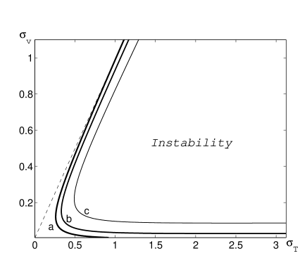
where we introduced parameters and defined by
| (40) |
Note that the parameters . For the -correlated in time random compressible velocity field . Figure 1 shows the range of parameters for in the case of (curve c), (curve b) and (curve a). The dashed line corresponds to the -correlated in time random compressible velocity field. This is a limiting line for the curve ”a”. Figure 1 demonstrates that even a very small deviations from the -correlated in time random compressible velocity field results in the instability of the second moment of the number density of inertial particles. The minimum value of required for the clustering instability is and a corresponding value of (see Fig. 1). For smaller value of the clustering instability can occur, but it requires larger values of
Notably, in Model II of a random velocity field (i.e., the Gaussian velocity field with a small yet finite correlation time) the clustering instability occurs when (see Appendix C). Indeed, the growth rate of the second moment of particles number density is determined by equation:
where St is the Strouhal number, and
Figure 2 shows the range of parameters for (curve c), (curve b) and (curve a).
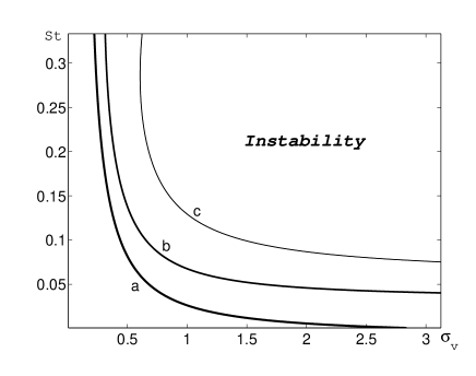
It is seen from FIG. 2 that for the second-order correlation function of the number density of inertial particles can grow in time exponentially (i.e., even for very small Strouhal numbers. For example, in the vicinity of the growth rate of the clustering instability of the second-order correlation function is given by
| (41) |
The sufficient condition for the exponential growth of the second moment of a number density of inertial particles is where the critical Schmidt number is given by The clustering instability occurs when the degree of compressibility of particles velocity i.e., for particles and droplets with the radius m . Equation (27) also yields a similar value for the threshold of the instability of the 2nd moment (at ). Note that Eq. (34) is written for .
IV Nonlinear effects
The compressibility of the turbulent velocity field with a finite correlation time can cause the exponential growth of the moments of particles number density. This small-scale instability results in formation of strong inhomogeneities (clusters) in particles spatial distributions. The linear analysis does not allow to determine a mechanism of saturation of the clustering instability. As can be seen from Eq. (39) molecular diffusion only depletes the growth rates of the clustering instability at the linear stage (contrary to the instability discussed in Ref. BF01 ). The clustering instability is saturated by nonlinear effects.
Now let us discuss a mechanism of the nonlinear saturation of the clustering instability using on the example of atmospheric turbulence with characteristic parameters: mm, s. A momentum coupling of particles and turbulent fluid is essential when , i.e., the mass loading parameter is of the order of unity (see, e.g., CST98 ). This condition implies that the kinetic energy of fluid is of the order of the particles kinetic energy where . This yields:
| (42) |
For water droplets . Thus, for m we obtain cm-3 and the total number of particles in the cluster of size , . This values may be considered as a lower estimate for the “two-way coupling” when the effect of fluid on particles has to be considered together with the feed-back effect of the particles on the carrier fluid. However, it was found in 02LP that turbulence modification by particles is governed by the ratio of the particle energy and the total energy of the suspension (rather then the energy of the carrier fluid) and thus by parameter (rather then by itself). Thus we expect that the two-way coupling can only mitigate but not stop the clustering instability.
An actual mechanism of the nonlinear saturation of the clustering instability is “four way coupling” when the particle-particle interaction is also important. In this situation the particles collisions result in effective particle pressure which prevents further grows of concentration. Particles collisions play essential role when during the life-time of a cluster the total number of collisions is of the order of number of particles in the cluster. The rate of collisions can be estimated as . The relative velocity of colliding particles with different but comparable sizes can be estimated as . Thus the collisions in clusters may be essential for
| (43) |
where is a mean separation of particles in the cluster. For the above parameters (m) cm-3, m and . Note that the mean number density of droplets in clouds is about cm-3. Therefore the clustering instability of droplets in the clouds increases their concentrations in the clusters by the orders of magnitude.
In all our analysis we have neglected the effect of sedimentation of particles in gravity field which is essential for particles of the radius m. Taking we assumed implicitly that . This is valid (for the atmospheric conditions) if m. Otherwise the cluster size can be estimated as .
Our estimates support the conjecture that the clustering instability serves as a preliminary stage for a coagulation of water droplets in clouds leading to a rain formation.
V Discussion
In this study we investigated the clustering instability of the spatial distribution of inertial particles advected by a turbulent velocity field. The instability results in formation of clusters, i.e., small-scale inhomogeneities of aerosols and droplets. The clustering instability is caused by a combined effect of the particle inertia and finite correlation time of the velocity field. The finite correlation time of the turbulent velocity field causes the compressibility of the field of Lagrangian trajectories. The latter implies that the number of particles flowing into a small control volume in a Lagrangian frame does not equal to the number of particles flowing out from this control volume during a correlation time. This can result in the depletion of turbulent diffusion.
The role of the compressibility of the velocity field is as follows. Divergence of the velocity field of the inertial particles The inertia of particles results in that particles inside the turbulent eddies are carried out to the boundary regions between the eddies by inertial forces (i.e., regions with low vorticity and high strain rate). For a small molecular diffusivity [see Eq. (1)]. Therefore, Thus there is accumulation of inertial particles (i.e., in regions with Similarly, there is an outflow of inertial particles from the regions with This mechanism acts in a wide range of scales of a turbulent fluid flow. Turbulent diffusion results in relaxation of fluctuations of particles concentration in large scales. However, in small scales where turbulent diffusion is small, the relaxation of fluctuations of particle concentration is very weak. Therefore the fluctuations of particle concentration are localized in the small scales.
This phenomenon is considered for the case when density of fluid is much less than the material density of particles When the results coincide with those obtained for the case except for the transformation where
For the value Thus there is accumulation of inertial particles (i.e., in regions with the minimum pressure of a turbulent fluid since In the case we used the equation of motion of particles in fluid flow which takes into account contributions due to the pressure gradient in the fluid surrounding the particle (caused by acceleration of the fluid) and the virtual (”added”) mass of the particles relative to the ambient fluid MR83 .
The exponential growth of the second moment of a number density of inertial particles due to the small-scale instability can be saturated by the nonlinear effects (see Section IV). The excitation of the second moment of a number density of particles requires two kinds of compressibilities: compressibility of the velocity field and compressibility of the field of Lagrangian trajectories, which is caused by a finite correlation time of a random velocity field. Remarkably, the compressibility of the field of Lagrangian trajectories determines the coefficient of turbulent diffusion (i.e. the coefficient near the second-order spatial derivative of the second moment of a number density of inertial particles in Eq. (29). The compressibility of the field of Lagrangian trajectories causes depletion of turbulent diffusion in small scales even for . On the other hand, the compressibility of the velocity field determines a coefficient B(r) near the second moment of a number density of inertial particles in Eq. (29). This term is responsible for the exponential growth of the second moment of a number density of particles.
Summary:
We showed that the physical reason for the clustering instability in spatial distribution of particles in turbulent flows is a combined effect of the inertia of particles leading to a compressibility of the particle velocity field and a finite velocity correlation time.
The clustering instability can result in a strong clustering whereby a finite fraction of particles is accumulated in the clusters and a weak clustering when a finite fraction of particle collisions occurs in the clusters.
The crucial parameter for the clustering instability is a radius of the particles . The instability criterion is for which . For the droplets in the atmosphere m. The growth rate of the clustering instability , where is the turnover time in the viscous scales of turbulence.
We introduced a new concept of compressibility of the turbulent diffusion tensor caused by a finite correlation time of an incompressible velocity field. For this model of the velocity field, the field of Lagrangian trajectories is not divergence-free.
We suggested a mechanism of saturation of the clustering instability - particle collisions in the clusters. An evaluated nonlinear level of the saturation of the droplets number density in clouds exceeds by the orders of magnitude their mean number density.
Acknowledgements.
We have benefited from discussions with I. Procaccia. This work was partially supported by the German-Israeli Project Cooperation (DIP) administrated by the Federal Ministry of Education and Research (BMBF), by the Israel Science Foundation and by INTAS (Grant 00-0309). DS is grateful to a special fund for visiting senior scientists of the Faculty of Engineering of the Ben-Gurion University of the Negev and to the Russian Foundation for Basic Research (RFBR) for financial support under grant 01-02-16158.Appendix A Basic equations in the model with a random renewal time
In this Appendix we derive Eq. (63) for the simultaneous second-order correlation function which serves as a basis for further analysis in Appendixes B and C under some simplifying model assumptions about the statistics of the velocity field.
SSmethodExact solution of dynamical equations for a given velocity field
A.0.1 Simple case: no molecular diffusion
Consider first Eq. (1) for the number density of particles in the case :
| (44) |
when all particles are transported only by advection. Solution of Eq. (44) with the initial condition is given by
| (45) |
where is the Lagrangian trajectory of the particle which is located at coordinate at time . Here we label the particles at present moment of time and consider a current time as moments in the past. This differs from a usual approach, see Eqs. LABEL:rL, when particles are labelled at the initial time , and a current time . Therefore in the equations below it is more convenient to redefine Lagrangian displacement . Now Eqs. LABEL:rL can be written as
| (46) | |||||
| (47) |
The Green function is the functional of :
| (48) |
Introduce the shift operator
| (49) |
which acts as follows:
| (50) |
One can validate relation LABEL:shift1 by Taylor series expansion of the function . Now Eq. (45) can be rewritten as follows:
| (51) |
A.0.2 Molecular diffusion as a Wiener process
Consider now the full Eq. (1) with whereby particles are transported by both, fluid advection and molecular diffusion. It was found by Wiener (see, e.g., ZRS90 ) that Brownian motion (molecular diffusion) can be described by the Wiener random process with the following properties:
| (52) |
Here denotes the mathematical expectation over the statistics of the Wiener process. Introduce the Wiener trajectory (which usually is called the Wiener path) and the Wiener displacement as follows:
| (53) | |||||
Comparison of this formula with Eqs. LABEL:rL1 shows that in the limit , and .
In Refs. [EKR00, ] it was shown that solution of Eq. (1) (with ) can be written as solution LABEL:A4 of Eq. (44) (with ) by replacement and then averaging over the statistics of the Wiener processes LABEL:W:
| (54) |
SSvelocityTwo-step averaging over velocity statistics
A.0.3 Model of a random velocity field
Note that Eq. (54) is a solution of Eq. (1) at a given realization of the random velocity field. Our next goal is to determine the simultaneous correlation functions
| (55) | |||||
averaged over the stationary, space homogeneous statistics of turbulent velocity field, where denotes this averaging. Since the initial distribution is assumed to be homogeneous in space, is independent of spatial coordinate, and depends only on the difference .
In order to simplify the averaging procedure LABEL:def-cor we consider a model of random velocity field which fully looses memory at some instants of renewal . For and inside a renewal interval [] the velocity pair correlation function is defined as
| (56) |
where denotes averaging over “intrinsic statistics” of the velocity field. In our model the velocity fields before and after renewals are statistically independent. The interval between the renewal instants may be the same or randomly distributed, say with the Poisson statistics. In the latter case the full averaging may be considered as a two-stage process. First one calculates and then averages over the statistics of the renewal time , which is denoted as :
| (57) |
For the Poisson statistics of
| (58) | |||||
where is a mean renewal time. It would be useful to define the correlation time of the function as follows
| (59) |
Certainly this model of the random velocity field cannot be considered as universal. However, it reproduces important features of some flows (see, e.g., Ref. [LST00, ]).
A.0.4 Averaging procedure
Our model involves three random processes:
-
1.
The Wiener random process which describes Brownian (molecular) diffusion.
-
2.
Poisson process for a random renewal time.
-
3.
The random velocity field between the renewals.
Eq. (54) presents after the first step, i.e., it describes the number density at a given realization of a velocity field. Using Eq. (54) we obtain
| (60) |
where and and denotes averaging over two independent Wiener processes determining two Wiener paths. Hereafter for simplicity we use the following notations: and
Now we average Eq. (60) over a random velocity field for a given realization of a Poisson process:
Here the time is the last renewal time before time and is a random variable. Thus, averaging of the functions
is decoupled into two time intervals because the first function is determined by the velocity field after the renewal while the second function is determined by the velocity field before renewal. Now we take into account that for the Poisson process any instant can be chosen as the initial instant. We average Eq. (A.0.4) over the random renewal time. The probability density for a random renewal time is given by
| (62) |
Thus the resulting averaged equation for “fully” averaged correlation function , defined by Eq. (55), assumes the following form:
| (63) |
The first term in Eq. (63) describes the case when there is at least one renewal of the velocity field during the time (i.e., the Poisson event), whereas the second term describes the case when there is no renewal during the time . Here and
| (64) | |||
where . Equation LABEL:C14 is simplified in Appendixes B and C under the additional assumptions about the velocity field statistics.
Appendix B velocity field with Gaussian Lagrangian trajectories
Consider a model of a random velocity field where Lagrangian trajectories, i.e., the integrals and have Gaussian statistics. Using an identity in Eq. (64) we obtain
| (65) |
where
| (66) | |||||
Here is a Gaussian random variable with zero mean value and unit variance and The latter yields
where When correlation time , Eq. (59), is much less then the current time and , these correlation functions are given by
| (67) | |||||
where we used an identity
Eq. (65) allows to rewrite Eq. (63) as
| (68) | |||||
where
| (69) |
To derive Eq. (68) we used the following identity
| (70) |
which follows from the Taylor expansion
| (71) |
In particular,
Evaluating the integral in Eq. (68) we obtain
| (72) |
Here we used the commutativity relation
Thus, finally
| (73) |
Note that in the limit , Eq. (73) describes the evolution of in the model of the random velocity field without renewals.
Appendix C Gaussian velocity field with a small yet finite correlation time
Here we consider a random Gaussian velocity field with a small . Using Eq. (70) we rewrite Eq. (63) in the form
| (74) |
where and we neglected the last term in Eq. (63) for small . Expanding the function in Taylor series in the vicinity of we obtain
| (75) |
where we used that
Neglecting the terms in Eq. (75) we obtain
where we used that the expansion of the operator into Taylor series (for small for a random Gaussian velocity field has only even powers of Thus, the equation for the correlation function is given by
| (77) |
where
| (78) | |||||
| (79) | |||||
| (80) |
Here for the homogeneous turbulent velocity field EKRS99 :
Using the expansion of and into Taylor series of a small time after the lengthly algebra we obtain
| (81) | |||||
| (82) | |||||
| (83) | |||||
| (84) | |||||
and St is the Strouhal number. In these calculations we neglected small terms Our analysis showed that the neglected small terms do not affect the growth rate of the clustering instability. In Eqs. (82)-(84) we assumed that the correlation function for homogeneous, isotropic and compressible velocity field is given by
| (85) |
(see EKR95 ), and in scales incompressible and compressible components of the random velocity field are given by
in scales the functions Here is measured in the units of and Turbulent diffusion tensor is determined by the field of Lagrangian trajectories [see Eq. (78)]. Due to a finite correlation time of a random velocity the field of Lagrangian trajectories is compressible even if the velocity field is incompressible Indeed, for we obtain
Using Eqs. (81)-(85) we calculate the functions and
| (86) | |||||
| (87) | |||||
| (88) |
where and
We will show here that the combined effect of particles inertia and finite correlation time results in the excitation of the clustering instability whereby under certain conditions there is a self-excitation of the second moment of a number density of inertial particles. This instability causes formation of small-scale inhomogeneities in spatial distribution of inertial particles.
The equation for the second-order correlation function for the number density of inertial particles reads
| (89) |
[see Eqs. (88)], where the time is measured in units of and
In order to obtain a solution of Eq. (89) we use a separation of variables, i.e., we seek for a solution in the following form:
whereby is a free parameter which is determined using the boundary conditions
Here is measured in units of . Since the function is the two-point correlation function, it has a global maximum at and therefore it satisfies the conditions:
Then Eq. (89) yields
| (90) |
where . Equation (90) has an exact solution for
| (91) | |||||
and and are the Legendre functions with imaginary argument
Solution of Eq. (89) can be analyzed using asymptotics of the exact solution (91). This asymptotic analysis is based on the separation of scales (see, e.g., ZMR88 ; EKR95 ). In particular, the solution of Eq. (89) has different regions where the form of the functions and are different. The functions and in these different regions are matched at their boundaries in order to obtain continuous solution for the correlation function. Note that the most important part of the solution is localized in small scales (i.e., Using the asymptotic analysis of the exact solution for allowed us to obtain the necessary conditions of a small-scale instability of the second moment of a number density of inertial particles. The results obtained by this asymptotic analysis are presented below.
The solution (91) has the following asymptotics: for (i.e., in the scales the solution for the second moment is given by
| (92) |
For (i.e., in the scales the function is given by
| (93) |
When the second-order correlation function for a number density of inertial particles is given by
where and is the argument of the complex constant For the second-order correlation function for the number density of inertial particles is given by
| (94) |
where . Since the total number of particles in a closed volume is conserved, i.e., particles can only be redistributed in the volume,
The latter yields for and When , the solution (93) cannot be matched with solutions (92) and (94). Thus, the condition is the necessary condition for the existence of the solution for the correlation function. The condition provides the existence of the global maximum of the correlation function at .
Matching functions and at the boundaries of the above-mentioned regions yields coefficients and In particular, the eigenvalue is given by Eq. (III.2).
References
- (1) C.T. Crowe, M.Sommerfeld and Y.Tsuji, Multiphase flows with particles and droplets (CRC Press, NY, 1998), and references therein.
- (2) S. Twomey, Atmospheric Aerosols ( Elsevier Scientific Publication Comp., Amsterdam, 1977), and references therein.
- (3) G. T. Csanady, Turbulent Diffusion in the Environment (Reidel, Dordrecht, 1980), and references therein.
- (4) J. H. Seinfeld, Atmospheric Chemistry and Physics of Air Pollution, (John Wiley, New York, 1986), and references therein.
- (5) T. Elperin, N. Kleeorin , M. Podolak and I. Rogachevskii, Planetary and Space Science 45, 923 (1997), and references therein.
- (6) R. A. Shaw, W. C. Reade, L. R. Collins and J. Verlinde, J. Atmos. Sci. 55, 1965 (1998).
- (7) T. Elperin, N. Kleeorin and I. Rogachevskii, Int. J. Multiphase Flow 24, 1163 (1998); Atmos. Res. 53, 117 (2000) and references therein.
- (8) P. A. Vaillancourt and M. K. Yau, Bull. Americ. Meteorol. Soc. 81, 285 (2000), and references therein.
- (9) K. Annamalai and W. Ryan, Prog. Energy Combust. 18, 221 (1992).
- (10) K. Annamalai, W. Ryan and S. Dhanapalan, Prog. Energy Combust. 20, 487 (1994).
- (11) I. R. Paluch and D. G. Baumgardner, J. Atmos. Sci. 46, 261 (1989), and references therein.
- (12) A. V. Korolev and I. P. Mazin, J. Applied Meteorology 32, 760 (1993), and references therein.
- (13) B. Baker and J.-L. Brenguier, Proc. American Meteorology Society on Cloud Physics, Everett, Washington, 148 (1998).
- (14) A. B. Kostinski and R. A. Shaw, J. Fluid Mech. 434, 389 (2001).
- (15) K. D. Squires and J. K. Eaton, Phys. Fluids A3, 1169 (1991).
- (16) J. K. Eaton and J. R. Fessler, Int. J. Multiphase Flow 20, (Suppl) 169 (1994).
- (17) J. R. Fessler, J. D. Kulick, and J. K. Eaton, Phys. Fluids 6, 3742 (1994).
- (18) F. Hainaux, A. Aliseda, A. Cartellier, and J. C. Lasheras, Advances in Turbulence VIII, Proc. VIII Europ. Turbulence Conference, Barcelone 2000, C. Dopazo et al. (eds), 553 (2000).
- (19) T. Elperin, N. Kleeorin and I. Rogachevskii, Phys. Rev. Lett. 77, 5373 (1996).
- (20) T. Elperin, N. Kleeorin, I. Rogachevskii and D. Sokoloff, Phys. Chem. Earth A 25, 797 (2000).
- (21) T. Elperin, N. Kleeorin, I. Rogachevskii and D. Sokoloff, Phys. Rev. E 63, 046305 (2001).
- (22) R. H. Kraichnan, Phys. Fluids 11, 945 (1968).
- (23) V.S. L’vov and I. Procaccia, Phys. Rev. E, 52, 3858 (1995).
- (24) V.S. L’vov and I. Procaccia, Phys. Rev. E, 52, 3840 (1995).
- (25) M. R. Maxey, J. Fluid Mech. 174, 441 (1987).
- (26) M. R. Maxey and S. Corrsin, J. Atmos. Sci. 43, 1112 (1986).
- (27) L. P. Wang and M. R. Maxey, J. Fluid Mech. 256, 27 (1993).
- (28) M. R. Maxey, E. J. Chang and L.-P. Wang, Experim. Thermal and Fluid Science 12, 417 (1996).
- (29) T. Elperin, N. Kleeorin and I. Rogachevskii, Phys. Rev. Lett. 76, 224 (1996); 80, 69 (1998); 81, 2898 (1998).
- (30) E. Balkovsky, G. Falkovich and A. Fouxon, Phys. Rev. Lett. 86, 2790 (2001).
- (31) S. F. Shandarin and Ya. B. Zeldovich, Rev. Mod. Phys. 61, 185 (1989).
- (32) V. I. Klyatskin and A. I. Saichev, JETP 84, 716 (1997).
- (33) Ya. B. Zeldovich, A. A. Ruzmaikin, and D. D. Sokoloff, The Almighty Chance (Word Scientific Publ., Singapore, 1990), and references therein.
- (34) Ya. B. Zeldovich, S. A. Molchanov, A. A. Ruzmaikin and D. D. Sokoloff, Sov. Sci. Rev. C. Math Phys. 7, 1 (1988), and references therein.
- (35) T. Elperin, N. Kleeorin, I. Rogachevskii and D. Sokoloff, Phys. Rev. E 61, 2617 (2000); 64, 026304 (2001).
- (36) T. Elperin, N. Kleeorin and I. Rogachevskii, Phys. Rev. E 52, 2617 (1995).
- (37) G. I. Taylor, Proc. London Math. Soc. 20, 196 (1921).
- (38) V. S. L’vov and A. Pomyalov, One-fluid description of turbulently flowing suspensions, Phys. Rev. Lett., submitted. Also: nlin.CD/0203016
- (39) M. R. Maxey and J. J. Riley, Phys. Fluids 26, 883 (1983).
- (40) V. G. Lamburt, D. D. Sokoloff and V. N. Tutubalin, Astron. Rep., 44, 659 (2000).