Does ohmic heating influence the flow field in thin-layer electrodeposition?

Abstract

In thin-layer electrodeposition the dissipated electrical energy leads to a substantial heating of the ion solution. We measured the resulting temperature field by means of an infrared camera. The properties of the temperature field correspond closely with the development of the concentration field. In particular we find, that the thermal gradients at the electrodes act like a weak additional driving force to the convection rolls driven by concentration gradients.

I Introduction

The electrochemical deposition of metals from aqueous solutions in quasi-two-dimensional geometries has proven to be a valuable test bed to examine concepts of interfacial growth like fractal growth Argoul et al. (1988); Kuhn and Argoul (1995), morphological transitions Fleury et al. (1991); Kuhn and Argoul (1994); Lòpez-Salvans et al. (1997) or dendritic growth Barkey et al. (1995); Argoul et al. (1996). The properties of the evolving deposit are in many cases sensitive to the presence of convection currents in the solution Jorne et al. (1987); López-Tomàs et al. (1993); Barkey et al. (1994); Lòpez-Salvans et al. (1996); Rosso et al. (1999); Schröter et al. (2002). There are two well-known origins of convection rolls: a) on small scales, spatial inhomogeneities of the ionic charge distribution can trigger electro-convection Fleury et al. (1992, 1993); Huth et al. (1995); b) density inhomogeneities due to concentration changes at the electrodes induce large scale gravity-driven convection rolls Rosso et al. (1994); Barkey et al. (1994); Huth et al. (1995); Linehan and de Bruyn (1995); Chazalviel et al. (1996); Argoul et al. (1996); Dengra et al. (2000); Schröter et al. (2002).

However there is another potential source of density changes: due to the small cell volume of typically $\leq$ 1 $\rm cm^{3}$, the dissipated electric energy can be the source of a significant heating. If the cell were completely thermally insulated, a solution exposed to an electrical power of 500 mW would start to boil after 500 s. While thermal conduction will confine the overall temperature increase to smaller values, considerable temperature gradients might arise and generate density driven convection.

Thermally induced convection rolls have been thoroughly studied in thin-layer geometries heated from below (for a recent review see Bodenschatz et al. (2000)) and the side Cormack et al. (1974); Imberger (1974); Patterson and Imberger (1980); Boehrer (1997); Delgado-Buscalioni (2001). In contrast, the role of thermal effects was previously not examined in electrodeposition. In order to quantify the possible temperature gradients, a high spatial resolution of the temperature field is necessary. We present here measurements of the temperature field at both electrodes performed by use of an infrared camera. The so determined evolution of the temperature field can be related to the development of the concentration field, which is known from interferometric measurements Argoul et al. (1996); Léger et al. (2000). The remainder of the paper is organized as follows: Section II describes our experimental setup, section III presents the measurement results, which will be discussed in sec. IV.

II Experimental Setup

The measurements are performed with the infrared camera Varioscan 3021-ST from InfraTec, which contains a Stirling-cooled HgCdTe-detector with 360 $\times$ 240 pixel. Using its macro we observe an area of 5.0 $\times$ 3.4 $\rm cm^{2}$, which yields a spatial resolution of 140 $\mu$m. The maximal image capturing frequency is 1.1 Hz, the thermal resolution $\pm$ 30 mK.

While the sensor is sensitive for wavelengths in the range of 8-12 $\mu$m, glass plates, which are normally used as top and bottom plate of the cell, are opaque in this region. Therefore the upper cell cover was realized using a polyethylene foil stretched over an aluminium frame. Due to the flexibility of the polyethylene foil and a small overpressure necessary to fill the cell, the plate separation of about 0.5 mm is not well defined. The bottom plate of the cell consists of a block of Teflon, because this material has a low reflectivity in the infrared. This reduces the so called narcissism: the response of the cooled detector to its own mirror image. The electrodes are parallel zinc wires (Goodfellow 99.99%) of 0.25 mm diameter and separated by a distance of 4 cm. Fig.1 shows an image of the cell during an experiment.

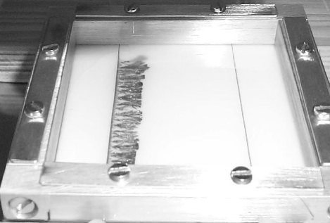
Figure 1: Cell used for the infrared measurements. The bottom (white) consists of Teflon, the upper cover is a polyethylene foil stretched over an aluminium frame. The electrodes are parallel zinc wires with a distance of 4 cm. The deposit at the cathode has grown for 410 s.

The cell is filled with an 0.1 M $\rm ZnSO_{4}$ solution prepared from Merck p.a. chemicals in nondeaerated ultrapure $\rm H_{2}O$. The measurements are performed at a constant potential of 20 $\pm$ 0.003 V. Due to the current increase during the electrodeposition process, the average electrical power feed $\dot{Q}_{\rm el}$ increases from 470 mW at the beginning of the experiment to 650 mW after 500 s.

Because of the modified cell construction, the question of comparability with experiments performed in standard electrodeposition cells could be raised. Therefore we calculate the heat-flux $k_{i}A_{i}$ for the confining plates, where $A_{i}$ and $k_{i}$ are the area and the heat transfer coefficient of the plate. It is important to keep in mind, that $1/k_{i}$ is equivalent to $1/\alpha_{1}+1/\alpha_{2}+\Delta z_{i}/\lambda_{i}$. Here $\alpha_{1}$ and $\alpha_{2}$ are the heat transition numbers from solution to plate resp. plate to air, $\lambda_{i}$ is the heat conductivity and $\Delta z_{i}$ the thickness of the plate.

Inserting the material parameters of our setup James and Lord (1992); Lindner (1989) and using only the area between the two electrodes, we derive a $k_{i}A_{i}$ of 16.2 mW per Kelvin temperature difference for the polyethylene foil and 11.5 mW/K for the Teflon plate, while a typical glass plate (Schott BK 7, 6.3 mm thick) yields 16 mW/K. So in a first approximation our setup is thermally equivalent to a standard electrodeposition cell.

III Experimental Results

Fig. 1 shows the growing deposit at the cathode, which belongs to the homogenous morphology Sagués et al. (2000). It is characterized by tip-splitting but retaining a growing front parallel to the cathode. After 500 s a Hecker transition Kuhn and Argoul (1994) takes place and the growth front breaks up into more spatially localized zones of active development.

Immediately before each experiment the infrared camera takes a zero image, which is then subtracted from all images taken during the experiment. Therefore the thermographies solely depict the temperature increase. Fig. 2 gives an example of such a thermography after 280 s, the scale at the right describes the temperature increase with respect to the beginning of the experiment. The white line marks the position of the anodic zinc wire. The temperature decrease at the left hand side of the image is caused by the thermal conductivity of the aluminium frame, the warm “island” in the middle is due to the inhomogeneity of the cell thickness.

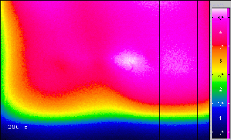
Figure 2: Thermography taken 280 s after the start of the experiment. The size of the image is 5.0 $\times$ 3.4 $\rm cm^{2}$. The white line corresponds to the position of the anodic zinc wire, the rows between the black lines are averaged to produce Fig. 3.

In order to improve the signal to noise ratio, zones of spatial homogeneity and a width of 9.1 mm are chosen by visual inspection. Such a zone is depicted in Fig. 2 with two parallel black lines. Inside this zone all rows are averaged, yielding a temperature increase $\Delta T(y,t)$, which is only a function of distance to the cathode $y$ and time.

Fig. 3 shows the evolution of $\Delta T$ in the neighborhood of the anode. It is clearly visible that the temperature increase at the anode itself lags behind with respect to the one observed in the middle of the cell.

Figure 3: Temporal evolution of the temperature field at the anode, which is located at 40 mm. All data are averaged over a width of 9.1 mm. The arrows indicate the position where the deviation of $\Delta T$ from the bulk temperature becomes less than 20 mK.

Fig. 4 illustrates the evolution of the temperature field at the cathode. The most prominent feature is the existence of a local temperature maximum, denoted with small arrows. This maximum moves towards the middle of the cell, where a plateau of spatially constant temperature is located.

Figure 4: Temporal evolution of the temperature field at the cathode. All data are averaged over a width of 9.1 mm. The arrows mark the position of the temperature maximum.

In order to characterize the heating process in the cell, we pick the temperature at a distance of 25.6 mm to the cathode (this is approximately the location, where the two convection rolls emerging from the electrodes finally meet, as will be discussed in Section IV.2). Referring to this point, we will speak of the bulk in the following. In Fig. 5 this temperature increase $\Delta T_{\rm bulk}$ is given for the two experiments presented in Fig. 3 and 4. The fact that the two measurements are almost identical reflects the reproducibility of the experiment. The solid line is a fit to an exponential function, which is motivated in detail in Section IV.3.

Figure 5: Temperature increase in the bulk of the cell at a distance of 14.4 mm to the anode and 25.6 mm to the cathode. The $\circ$ correspond to the experiment presented in Fig. 4 the $\blacksquare$ to the one in Fig. 3. The solid line is a fit of Equation 5 to the $\circ$.

The arrows in Fig. 3 represent the location, where the temperature is 20 mK smaller than $\Delta T_{\rm bulk}$. The distance of these points with respect to the anode is denoted $L_{a}(t)$ and is shown in Fig. 6 (a). Its monotonous increase with time is fitted by a power law, which will be explained in Section IV.1. Correspondingly, Fig. 6 (b) shows the growth of the distance $L_{c}(t)$ between the the location of the temperature maximum in Fig. 4 and the cathode. The straight line is a fit to all data with $t>$ 100 s, which will be motivated in Sec. IV.2.

Figure 6: Temporal evolution of: (a) the distance between the anode and the point, where the temperature starts to deviate from the bulk. The solid line is a fit with Equation 1. (b) the distance between the temperature maximum and the initial cathode position. The fit is performed with Equation 2 to the data indicated with filled symbols.

IV Discussion and conclusions

In principle, the energy balance involves three contributions: the electrical energy feed into the cell, the dissipated ohmic heat and the chemical reaction energy. However the short calculation presented in the appendix supports the assumption that the chemical energy contribution is mostly irrelevant.

The ohmic heat dissipated at some position in the cell will be proportional to the local resistivity $\rho(y,t)$ in a one-dimensional model, while $\rho$ will depend on the local ion concentration $c(y,t)$. In the next three subsections we will compare the evolution of the temperature field at the anode, at the cathode and in the bulk with the development of the concentration field, which is known from interferometric measurements Argoul et al. (1996); Léger et al. (2000).

IV.1 Evolution of the temperature field at the anode

At the anode $\rm Zn^{2+}$ ions go into solution, increasing the local concentration and therefore density. While this denser solution sinks down to the bottom plate, it gets replaced by less dense bulk solution. This mechanism drives a convection roll of size $L$ Huth et al. (1995); Chazalviel et al. (1996); Schröter et al. (2002). According to the fluid dynamical description there are two growth regimes: Initially during the so called immiscible fluid regime $L$ will grow with $t^{0.8}$, while after some time there will be a crossover to the diffusion hindered spreading regime with a $t^{0.5}$ growth law. Chazalviel et al. Chazalviel et al. (1996) showed, that both the fluid velocity $v$ and the ion concentration decrease with increasing distance to the electrode. The distance, where $v$ has dropped to zero and coincidently $c$ has fallen to $c_{\rm bulk}$, defines $L$.

Figure 3 shows that the temperature increase in the region between the anode and the arrows lags behind the one observed in the bulk. As $c>c_{\rm bulk}$ translates into reduced ohmic heating, we identify the position of the arrows with the end of the anodic convection roll. A fit to its length with:

$$L_{\rm a}(t)=at^{b}$$ (1)

is presented in Fig 6 (a). It yields: a = 0.13 $\pm$ 0.01 mm and b = 0.78 $\pm$ 0.01, which indicates that the convection roll is in the immiscible fluid regime for the whole run of the experiment. According to the scaling analysis presented in Ref. Schröter et al. (2002), this corresponds to an average plate separation of about 650 $\mu$m.

IV.2 Evolution of the temperature field at the cathode

Due to the growing deposit, there is a zone of ion depletion in the vicinity of the cathode, the size of which will be affected by the convection roll driven by the occuring density difference. As the decreased $c$ leads to higher dissipation, the increased temperature denoted by the arrows in Fig. 4 is qualitatively explained. The distance of the arrows to the initial cathode position $L_{\rm c}(t)$ should correspond to the actual size of the deposit. Therefore we perform a linear fit with:

$$L_{\rm c}(t)=v_{\rm c}t+l_{\rm c}$$ (2)

which is shown in Fig. 6 (b). We derive $v_{\rm c}$ = 21.2 $\pm$ 0.4 $\mu$m/s, which agrees well with 20.7 $\pm$ 0.8 $\mu$m/s front velocity determined from photographs of the deposit.

$l_{\rm c}$ is found to be 2 $\pm$ 0.1 mm. This finite distance can be explained by the absence of heat production in the metallic deposit because of its low resistivity and the fact that its heat conductivity is 190 times higher than water. So the deposit is an effective heat sink, the resulting heat flux shifts the temperature maximum into the cell.

If the cathodic convection roll, apart from the fact that it starts at the actual front of the deposit, grows in the same way as the anodic roll, they meet 450 s after the beginning of the experiment at a distance of 25 mm to the cathode. This corresponds to the observed change in morphology after that time.

IV.3 Temperature evolution in the bulk

The temperature increase observed in Fig. 5 can be modeled, if we assume, that the whole cell shares the constant bulk properties $c$ and $\rho$ and therefore $T$. The supplied electrical power $\dot{Q}_{\rm el}$ would then be compensated by the heating of the system with heat capacity $C$ and the heat flow $\dot{Q}_{\rm flow}$:

$$\dot{Q}_{\rm flow}=-(T-T_{0})\sum_{i}k_{i}A_{i}$$ (3)

where $T_{0}$ represents the ambient temperature and $T$ the temperature inside the electrolyte. If we assume $\dot{Q}_{\rm el}$ to be constant, the corresponding differential equation:

$$\dot{Q}_{\rm el}=(T-T_{0})\sum_{i}k_{i}A_{i}+C\frac{\partial T}{\partial t}$$ (4)

has the straightforward solution:

$$(T-T_{0})=T_{\rm final}\left(1-e^{\nicefrac{{-t}}{{\tau}}}\right)$$ (5)

Here $T_{\rm final}=\dot{Q}_{\rm el}/\sum_{i}k_{i}A_{i}$ denotes the finally reached temperature difference and $\tau=C/\sum_{i}k_{i}A_{i}$ is the time constant of the heating up. A fit of Equation 5 to the experimental data is displayed in Fig. 5. It yields: $T_{\rm final}$ = 9 $\pm$ 0.2 K. This translates to an overall heat-flux $\sum_{i}k_{i}A_{i}$ of 60 mW per K temperature difference. A comparison of this result with the values of $k_{i}A_{i}$ calculated in Sec. II shows that about 50% of the heat flux takes place through the top and the bottom plate of the cell. The heat flux through the side walls, the electrodes and the plate area beyond the electrodes accounts for the rest.

IV.4 Influence of the temperature gradients on the convection rolls

In order to estimate the influence of the temperature gradients on the concentration driven convection currents, we plot in Fig. 7 the difference between $\Delta T_{\rm bulk}$ and a) the cathodic temperature maximum and b) the anode. These temperature gradients result in a down-flow at the anode and an up-flow at the growth front, so they act as an additional driving.

Figure 7: Temperature difference between the bulk and $\circ$: the cathodic temperature maximum and $\blacksquare$: the temperature at the anode.

Figure 8: Temperature dependency of the densities at the anode and in the bulk. The $\bullet$ correspond to $c$ = 1.0 m $\rm ZnSO_{4}$, the $\circ$ to $c_{\rm bulk}$ = 0.1 m $\rm ZnSO_{4}$.

For a more quantitative determination of their contribution, the temperature dependency of the density was measured for different concentrations. The applied density measurement instrument DMA 5000 from Anton Paar has an accuracy better than 50 $\mu$g/$\rm cm^{3}$.

After 400 s the temperature of the 0.1 M $\rm ZnSO_{4}$ bulk solution has reached about 30 ^∘ C which corresponds to a density of 1012.3 mg/$\rm cm^{3}$. In accordance with the measurements presented in Ref. Argoul et al. (1996) and the theory in Ref. Chazalviel et al. (1996), we estimate $c$ at the anode for that time as 0.25 M. This corresponds to a density of 1036.4 mg/$\rm cm^{3}$ for $T$ = 30 ^∘ C and 1037.4 mg/$\rm cm^{3}$ for the actually measured $T\approx$ 27 ^∘ C. So the contribution of the temperature gradient to the overall density difference at the anode is about 4% as visualized in Fig. 8.

At the cathode $c$ has reached zero at that time, $\rho$ of $\rm H_{2}O$ is 995.68 mg/$\rm cm^{3}$ for $T$ = $30^{\circ}$ C and 995.38 mg/$\rm cm^{3}$ for the $T$ = $31^{\circ}$ C at the maximum. This results in a 2% contribution of the temperature gradient to the total density contrast.

As our applied potential is above average for standard electrodeposition experiments, we conclude that temperature inhomogeneities will only weakly contribute to the density driven convection rolls. This result justifies with hindsight the use of the theoretical description of Chazalviel et al.Chazalviel et al. (1996). Finally it should be remarked that morphologies like stringy Trigueros et al. (1992), where the zone of active growth is restricted to few small spots with very high local current densities, may differ substantially from our results.

V appendix

The standard enthalpy of formation $\Delta_{\rm b}H^{\ominus}$ of $\rm Zn^{2+}$ ions in an infinitely diluted solutions is $-153.89$ kJ/mol Atkins (1990). It contains three different contributions: 1) the energy necessary to liberate an atom from the surrounding lattice, 2) the energy needed to ionize the atom and 3) the hydration energy, which is set free when the water dipoles surround the ion. Only the last term depends on the concentration of the solution, decreasing with the number of ions already dissolved.

As the reaction rate at the electrodes is directly proportional to the electrical current $I$, so is the chemical power $\dot{Q}_{\rm chem}$ :

$$\dot{Q}_{\rm chem}=\frac{\Delta_{\rm b}H^{\rm\ominus}}{F\;z}\;I$$ (6)

where $F$ is the Faraday constant (96485 As/mol) and $z$ the charge number. For zinc we derive $\dot{Q}_{\rm chem}/I$ = -0.8 mW/mA. In the vicinity of the anode this number leads to additional heating due to the transformation of chemical energy. At the cathode the chemical energy stored in the newly produced zinc has to be subtracted from the overall heat production, but does not lead to a direct cooling of the cathode.

With our experimental conditions an average current of 30 mA feeds an electrical power of 600 mW into the cell. Compared to that $\dot{Q}_{\rm chem}$ is 24 mW which is about 4% of the electrical power.

At the cathode the ion concentration drops fast to zero, which justifies the approximation of an infinitely diluted solution. At the anode the ion concentration increases during the whole run of the experiment. Therefore the hydration energy of the newly produced $\rm Zn^{2+}$ ions decreases and in consequence the heat, which is released from the chemical reaction decrease as well. So the overall heat production from chemical energy at the anode is smaller than estimated here and therefore mostly irrelevant for the energy balance. This conclusion agrees with the fact that the anode is the coldest point of the cell as clearly shown in Fig 3, in spite of this extra heat production there.

References

- Argoul et al. (1988) F. Argoul, A. Arneodo, G. Grasseau, and H. L. Swinney, Phys. Rev. Lett. 61, 2558 (1988).
- Kuhn and Argoul (1995) A. Kuhn and F. Argoul, J. Electroanal. Chem. 397, 93 (1995).
- Fleury et al. (1991) V. Fleury, M. Rosso, and J.-N. Chazalviel, Phys. Rev. A 43, 6908 (1991).
- Kuhn and Argoul (1994) A. Kuhn and F. Argoul, Phys. Rev. E. 49, 4298 (1994).
- Lòpez-Salvans et al. (1997) M.-Q. Lòpez-Salvans, F. Sagués, J. Claret, and J. Bassas, Phys. Rev. E 56, 6869 (1997).
- Barkey et al. (1995) D. Barkey, F. Oberholtzer, and Q. Wu, Phys. Rev. Lett. 75, 2980 (1995).
- Argoul et al. (1996) F. Argoul, E. Freysz, A. Kuhn, C. Léger, and L. Potin, Phys. Rev. E 53, 1777 (1996).
- Jorne et al. (1987) J. Jorne, Y.-J. Lii, and K. E. Yee, J. Electrochem. Soc. 134, 1399 (1987).
- López-Tomàs et al. (1993) L. López-Tomàs, J. Claret, and F. Sagués, Phys. Rev. Lett. 71, 4373 (1993).
- Barkey et al. (1994) D. P. Barkey, D. Watt, and S. Raber, J. Electrochem. Soc. 141, 1206 (1994).
- Lòpez-Salvans et al. (1996) M.-Q. Lòpez-Salvans, P. P. Trigueros, S. Vallmitjana, J. Claret, and F. Sagués, Phys. Rev. Lett. 76, 4062 (1996).
- Rosso et al. (1999) M. Rosso, E. Chassaing, and J.-N. Chazalviel, Phys. Rev. E 59, 3135 (1999).
- Schröter et al. (2002) M. Schröter, K. Kassner, I. Rehberg, J. Claret, and F. Sagués, Phys. Rev. E 65, 041607 (2002).
- Fleury et al. (1992) V. Fleury, J.-N. Chazalviel, and M. Rosso, Phys. Rev. Lett. 68, 2492 (1992).
- Fleury et al. (1993) V. Fleury, J.-N. Chazalviel, and M. Rosso, Phys. Rev. E 48, 1279 (1993).
- Huth et al. (1995) J. M. Huth, H. L. Swinney, W. D. McCormick, A. Kuhn, and F. Argoul, Phys. Rev. E 51, 3444 (1995).
- Rosso et al. (1994) M. Rosso, J. N. Chazalviel, V. Fleury, and E. Chassaing, Elektrochimica Acta 39, 507 (1994).
- Linehan and de Bruyn (1995) K. A. Linehan and J. R. de Bruyn, Can. J. Phys. 73, 177 (1995).
- Chazalviel et al. (1996) J. N. Chazalviel, M. Rosso, E. Chassaing, and V. Fleury, J. Electroanal. Chem. 407, 61 (1996).
- Dengra et al. (2000) S. Dengra, G. Marshall, and F. Molina, J. Phys. Soc. Jpn. 69, 963 (2000).
- Bodenschatz et al. (2000) E. Bodenschatz, W. Pesch, and G. Ahlers, Annu. Rev. Fluid. Mech. 32, 709 (2000).
- Cormack et al. (1974) D. E. Cormack, L. G. Leal, and J. Imberger, J. Fluid Mech. 65, 209 (1974).
- Imberger (1974) J. Imberger, J. Fluid Mech. 65, 247 (1974).
- Patterson and Imberger (1980) J. Patterson and J. Imberger, J. Fluid Mech. 100, 65 (1980).
- Boehrer (1997) B. Boehrer, Int. J. Heat Mass Transfer 40, 4105 (1997).
- Delgado-Buscalioni (2001) R. Delgado-Buscalioni, Phys. Rev. E 64, 016303 (2001).
- Léger et al. (2000) C. Léger, J. Elezgaray, and F. Argoul, J. Electroanal. Chem. 486, 204 (2000).
- James and Lord (1992) A. M. James and M. P. Lord, eds., Macmillan’s Chemical and Physical Data (The Macmillan Press, London, 1992).
- Lindner (1989) H. Lindner, Physik für Ingenieure (Fried. Vieweg & Sohn, Braunschweig, 1989).
- Sagués et al. (2000) F. Sagués, M. Q. Lòpez-Salvans, and J. Claret, Physics Reports 337, 97 (2000).
- Trigueros et al. (1992) P. P. Trigueros, J. Claret, F. Mas, and F. Sagués, J. Electroanal. Chem. 328, 165 (1992).
- Atkins (1990) P. W. Atkins, Physikalische Chemie (VCH Verlagsgesellschaft, Weinheim, 1990).