Inverse velocity statistics in two dimensional turbulence

Abstract

We present a numerical study of two-dimensional turbulent flows in the enstrophy cascade regime, with different large-scale forcings and energy sinks. In particular, we study the statistics of more-than-differentiable velocity fluctuations by means of two recently introduced sets of statistical estimators, namely inverse statistics and second order differences. We show that the $2D$ turbulent velocity field, $u$, cannot be simply characterized by its spectrum behavior, $E(k)\propto k^{-\alpha}$. There exists a whole set of exponents associated to the non-trivial smooth fluctuations of the velocity field at all scales. We also present a numerical investigation of the temporal properties of $u$ measured in different spatial locations.
PACS: 47.27.Eq, 47.27.Gs

I Introduction

Many natural phenomena display complex fluctuations over a wide range of spatial and temporal scales. Complexity usually manifests in the non-Gaussian properties of probability distribution functions (PDF). When PDFs at different scales do not collapse by a simple rescaling procedure one speaks about intermittency [1]. Such non-trivial rescaling properties may be exhibited by PDFs’ tails or peaks, or both [2]. When intermittency manifests in the PDF’s tails, it means that regions of very intense bursting activity are present. This is typical of three dimensional turbulent flows, where the velocity field is strongly intermittent and rough [1].
However, there are examples of other important natural phenomena which develop simple PDF’s tails but non-trivial PDF’s cores. PDF’s peaks are associated to laminar fluctuations, i.e., “smooth” variations of the field. A physically relevant example is offered by two dimensional turbulent flows where the presence of long living coherent structures, e.g., vortices, is very well known (see Figure 1). Two dimensional turbulence is characterized by two different transport processes : an inverse energy cascade from the forcing scale to larger scales and a direct enstrophy cascade from the forcing scale to smaller scales [3]. Inverse energy cascade shows a non intermittent Kolmogorov 1941 scaling for the velocity field [4, 5, 6]. On the contrary, in the direct cascade non-trivial vorticity fluctuations have been observed in dependence on the large scales characteristics of the flow [7, 8, 9, 10]. In addition, velocity fluctuations in the direct enstrophy cascade regime are particularly interesting for geophysical and astrophysical sciences [11]. In this regime, the velocity field is differentiable, therefore the standard analysis (customarily applied in 3d turbulence), based on moments of velocity increments (the so-called structure functions) is poorly informative. Indeed structure functions are dominated by the differential component of the signal:

$$S_{p}(r)={\langle}[s(x+r)-s(x)]^{p}{\rangle}\sim r^{p}\,,$$ (1)

where with $s$ we indicate either the $u_{x}$ or the $u_{y}$ velocity fields component. It is worth stressing that the scaling behavior (1) does not imply that the velocity statistics is trivial. For example, it is well known that in the enstrophy cascade regime the energy spectrum shows a power law $E(k)\propto k^{-\alpha}$ with $\alpha\geq 3$, which is the signature of significant more-than-differentiable velocity fluctuations. Hence, subdominat contributions to the $s(x+r)-s(x)\propto r$ behavior must be present and, in principle, detectable. The triviality of the scaling (1) it is just the consequence of not having chosen the suitable observable. Therefore, to extract interesting information on the statistics of smooth signals, new statistical tools are needed.
Recent contributions have shown that laminar events are optimally characterized in terms of their exit-distance statistics, also known as inverse statistics [12, 13, 14, 15, 16]. In a nutshell, in such approach one “inverts” the usual way of looking at signals. Standard analysis studies the statistics of signal increments over a certain spatial (or temporal) interval; the exit-distance approach looks at the statistics of spatial (temporal) intervals necessary to observe a given signal increment. Another possibility to study smooth signals is to eliminate the differentiable contribution by looking at signal Second Differences (SD), i.e., $(s(x+r)-2s(x)+s(x-r))$ as suggested in [17].
In this paper we extend a previous exploratory investigation [16] of the inverse statistics of velocity fields in the enstrophy cascade regime of $2D$ turbulence, and we compare it with results obtained by Second Difference statistics on the same flows. We present both exact analytical results for the exit-distance probability density functions of 1D Gaussian signal, and a set of numerical investigations of spatial and temporal statistics of 2D turbulent flows. The main result is the identification of highly non-trivial contributions to the more-than-differentiable velocity fluctuations. We also introduce a set of exponents which characterizes smooth behaviors beyond that of the energy spectrum, $\alpha$, $E(k)\propto k^{-\alpha}$.
The paper is organized as follows. In section II, we recall some known results on 2D turbulent flows in the presence of a drag mechanism at large scales. In section III, we introduce the main observables, i.e., the inverse structure functions and the the Second Difference structure functions : we first apply them to the analysis of stochastic signals with a given spectrum $E(k)\sim k^{-\alpha}$, for which we are able to establish some exact results. Then in section IV, we present the spatial statistics of laminar fluctuations of the two dimensional velocity field $u$ obtained by direct numerical simulations (DNS). In section V, we perform a temporal analysis of the velocity field on fixed spatial locations. Section VI is devoted to conclusive remarks.

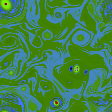
FIG. 1.: A snapshot of the vorticity field. Colors are coded according to the intensity of the vorticity field from the minima of ${\omega}$ (black) to the maxima (clear yellow,white). DNS have been performed by a standard dealiased pseudo-spectral algorithm, over a double periodic square domain of size $L=2\pi$, at resolution $512^{2}$ and $1024^{2}$. As customary enstrophy is dissipated at small scales with an hyper-viscosity of order $4$, while energy is removed at large scales, to avoid piling up on the smallest mode, using different drags (see table). We considered a Gaussian, white-in-time large-scale forcing restricted on wave numbers, $4<|k_{f}|\leq 6$.

II Two dimensional turbulence

As far as the inertial range of scales for the enstrophy cascade of two-dimensional turbulence is concerned, previous experimental, theoretical and numerical studies have shown that the statistics is strongly influenced by large-scale phenomena. Indeed more than smooth spectra $E(k)\sim k^{-\alpha}$ with $\alpha>3$, depending on the characteristics of the forcing and of the large-scale dissipation, have been reported [7, 8, 9]. Recently, new results have clarified the problem in the special case of the large scale energy sink given by a linear (Eckman) friction [8, 10]. We recall that the presence of an energy sink at large scales is conceptually justified by the necessity of avoiding the pile up of energy on the gravest mode as a result of the inverse energy cascade [4] and it is physically motivated in terms of the friction to which a fluid is subjected in the Eckman layer [18, 19].
The strong influence of large-scale phenomena in the whole enstrophy cascade range is believed to be a consequence of non local interactions (in Fourier space). Another property associated to the enstrophy cascade is the velocity field smoothness. The aim of this paper is to discuss a new set of observable suitable to highlight the statistics of all those fluctuations which appear as a sub-leading contribution to the smooth differentiable behavior, $u(x+r)-u(x)\sim r$.
Let us now briefly fix the notation. In terms of the scalar vorticity $\omega={\bf\nabla}\times{\mbox{\boldmath$u$}}$, the equation of motion can be written as

$$\partial_{t}\omega+\mbox{\boldmath$u$}\cdot{\bf\nabla}\omega=\nu_{q}\Delta^{q}\omega-\beta_{\rho}\Delta^{-\rho}\omega+F,$$ (2)

where $\nu_{q}$ and $\beta_{\rho}$ ($q,\rho\geq 0$) are the coefficients of the generalized dissipations, namely the hyper-dissipative and the hypo-friction terms respectively. The former removes enstrophy at small scales and the latter removes energy at large scales. $F$ is the vorticity source term acting at large scales. In Fig. 1, we show a typical snapshot of the vorticity field obtained by direct numerical simulation of Eq. (2). As one can see the vorticity field is characterized by filamental structure over a wide range of scales.
According to the classical prediction [3], the velocity field should exhibit a Batchelor-Kraichnan spectrum, $E(k)\sim k^{-3}(\ln(k))^{-1/3}$. The dimensional estimate is observed in a bunch of numerical and experimental measurements [20, 21]. However, in the literature there are reported numerous situations [7, 8, 9, 10] where different velocity spectra have been measured : $E(k)\sim k^{-\alpha}\,$, with the exponent $\alpha$ larger than $3$ and dependent on the forcing and drag mechanisms. In the case of linear friction, ($\rho=0$), it is known that vorticity statistics is intermittent. In such a case, it has been recently clarified [8, 10] that, at scales small enough, vorticity behaves as a passive scalar. In addition, the dependency of the spectrum slope on the linear-friction coefficient has been understood [8, 10]. Except for the situation with a large-scale linear friction, there is no general theory for the scaling properties of $2D$ turbulent flows in the presence of different large-scale drag mechanisms (see also [22]).
Let us therefore present the way we analyzed 2D turbulent flows with general large-scale physics and the related results on their statistics.

III Inverse and direct statistics for smooth signals

In this section we introduce the inverse statistics and the second difference structure functions. We start applying them to the analysis of stochastic one-dimensional signals with a given spectrum $E(k)\sim k^{-\alpha}$. For the sake of simplicity we limit our discussion to signals with $3\leq\alpha<5$, for which we are able to establish some exact results. To be more precise, we consider smooth random signals built as follows

$$s(x)=\sum_{k}{\mbox{$\hat{s}$}}(k)e^{i(kx+\theta_{k})}\,,$$ (3)

where $|{\mbox{$\hat{s}$}}(k)|^{2}\sim k^{-\alpha}$ and $\theta_{k}$ are random phases, uniformly distributed in $[0,2\pi)$. When $3\leq\alpha<5$ the signal is smooth but only one time differentiable. Hence, moments of its differences over any increment $r$ always possess a differentiable scaling (1), while moments of order $p\leq-1$ do not exist.

A Inverse statistics

For a generic smooth one-dimensional signal $s(x)$, looking at inverse statistics consists in measuring moments of the distance, $r(\delta s)$, necessary to observe in the signal a double exit (forward and backward) through a barrier $\delta s$.

FIG. 2.: A pictorial representation of the exit-distance method. $X_{i}$ and $X_{j}$ are two points picked at random and $r_{i}$ and $r_{j}$ are the corresponding exit distance from the barrier $\delta s$.

We fix a value for the signal fluctuation, $\delta s$, then we pick at random a reference point $x_{0}$ and measure the first forward ($|s(x_{0}+r_{f})-s(x_{0})|\geq\delta s$) and backward ($|s(x_{0}-r_{b})-s(x_{0})|\geq\delta s$) exit from the barrier, $r(\delta s)$. Then we put $r(x_{0},\delta s)=r_{b}+r_{f}$. See Fig. 2 for a pictorial view of the method. Repeating the observations for many point $x_{0}$ and for different barrier heights, we can define the inverse structure functions [12] as

$$T^{(p)}(\delta s)=\langle r^{p}(\delta s)\rangle\sim\delta s^{\chi(p)}\,,$$ (4)

where the average is taken with respect to the random choice of the point $x_{0}$ [23]. For the case of simple signals such as (3), a rigorous estimate of the scaling exponents of inverse statistics moments can be derived as follows. If the signal spectrum is $E(k)\sim k^{-\alpha}$ with $3\leq\alpha\,<\,5$, we can write the signal increment as

$$s(x+r)-s(x)\sim\frac{ds(x)}{dx}\,r+c(x)\,r^{h}\,.$$ (5)

Here we have only kept the two most important scaling behaviors: $O(r)$ because of the differentiability and $O(r^{h})$ from the spectrum exponent. The scaling exponent $1\leq h<2$ is related to the spectrum slope by the dimensional relation $\alpha=1+2h$, while $c(x)$ is a continuous function of $x$. By studying the exit event, in the limit of a small barrier height, we may observe two different kinds of event. The first, with probability one, is the differentiable scaling $r(\delta s)\sim\delta s$. The second, observed at those points where the first derivative vanishes, is the subleading behavior, $O(r^{h})$, in (5).
One may estimate the probability of this second situation as follows. With $3\leq\alpha<5$ the first derivative is a self-affine signal with Hölder exponent $\xi=(h-1)<1$, which vanishes on a fractal set of dimension $D=1-\xi=2-h$. Therefore, the probability to see the sub-leading term $O(r^{h})$ dominating the exit event in (5) is given by the probability to pick at random a point on a fractal set of dimension $D$, i.e.,

$$P(r\sim(\delta s)^{1/h})\sim r^{1-D}=(\delta s)^{1-1/h}.$$ (6)

Taking into account both events, we end with the following bifractal prediction for inverse statistics moments :

$$T^{(p)}(\delta s)\sim(\delta s)^{\chi_{\rm bf}(p)},\;\chi_{\rm bf}(p)=\min\!\left(p,\frac{p}{h}+1-\frac{1}{h}\right).$$ (7)

From (7), we conclude that laminar differentiable fluctuations influence the inverse statistics only up to moments of order $p=1$; for larger $p$, the PDF is dominated by the sub-dominant behavior, $(s(x+r)-s(x))\sim r^{h}$. In other words, the extrema of the signal play the role of singularities for the inverse statistics : close to the extrema, events with much longer exit distances are observed when $\delta s\rightarrow 0$. For one-dimensional signals as (3) the prediction is verified with high accuracy (see Fig. 3).
In the general multiaffine case, signal increments scale as $\delta_{r}s(x)\sim r^{h(x)}$ with probability $P_{r}(h)\sim r^{\,1-D(h)}$, where the function $D(h)$ can be interpreted as the fractal dimension of the set where the Hölder exponent $h$ is observed [24].
For such a signal, it is possible to obtain [12, 13] a link between the inverse statistics exponents, $\chi(p)$, and the fractal dimension, $D(h)$:

$$\chi(p)=\min_{h}\left({{p+1-D(h)}\over h}\right)\;.$$ (8)

In the case of the smooth signal (3), one can see that (8) coincides with the bifractal prediction (7), as soon as we write $D(h)=2-h$ for $h\equiv(1,(\alpha-1)/2)$.

FIG. 3.: Scaling exponents $\chi(p)$ for the $1D$ signal (3) with $\alpha=4$. The solid line gives the bifractal behavior. Moments have been computed using $10^{3}$ realizations of the signal (3) with $2^{17}$ modes; for each realization $2^{12}$ starting points, $x_{0}$, have been taken at random.

B Second Difference structure functions

Another way to eliminate the trivial differential scaling and extract some statistical information from smooth signals has been suggested in [17]. The basic idea is to consider moments of the second difference $\Delta_{r}s\equiv(s(x+r)+s(x-r)-2\,s(x))$, so that the differentiable contribution, $\delta_{r}s\propto r$, is automatically eliminated. For the signals under investigation, we have that at the leading order $\Delta_{r}s\sim r^{h}$ with $1\leq h<2$, and moments behave as

$$S^{(p)}_{SD}(r)\equiv\langle|\Delta_{r}s|^{p}\rangle\sim r^{z_{p}}.$$ (9)

In the monofractal case (globally self-similar signals), one expects $z_{p}=ph$. The analysis done for the same stochastic $1D$ signal of (3) with $h=1.5$, confirms this expectation (see Fig. 4).
In the general case, i.e., when many more-than-differentiable fluctuations are present, the scaling exponents $z_{p}$ are non-trivially related to the distribution of the $h$ exponents. The difficulty to give a multifractal prediction for $\Delta_{r}s$ increments stems from the fact that it is a three-point quantity, depending on the simultaneous fluctuations between ($x$, $x-r$) and ($x$, $x+r$). Therefore, to draw the multifractal picture, we would need in addition a complete control of the spatial correlations. Something which is in principle feasible [25, 26] but which goes beyond the aim of this paper.

FIG. 4.: Scaling exponent for the $1D$ signal (3) with the same parameters as in Fig. 3, the straight line shows the expected behavior $z_{p}=hp$ with $h=1.5$. The inset shows the local slope for $p=4$.

IV Spatial statistics in $2D$ smooth velocity fields

Let us now analyse the inverse and second difference statistics of the two dimensional velocity field obtained by DNS of the Navier-Stokes equation (2). We performed four different sets of numerical experiments, with periodic boundary conditions on a spatial grid of $1024^{2}$ collocation points. In all of them, we considered a Gaussian forcing, $\delta$-correlated in time, with support in a restricted band of wave numbers $4<k_{f}\leq 6$.

FIG. 5.: Log-log plot of the velocity spectra for two different drag coefficients with the Eckman linear friction, run B (middle) and run C (bottom), and with a hypodiffusive friction, run D (top). Straight-lines correspond to the best fit power laws, $k^{-3.38}$, $k^{-3.74}$ and $k^{-3.26}$ respectively. Run A is not shown because it is almost indistinguishable from run D.

In three out of four simulations, we used Eckman linear friction, i.e. $\rho=0$ in (2) with different coefficients (simulations A,B,C, in the following). In the fourth run, we used a hypo-diffusive term at large scales, $\rho=2$, (referred as case D in what follows). Table 1 is a summary of the DNS parameters, together with the best-fit spectrum exponent $\alpha$ for all runs.
In Fig. 5 we show the averaged velocity spectrum for run B,C and D (run A gives a slope almost coincident with that of run D). By comparing them, it is evident that the spectrum slope depends on both the drag coefficient (runs A,B and C) and on the drag mechanism (run D).
Evidently, we are in presence of large-scales effects which somehow affects small scales velocity fluctuations. Let us try to quantify this statement by using the inverse statistics analysis. First we compare the inverse structure functions measured on several snapshots of the DNS, with those obtained after randomization of all velocity phases on the same frames. The rationale for this test is to investigate the importance of correlations between fluctuations at different wave-numbers and therefore the “information” content brought by coherent structures in 2D turbulent flows.
If we look at a one-dimensional cut of the velocity field, before and after phases randomization, it is rather difficult to distinguish the original DNS field from that-one with randomized phases. This is due to the steepness of the spectrum, i.e., only few modes dominate the real-space configuration. Despite the apparent similarity big differences arise when looking at inverse moments.
Because of the limited numerical resolution, the only quantitative statements one can give are for relative scaling properties. Therefore, we measure scaling laws of the inverse statistics by plotting all moments $T^{(p)}(\delta u)$ versus a reference one, say $T^{(2)}(\delta u)$. This is the same technique called ESS [27], fruitfully applied in the analysis of $3D$ turbulent data with the aim of re-absorbing some finite size effects and extracting scaling information also at moderate resolution. Therefore, we concentrate on the following relative scaling properties :

$$T^{(p)}(\delta u)\propto(\,T^{(2)}(\delta u)\,)^{\chi(p)/\chi(2)}\,.$$

In Figs. 6 we summarize our findings. Inverse moment exponents, $\chi(p)/\chi(2)$, measured on the turbulent fields with randomized phases follow the bifractal prediction (7), with the value of $h$ extracted from the spectrum (see Table 1). Conversely, the longitudinal and transversal inverse-statistics moments without phases randomization show anomalous scaling laws, which deviate from the bifractal law given in (7). In Figs. 6, we show the curve $\chi(p)/\chi(2)$ for both randomized and non-randomized transversal exit moments for run C and D. For $p<1$, the statistics of the randomized data and that of the turbulent data almost coincide being those moments (with $0<p<1$) dominated by the laminar fluctuations $u(x+r)-u(x)\sim r$. To better appreciate differences in the scaling curves, we show in the inset of Figs. 6 the local slopes of $T^{(4)}(\delta u)$ versus $T^{(2)}(\delta u)$, for the randomized and non randomized data.
The following scenario can be drawn. Randomized data follow the bifractal prediction, while the non randomized ones are definitely different and display anomalous scaling. Moreover, the anomalous scaling is present for all choices of the drag mechanism.

FIG. 6.: $\chi(p)/\chi(2)$ for exit moments obtained in run C (top) and D (bottom) ($\circ$), compared with the same data after phases randomization ($\times$). In both figures, the solid line corresponds to the bifractal prediction. The values of $h$ used for the theoretical prediction are obtained from the spectrum scaling exponents (see Table 1), namely $h=1.38$ (run C) and $h=1.13$ (run D). Errors on scaling exponents have been computed according to the fluctuations of the local slopes. In each inset, it is shown the local slope of $T^{(4)}(\delta u)$ versus $T^{(2)}(\delta u)$ for the true signal ($\circ$) and the randomized one ($\times$).

For Second Difference statistics analogous results have been found, that is a monofractal behavior for the randomized field and an anomalous behavior for the turbulent one. In Figs. 7 we show the scaling exponents $z_{p}$ for run (C) and run (D). Longitudinal and transversal components, within the errors, coincide. The SD analysis confirms that the statistics of laminar events for the $2D$ turbulent velocity field displays a complex, multifractal structure.
Concerning the case of run C, i.e., with linear friction, it is interesting to compare the results of the Second Difference moments with some recent analytical results [28]. In [28], it is argued that in presence of linear Eckman friction, the second and third order (standard) structure functions behave as $S_{2}(r)=\langle\delta u^{2}(r)\rangle\sim ar^{2}+br^{2+(\alpha-3)}$ and $S_{3}(r)=\langle(\delta u(r))^{3}\rangle\sim dr^{3}+er^{\alpha}$, being $\alpha>3$ the spectrum slope, and $a,b,d,e$ some constants. From these results, it is easy to extract the exponents of the SD moments, i.e., $z_{2}=\alpha-1$ and $z_{3}=\alpha$. Actually our data give slightly larger values. Such discrepancies may be due to strong finite Reynolds effects which, in $2D$, are particularly severe due to the interplay between inverse cascade and friction in the low $k$ region of the spectrum.

FIG. 7.: (top) Second Difference exponents, $z_{p}$, for moments obtained in run (C) ($\circ$) and after randomization ($\times$); (bottom) the same but for run D. The straight lines correspond to the monofractal behaviour $z_{p}=\tilde{h}p$ with $\tilde{h}=1.55$ (run C) and $\tilde{h}=1.20$ (run D).

V Temporal statistics

As it is well known, in $3D$ turbulence we can recast the temporal behavior of the velocity field into the spatial domain via the Taylor hypothesis (frozen turbulence hypothesis): the effect of large scales is just that of a uniform sweeping which does not modify the small scale structures and their energy content. In $2D$ the absence of a time hierarchy rules out such a possibility [3, 21]. This is also evident by looking at snapshots from numerical simulations, which show that the time evolution of the dynamics is dominated by stable, long-lived structures (see Fig. 1). For such a reason it is non trivial to predict the velocity temporal statistics collected in a fixed spatial location.
We performed a DNS of (2) taking as a large-scale forcing a function $F$ of constant amplitude at some characteristic wave-numbers $4<|k_{f}|\leq 6$ and time-independent. We performed a long time integration of the $2D$ N-S equations, at resolution $512^{2}$ and collected statistics for hundreds large eddy turn over times, estimated as $t_{eddy}\approx 1/{\omega}_{rms}$ (details on the numerical simulation can be found in [29]). Once the system reached a stationary state, we started to collect the time evolution of the velocity fields at some specific spatial locations with a sampling time $\tau_{samp}\sim 2.5\cdot 10^{-2}t_{eddy}$.

FIG. 8.: (top) Time recording of the x-component of the velocity field of the $p_{in}$ probe (dotted line) and the $p_{out}$ probe (solid line);(bottom) log-log plot of the frequency spectra of the following signals: (a) $E_{p_{in}}(\varpi)$ of the probe near a coherent structure; (b) $E_{p_{out}}(\varpi)$ of the laminar one; (c) $E_{k_{f}}(\varpi)$ of the time evolution at a particular Fourier mode $k$, in forced wave-number band $|k_{f}|=(4;6]$.

Some observations are noteworthy. The first one concerns the ergodicity of the velocity field ${\mbox{\boldmath$u$}}({\mbox{\boldmath$x$}},t)$. Temporal signals collected at different spatial locations possess different probability distribution functions. In particular the range of variations of the local rms values $u_{rms}({\mbox{\boldmath$x$}_{0}},t)$ is so wide that we can not average time histories recorded at different points. It is difficult to say if waiting long enough one would recover, as expected, some stable ergodic properties. Certainly, with our statistics we feel confident to report results only on local averages, avoiding to mix temporal evolutions in different spatial locations.
In particular, we chose to report those describing two typical spatial situations: one, $p_{in}$, situated in the core of a vortical structure, the other, $p_{out}$, in a laminar region. This means that notwithstanding the turbulent evolution of the field, the motion of the vortices is so slow that probes almost maintain their respective “character” (in and out of a vortex) all the simulation long.
Looking at a sample of the time series recorded by the two probes, the signals seem very different and change when the probe passes from a laminar region to a vortical one (see Fig. 8 (top)). To have a better understanding, it is useful to consider the frequency spectra $E(\varpi)$ of the signals, calculated from the temporal Fourier transform of the stationary time correlation function, e.g., of $C(u_{x}(p),\tau)={\langle}\,u_{x}(p,t+\tau)\,u_{x}(p,t)\,{\rangle}$.
In Fig. 8 (bottom), we can observe the spectra of the two probes. At variance from the spatial spectra, it is not possible to extract a clear scaling behavior. One can only identifies an exponential decay, and a peak region located at the frequency $\varpi^{(L)}\approx 0.51/t_{eddy}$ (here and in the sequel “$(L)$” stands for “large scale”.) It is easy to recognize that $T^{(L)}$, defined as $T^{(L)}\equiv 1/\varpi^{(L)}$, is the typical time scale associated to the large-scale structures, either estimating it from the vorticity content of the largest structures $T^{(L)}=1/\sqrt{{\langle}{\omega}^{2}{\rangle}}$ or from their typical revolution time. In other words, Fig. 8 (bottom) tell us that in each spatial point the time evolution is governed by the typical oscillation frequency of the forced large-scale structures.
This is confirmed by the comparison of the spectra probes with the spectra built from the time correlation of the Fourier transformed velocity field $\hat{{\mbox{\boldmath$u$}}}({\mbox{\boldmath$k$}},t)$, at a given mode, ${\mbox{\boldmath$k$}}_{f}$, belonging to the forced wavenumber band. Indeed, all spectra posses a peak at frequency $\varpi^{(L)}$.
We now pass to investigate direct and inverse statistics of ${\mbox{\boldmath$u$}}(t)$. Direct structure functions behave trivially for both probes, $S_{p}(\tau)={\langle}[u({\bf x_{0}},t+\tau)-u({\bf x_{0}},t)]^{p}\sim c_{p}\,\tau^{p},\,$ where $u$ can be either one of the components $(u_{x},u_{y})$ or the velocity modulus.
It turns out that inverse temporal statistics does not posses good scaling laws. Therefore, we refrain from giving any quantitative statement while we concentrate on some qualitative properties showed by PDF’s of temporal inverse events measured at the two probes, $p_{in}$ and $p_{out}$.
In Fig. 9 we plot, for the probe $p_{in}$, various PDFs $P\left(\tau_{\delta u}/{\langle}\tau(\delta u){\rangle}\right)$, at varying $\delta u$, all re-scaled with their mean value ${\langle}\tau(\delta u){\rangle}$. First, we notice that PDFs collapse very well, indicating the absence of intermittency effects. Second, between the peak and the exponential tails at large $\tau$, each probability density function exhibits, on a wide range of scales, a power law behavior $P(\tau_{\delta u})\sim(\tau_{\delta u})^{-\gamma}$ with an estimated exponent $\gamma\approx-1$. On the other hand, PDFs measured on the probe outside the vortex, $p_{out}$, show a very different qualitative trend (inset of Fig. 9). In particular, there is not any clear power law behavior. This indicates that very large exit events become less and less probable outside the probe, something which must have to do with the absence of very smooth fluctuations in the vortex background.

FIG. 9.: Exit-time probability density functions $P(\tau_{\delta u})$ measured on the statistics of the probe $p_{in}$. The curves, calculated for different exit barriers $\delta u$, are normalized by their first moment. In the inset, the same for the probe $p_{out}$. In each figure, the straight line is the power law behavior $\tau_{\delta u}^{-1}$.

Altough qualitative, the inverse-statistics properties allow to distinguish among different temporal statistical behaviors associated to different fluid regions.

VI Conclusion

To summarize, we have studied inverse statistics moments for signals with a more than smooth spectrum, i.e., signals which are differentiable and with non-trivial stochastic sub-leading fluctuations. We have shown that statistical velocity properties of 2D turbulent flows are not simply described in terms of the spectrum slope. From the exit-distance analysis it is possible to highlight a whole spectrum of more-than-differentiable fluctuations. These, being connected with laminar events, are the strongest statistical signature of the large-scale coherence. Experiments with different methods of removing/pumping energy at large scales should be performed, to investigate the importance of large-scale structures in the inverse statistics of flows with different spectra. We have quantified laminar fluctuations also by using Second Differences, i.e., direct velocity increments subtracted of their linear differentiable behavior. We have found also in this case that more-than-differentiable fluctuations are not simply described by one single exponent.
As a final remark, we stress that inverse statistics provide a completely new statistical indicator with respect to the standard direct statistics observables. We have shown that such method is necessary in all those cases where non-trivial fluctuations are sub-leading with respect to the differentiable contributions. Obviously, the same kind of analysis here reported can be extended to other temporal signals, applying the method to a broad class of natural phenomena. As an example, we just mention possible applications in situations common to climatology or meteorology where estimating the probability of persistent velocity configurations, or of any other dynamical variable, is relevant. As a perspective, an important generalization is the investigation of multi-dimensional signals by studying the statistics of $d$-dimensional volumes between equispaced iso-surfaces.

VII Acknowledgments

We thank A. Vulpiani for his contribution in the early stage of this work. We acknowledge useful discussions with R. Benzi, G. Boffetta and G. Eyink. This work has been partially supported by the EU under the Grant No. HPRN-CT 2000-00162 “Non Ideal Turbulence” and the Grant ERB FMR XCT 98-0175 “Intermittency in Turbulent Systems”. M.C. is partially supported by the European Network ”Non Ideal Turbulence” (contract number HPRN-CT-2000-00162). We also acknowledge INFM support (Iniziativa di Calcolo Parallelo).

TABLE I.: Drag parameters $\rho,\beta_{\rho}$, spectrum slope $\alpha$, and the real space sub-leading scaling exponent, $h=(\alpha-1)/2$ for the various numerical experiments. The value of each $\alpha$ has been obtained by a best fit in the region $|{\mbox{\boldmath$k$}}|\approx(20-100)$ (see Fig. 5). By performing the fit in the region $|{\mbox{\boldmath$k$}}|\approx(15-60)$, slightly larger values of $\alpha$ are obtained. These discrepancies can be associated to the interplay between the inverse cascade of energy and the friction acting on it, which contanimates the upper part of the spectrum.

DNS label	$\rho$	$\beta_{\rho}$	$\alpha$	$h$
A	0	0.01	3.26(6)	1.13
B	0	0.10	3.38(8)	1.19
C	0	0.30	3.74(8)	1.37
D	2	14.0	3.26(6)	1.13

REFERENCES

- [1] U. Frisch, Turbulence: the Legacy of A. N. Kolmogorov, Cambridge University Press, Cambridge (1995).
- [2] A. Celani, A. Lanotte, A. Mazzino, and M. Vergassola, “Fronts in passive scalar turbulence,” Phys. Fluids 13, 1768 (2001).
- [3] R. H. Kraichnan, “Inertial range in two-dimensional turbulence,” Phys. Fluids 10, 1417 (1967); R. H. Kraichnan and D. Montgomery, “Two-dimensional turbulence,”Rep. Prog. Phys. 43, 35 (1980).
- [4] L. Smith and V. Yakhot, “Bose condensation and small-scale structure generation in a random force driven 2D turbulence,” Phys. Rev. Lett.71, 352 (1993).
- [5] J. Paret and P. Tabeling, “Intermittency in the two-dimensional inverse cascade of energy : Experimental observations,” Phys. Fluids 10, 3126 (1998).
- [6] G. Boffetta, A. Celani, and M. Vergassola, “Inverse cascade in two-dimensional turbulence: deviations from Gaussianity,” Phys. Rev. E 61, R29 (2000).
- [7] P. Santangelo, R. Benzi, and B. Legras, “The generation of vortices in high-resolution, two-dimensional decaying turbulence and the influence of initial conditions on the breaking of self-similarity,” Phys. Fluids A 1 (6), 1027 (1989).
- [8] K. Nam, E. Ott, T. M. Antonsen, Jr., and P. N. Guzdar, “Lagrangian chaos and the effect of drag on the enstrophy cascade in two-dimensional turbulence,” Phys. Rev. Lett. 84, 5134 (2000); K. Nam, T. M. Antonsen, Jr., P. N. Guzdar, and E. Ott, “k Spectrum of finite lifetime passive scalars in lagrangian chaotic fluid flows,” Phys. Rev. Lett. 83, 3426 (1999).
- [9] K. Ohkitani, “Wave number space dynamics of enstrophy cascade in a forced two-dimensional turbulence,”Phys. Fluids A 3 (6), 1598 (1991).
- [10] G. Boffetta, A. Celani, S. Musacchio, and M. Vergassola, “Intermittency in two-dimensional Eckman-Navier-Stokes turbulence”, E-print archive in nlin.CD/0111066 (2001).
- [11] M. Lesieur, Turbulence in Fluids, 2nd ed., Kluwer Ac. Publish., London (1990).
- [12] M. H. Jensen, “Multiscaling and structure functions in turbulence: an alternative approach,” Phys. Rev. Lett. 83, 76 (1999).
- [13] L. Biferale, M. Cencini, D. Vergni, and A. Vulpiani, “Exit time of turbulent signals: A way to detect the intermediate dissipative range,” Phys. Rev. E 60, R6295 (1999).
- [14] M. Abel, L. Biferale, M. Cencini, M. Falcioni, D. Vergni, and A. Vulpiani, “Exit-time approach to -entropy,” Phys. Rev. Lett. 84, 6002 (2000).
- [15] M. Abel, L. Biferale, M. Cencini, M. Falcioni, D. Vergni, and A. Vulpiani, “Exit-time and -entropy for dynamical systems, stochastic processes, and turbulence,” Physica D 147, 12 (2000).
- [16] L. Biferale, M. Cencini, A. Lanotte, D. Vergni, and A. Vulpiani, “Inverse statistics of smooth signals: the case of two dimensional turbulence,” Phys. Rev. Lett. 87 124501 (2001).
- [17] G. L. Eyink, “Exact results on stationary turbulence in : consequences of vorticity conservation,” Physica D 91, 97 (1996).
- [18] R. Salmon, Geophysical Fluid Dynamics, (Oxford University Press, NY, USA 1998).
- [19] M. Rivera and X.L. Wu, “External dissipation in driven two-dimensional turbulence,” Phys. Rev. Lett. 85, 976 (2000).
- [20] J. Paret, M.-C. Jullien, and P. Tabeling, “Vorticity statistics in the two-dimensional enstrophy cascade,” Phys. Rev. Lett. 83, 3418 (1999).
- [21] V. Borue, “Spectral exponents of enstrophy cascade in stationary two-dimensional homogeneous turbulence,”Phys. Rev. Lett. 71, 3967 (1993).
- [22] C. V. Tran and T. G. Shepherd, “Constraints on the spectral distribution of energy and enstrophy dissipation in forced two-dimensional turbulence”,(to appear in Physica D), E-print archive nlin.CD/0201002.
- [23] It can be shown that moments calculated in this way are the same as those calculated from a sequential average, i.e. “scanning” consecutively the time series and then using a suitable renormalization, see [13] for details.
- [24] G. Parisi and U. Frisch, “On the singularity structure of fully developed turbulence,” in Turbulence and predictability in geophysical flows, Proceed. Intern. School of Physics “E. Fermi”, eds. M. Ghil, G. Parisi, and R. Benzi, (1985).
- [25] J. O’Neil and C. Meneveau, “Spatial correlations in turbulence: Predictions from the multifractal formalism and comparison with experiments,” Phys. Fluids A 5, 158 (1993).
- [26] R. Benzi, L. Biferale and E. Trovatore, “Ultrametric structure of multiscale energy correlations in turbulent models,” Phys. Rev. Lett. 79, 1670 (1997).
- [27] R. Benzi, S. Ciliberto, R. Tripiccione, C. Baudet, F. Massaioli, and S. Succi, “Extended self-similarity in turbulent flows,” Phys. Rev. E 48, R29 (1993).
- [28] D. Bernard, “Influence of friction on the direct cascade of the forced turbulence”, Europhys. Lett. 50 (3), 333-339 (2000).
- [29] For sake of completeness, we recall that in this series of numerical simulations, enstrophy is dissipated by an hyper-viscosity term with , while energy is removed using an IR drag term with The resulting energy spectrum has the form , with .