Orbit bifurcations and wavefunction autocorrelations

Abstract

It was recently shown (Keating & Prado, Proc. R. Soc. Lond. A 457, 1855-1872 (2001)) that, in the semiclassical limit, the scarring of quantum eigenfunctions by classical periodic orbits in chaotic systems may be dramatically enhanced when the orbits in question undergo bifurcation. Specifically, a bifurcating orbit gives rise to a scar with an amplitude that scales as $\hbar^{\alpha}$ and a width that scales as $\hbar^{\omega}$, where $\alpha$ and $\omega$ are bifurcation-dependent scar exponents whose values are typically smaller than those ($\alpha=\omega=1/2$) associated with isolated and unstable periodic orbits. We here analyze the influence of bifurcations on the autocorrelation function of quantum eigenstates, averaged with respect to energy. It is shown that the length-scale of the correlations around a bifurcating orbit scales semiclassically as $\hbar^{1-\alpha}$, where $\alpha$ is the corresponding scar amplitude exponent. This imprint of bifurcations on quantum autocorrelations is illustrated by numerical computations for a family of perturbed cat maps.

1 Introduction

The local statistical properties of quantum eigenfunctions $\psi_{n}({\bf q})$ in classically chaotic systems are often modelled in the semiclassical limit by treating the eigenfunctions as random superpositions of plane waves (Berry 1977). This allows, for example, for value distributions and autocorrelation functions to be computed. However, it ignores contributions from the scarring of the eigenfunctions by classical periodic orbits (Heller 1984, Kaplan 1999). Understanding these contributions has been one of the central goals in quantum chaology. Our purpose here is to study the influence of bifurcating periodic orbits on the autocorrelation of eigenfunctions.

The semiclassical theory describing the scarring of wavefunctions by isolated and unstable periodic orbits was developed by Bogomolny (1988), who derived an explicit formula for the contribution from a given such orbit to $|\psi_{n}({\bf q})|^{2}$, averaged locally with respect to position and energy. Berry (1989) extended this approach to the Wigner functions associated with energy eigenstates, again averaged locally with respect to the energy (position averaging is unnecessary in this case). Berry’s formula also describes the influence of isolated and unstable periodic orbits on the autocorrelation of the eigenfunctions, because the Wigner function and the autocorrelation function $\langle\psi_{n}({\bf q+L})\psi_{n}^{*}({\bf q})\rangle$ are fourier transforms of each other (explicit formulae my be found in Li & Rouben 2001). It was shown in Keating (1991) that Bogomolny’s and Berry’s formulae are exact, rather than semiclassical approximations, for quantum cat maps.

The extension of Bogomolny’s theory to bifurcating periodic orbits was made in Keating & Prado (2001). There it was shown that orbits undergoing bifurcation give rise to scars in $|\psi_{n}({\bf q})|^{2}$ (averaged locally with respect to position and energy) with a width that scales as $\hbar^{\omega}$ and an amplitude that scales as $\hbar^{\alpha}$ when $\hbar\rightarrow 0$, where $\omega$ and $\alpha$ are bifurcation dependent scar exponents whose values are positive and less than or equal to those ($\omega=\alpha=1/2$) corresponding to isolated and unstable orbits. For most of the generic bifurcations $\omega<1/2$ and $\alpha<1/2$, and so bifurcations may be said to give rise to superscars. This mirrors the dominant influence they have previously been shown to exert on spectral fluctuation statistics (Berry et al. 1998, Berry et al. 2000).

The question we address here is how bifurcations influence the autocorrelation of the eigenfunctions. Our main result is that the length-scale of the correlations around a bifurcating orbit scale as $\hbar^{1-\alpha}$ when $\hbar\rightarrow 0$, where $\alpha$ is the scar amplitude exponent. By comparison, the random wave model predicts correlations with a length-scale of the order of the de Broglie wavelength (i.e. of the order of $\hbar$). We illustrate the influence of scarring on the quantum autocorrelation function with numerical computations for a family of nonlinearly perturbed cat maps (Basílio de Matos & Ozorio de Almeida 1995; Boasman & Keating 1995).

The bifurcation of periodic orbits is a characteristic phenomenon in systems whose phase space is mixed. It has been conjectured by Percival (1973) that the energy eigenstates of mixed systems separate semiclassically into those associated with stable islands (regular) and those associated with the chaotic sea (irregular). The random wave model has recently been extended to irregular states in mixed systems by Bäcker & Schubert (2002) (BS1 in the references). The autocorrelation of these states was investigated in this context in Bäcker & Schubert (2002) (BS2 in the references). Our results, concerning the length scale of the correlations, are expected to apply to the autocorrelation of irregular eigenstates in the vicinity of superscars.

2 Autocorrelation Formulae

Our purpose here is to derive semiclassical autocorrelation formulae for bifurcating periodic orbits which generalize those obtained by Berry (Berry 1989) (see also Li & Rouben 2001) for periodic orbits far from bifurcation.

The autocorrelation function for the eigenfunction $\psi_{n}({\bf q})$ of a given quantum Hamiltonian corresponding to an energy level $E_{n}$ is

$$c_{n}({\bf L})=\langle\psi_{n}({\bf q+L})\psi_{n}^{*}({\bf q})\rangle,$$ (1)

where $\langle\ldots\rangle$ denotes an average over position ${\bf q}$. We shall be particularly concerned with the case when the autocorrelation function is averaged over a group of eigenstates with energy levels near to $E$, that is with

$$C({\bf L},E,\varepsilon)=\sum_{n}c_{n}({\bf L})\delta_{\varepsilon}\left(E-E_{n}\right),$$ (2)

where $\delta_{\varepsilon}(x)$ is a normalized, Lorentzian-smoothed $\delta$-function of width $\varepsilon$. The right-hand side of (2) thus corresponds to a sum over eigenstates for which $E_{n}$ lies within a range of size of the order of $\varepsilon$ centred on $E$. Semiclassically, it is approximately the average of $c_{n}({\bf L})$ multiplied by $\overline{d}(E)$, the mean level density, which, for systems with two-degrees-of-freedom, is given asymptotically by

$$\overline{d}(E)\sim\frac{V(E)}{(2\pi\hbar)^{2}}$$ (3)

as $\hbar\rightarrow 0$, where

$$V(E)=\int\delta(E-H({\bf p},{\bf q}))d^{2}{\bf q}d^{2}{\bf p}$$ (4)

and $H({\bf p},{\bf q})$ is the classical Hamiltonian.

Our approach follows the one developed by Keating & Prado (2001) for the special case ${\bf L}={\bf 0}$. It is based on the identity

$$G({\bf q+L},{\bf q};E)=\sum_{n}\frac{\psi_{n}({\bf q+L})\psi^{\ast}_{n}({\bf q})}{E-E_{n}},$$ (5)

where $G$ is the Green function. This implies that

$$\sum_{n}\psi_{n}({\bf q+L})\psi^{\ast}_{n}({\bf q})\delta_{\varepsilon}\left(E-E_{n}\right)=-\frac{1}{2\pi i}\left\{G({\bf q+L},{\bf q};E+i\varepsilon)\right.\\ \left.-\left(G({\bf q},{\bf q+L};E+i\varepsilon)\right)^{\ast}\right\}.$$ (6)

For simplicity, we shall concentrate here on systems with time-reversal symmetry. In this case (6) reduces to

$$\sum_{n}\psi_{n}({\bf q+L})\psi^{\ast}_{n}({\bf q})\delta_{\varepsilon}\left(E-E_{n}\right)=-\frac{1}{\pi}\operatorname{Im}G({\bf q+L},{\bf q};E+i\varepsilon).$$ (7)

(As will become apparent, our analysis generalizes straightforwardly to non-time-reversal-symmetric systems.) The connection with classical mechanics is achieved using the semiclassical approximation to the Green function. For systems with two-degrees-of-freedom, this is

$$G({\bf q+L},{\bf q};E)\approx\frac{1}{i\hbar\sqrt{2\pi i\hbar}}\sum_{\gamma}\sqrt{\left|D_{\gamma}\right|}\exp{\left\{\frac{i}{\hbar}S_{\gamma}({\bf q+L},{\bf q};E)-\frac{i\pi}{2}\mu_{\gamma}\right\}},$$ (8)

where the sum includes all classical trajectories from ${\bf q}$ to ${\bf q+L}$ at energy $E$, $S_{\gamma}$ is the action along the trajectory labelled $\gamma$,

$$D_{\gamma}=\det{\left(\begin{array}[]{ll}\frac{\partial^{2}S_{\gamma}}{\partial{\bf q^{\prime}}\partial{\bf q}}&\frac{\partial^{2}S_{\gamma}}{\partial{\bf q^{\prime}}\partial E}\\ \frac{\partial^{2}S_{\gamma}}{\partial E\partial{\bf q}}&\frac{\partial^{2}S_{\gamma}}{\partial E^{2}}\end{array}\right)}$$ (9)

with ${\bf q^{\prime}}={\bf q+L}$, and $\mu_{\gamma}$ is the Maslov index (Gutzwiller 1990).

The autocorrelation formula we seek follows from averaging (7) with respect to ${\bf q}$. On the left-hand side this gives $C({\bf L},E,\varepsilon)$. On the right-hand side, the ${\bf q}$-average (via the stationary phase condition) semiclassically selects from the classical orbits with initial and final positions differing by ${\bf L}$ - henceforth we call such trajectories ${\bf L}$-trajectories - those for which the initial and final momenta are equal. Our main concern will be with cases when $|{\bf L}|$ vanishes in the semiclassical limit. Then the classical orbits contributing to the ${\bf q}$-average are close to periodic orbits. To first approximation one can thus find them by linearizing about the periodic orbits. Essentially, when a periodic orbit is isolated, this corresponds to expanding the action up to terms that are quadratic in the distance from it. Specifically, if ${\bf M}_{p}$ is the monodromy matrix associated with a periodic orbit $p$, then in a section transverse to the orbit, in which the coordinate is $y$ and the conjugate momentum is $p_{y}$ (we assume here two degrees of freedom, for simplicity),

$$\begin{pmatrix}y+L_{y}\\ p_{y}\end{pmatrix}={\bf M}_{p}\begin{pmatrix}y\\ p_{y}\end{pmatrix},$$ (10)

where $L_{y}$ is the component of ${\bf L}$ in the direction of the $y$-axis. For a given choice of $L_{y}$, this allows one to determine the coordinates of the associated orbit in the vicinity of $p$ which contributes to $C({\bf L},E,\varepsilon)$. Thus one may view the autocorrelation function semiclassically as a sum of contributions from the periodic orbits. The contribution from each periodic orbit is, within the linear approximation, stationary in $L_{y}$ when $p_{y}=0$ (i.e. on the periodic orbit itself), that is when $L_{y}=0$. This may be seen explicitly by expanding the action in (7) up to quadratic terms around the orbit $p$. Let $z$ be the coordinate along $p$. Here and in the subsequent analysis we assume that periodic orbit contributions to the autocorrelation function are $z$-independent (this is correct in determining the $\hbar$ dependence of these contributions when $|{\bf L}|\rightarrow 0$ as $\hbar\rightarrow 0$, because the $z$-dependence comes in only via the classical dynamics, except at self-focal points, which do not affect the leading order semiclassical asymptotics of the ${\bf q}$-average). The ${\bf q}$-average may then be computed (it is a Gaussian integral), giving the contribution from $p$ to be proportional to $\exp(i\eta_{p}L^{2}_{y}/\hbar)$, where $\eta_{p}$ is determined by ${\bf M}_{p}$. It is clear that this is stationary (i.e. centred) at $L_{y}=0$. More importantly for us, it also shows that the contribution from an isolated periodic orbit has a length-scale that is of the order of $\hbar^{\frac{1}{2}}$ (in contrast to the random wave model component, for which the length-scale is of the order of $\hbar$). This picture coincides precisely with Berry’s (Berry 1989) for Wigner functions. The question we now address is what is the length-scale of the contribution to the autocorrelation function from bifurcating (i.e. non-isolated) periodic orbits.

One might imagine that the autocorrelation formulae for bifurcating orbits could be obtained easily by expanding the action in (8) to higher order than quadratic. This is true for some of the simpler bifurcations (e.g. the codimension-one bifurcations of orbits with repetition numbers $r=1$ and $r=2$ - see the examples in Section 3), but for more complicated bifurcations it is incorrect, because for these the linearized map ${\bf M}^{r}_{p}$ is equal to the identity, which cannot be generated by the action $S({\bf q^{\prime}},{\bf q};E)$. Thus it is difficult to build into the semiclassical expression for the ${\bf qq^{\prime}}$-representation of the Green function a well-behaved description of the nonlinear dynamics which the linearized map approximates. The solution to this problem, found by Ozorio de Almeida & Hannay (1987), is to transform the Green function to a mixed position-momentum representation, and this is the approach we now take.

The method just outlined involves, first, Fourier transforming $G({\bf q^{\prime}},{\bf q};E)$ with respect to ${\bf q^{\prime}}$. This gives the Green function in the ${\bf q}$ ${\bf p^{\prime}}$-representation, $\tilde{G}({\bf p^{\prime}},{\bf q};E)$ (${\bf p^{\prime}}$ is the momentum conjugate to ${\bf q^{\prime}}$). The semiclassical approximation to $\tilde{G}$ takes the same form as (8), except that $S({\bf q^{\prime}},{\bf q};E)$ is replaced by the ${\bf q}$ ${\bf p^{\prime}}$-generating function $\tilde{S}({\bf p^{\prime}},{\bf q};E)$. $G({\bf q^{\prime}},{\bf q};E)$ may then be rewritten, semiclassically, as the Fourier transform of this expression with respect to ${\bf p^{\prime}}$. The result, for the semiclassical contribution to $G({\bf q+L},{\bf q};E)$ from classical orbits in the neighbourhood of a bifurcating periodic orbit, takes the following form.

Consider the general case of a codimension-$K$ bifurcation of a periodic orbit with repetition number $r$. As before, let $z$ be a coordinate along the orbit at bifurcation, let $y$ be a coordinate transverse to it, and let $p_{y}$ be the momentum conjugate to $y$, so that $y$ and $p_{y}$ are local surface of section coordinates. We again assume the semiclassical $\hbar$-scaling of the length-scale of the contribution from the bifurcating orbit to the autocorrelation function to be $z$-independent. Let $\Phi_{r,K}(y,p_{y},{\bf x})$ be the normal form which corresponds to the local (reduced) generating function in the neighbourhood of the bifurcation (Arnold 1978; Ozorio de Almeida 1988), where ${\bf x}=(x_{1},x_{2},\cdots,x_{K})$ are parameters controlling the unfolding of the bifurcation. Then, up to irrelevant factors, the contribution to $G({\bf q+L},{\bf q};E)$ is

$$G_{r,K}(y,L_{y};{\bf x})\propto\frac{1}{\hbar^{2}}\int\exp{\left[\frac{i}{\hbar}\Phi_{r,K}(y,p_{y},{\bf x})+\frac{i}{\hbar}p_{y}L_{y}\right]}dp_{y}$$ (11)

(as already stated, we are here interested in determining the $\hbar$-dependence of the length-scale of contributions to the autocorrelation function, and so have neglected terms in (11), such as an $\hbar$-independent factor in the integrand, which do not influence this). Note that it follows from the definition of the generating function that the stationary phase condition with respect to $p_{y}$ selects classical orbits for which the initial and final $y$-coordinates differ by $L_{y}$; that then the stationary phase condition with respect to $y$ (which gives the semiclassical contribution to the $y$-average needed to compute the autocorrelation formula) further selects from these orbits those whose initial and final momenta, $p_{y}$, are identical; and that the orbits contributing at the point where $G_{r,K}$ is stationary with respect to $L_{y}$ are those for which $p_{y}=0$.

We now follow the steps taken in Keating & Prado (2001) for the case when $L_{y}=0$: first, rescale $y$ and $p_{y}$ to remove the $1/\hbar$ factor from the dominant term (germ) of $\Phi_{r,K}$ in the exponent, and then apply a compensating rescaling of the parameters $x_{1},x_{2},\cdots,x_{K}$ to remove the $\hbar$-dependence from the other terms which do not vanish as $\hbar\rightarrow 0$. Finally, we then rescale $L_{y}$ to remove the $\hbar$-dependence of the second term in the exponent in (11). Crucially, this term only involves $p_{y}$, and so if in the initial rescalings

$$p_{y}\rightarrow\hbar^{\alpha_{r,K}}p_{y}$$ (12)

then the length scale of the corresponding contribution to the autocorrelation function is of the order of $\hbar^{1-\alpha_{r,K}}$. This is our main general result. It is important to note that $\alpha_{r,K}$ is precisely the exponent found for the scarring amplitude in Keating & Prado (2001). This then implies a sum rule for the scaling exponents of scar amplitudes and the length-scale exponents of wave function correlations reminiscent of those found in the theory of critical phenomena. It is worth emphasizing that the correlation length-scale is related to the amplitude exponent, rather than the width exponent (denoted $\omega_{r,K}$ in Keating & Prado 2001).

Values of $\alpha_{r,K}$ were computed by Keating & Prado (2001) for the generic bifurcations found in two-degree-of-freedom systems using the appropriate normal forms. For convenience, we list here the results. First, for the $r=1$ (i.e. saddle-node) bifurcations which correspond to cuspoid (i.e. corank 1) catastrophes, $\alpha_{1,K}=\frac{1}{2}$. Values of $\alpha$ for the generic bifurcations with $r>1$ and $K=1$ are listed in Table 1, and those for $r>1$ and $K=2$ in Table 2. Finally, $\alpha_{r,K}=\frac{1}{2(K+1)}$ in the general case of bifurcations of orbits for which $r\geq 2K+2$.

$r$	$2$	$3$	$\geq 4$
$\alpha_{r,1}$	$1/2$	$1/3$	$1/4$

Table 1: Values of $\alpha_{r,1}$ for the generic, codimension-1 bifurcations.

$r$	$2$	$3$	$4$	$5$	$\geq 6$
$\alpha_{r,2}$	$1/2$	$1/4$	$1/4$	$1/5$	$1/6$

Table 2: Values of $\alpha_{r,2}$ for the generic, codimension-2 bifurcations.

Note that in all cases listed above $0<\alpha\leq 1/2$, and that in most cases $\alpha<1/2$. Thus the length scale of the fringes $\hbar^{1-\alpha_{r,K}}$ is always semiclassically equal to or smaller than for non-bifurcating orbits, and in most cases is smaller. In all cases it is semiclassically larger than the de Broglie wavelength.

The rescaling of $y$ in (11) was defined in Keating & Prado (2001) by

$$y\rightarrow\hbar^{\omega_{r,K}}y,$$ (13)

where $\omega_{r,K}$ is the scar width exponent. In the case of the autocorrelation function, one must average over $y$. This leads to the amplitude of $G_{r,K}$ being proportional to $\hbar^{\alpha_{r,K}+\omega_{r,K}-2}$. We remark that the exponent of $\hbar$ in the amplitude is related to amplitude exponent $\beta$ (Berry et al. 2000) of the fluctuations in the spectral counting function associated with the bifurcation in question, because

$$\alpha_{r,K}+\omega_{r,K}-2=-(\beta_{r,K}+1)$$ (14)

(see equation (2.25) in Keating & Prado 2001).

The rescaling of $x_{n}$ in (11) was defined in Keating & Prado (2001) by

$$x_{n}\rightarrow\hbar^{\sigma_{n,r,K}}x_{n}.$$ (15)

Here, the exponents $\sigma$ describe the range of influence of the bifurcation in the different unfolding directions $x_{n}$, and their sum

$$\gamma_{r,K}=\sum_{n=1}^{K}\sigma_{n,r,K}$$ (16)

describes the $\hbar$-scaling of the $K$-dimensional ${\bf x}$-space hypervolume affected by the bifurcation.

3 Perturbed cat maps

We now illustrate some of the ideas described in the previous section by focusing on a particular example: a family of perturbed cat maps. The influence of bifurcations on the scarring of eigenfunctions was explored numerically for these systems in Keating & Prado (2001). (The influence of tangent bifurcations on localization in wavefunctions was also investigated numerically for a different family of maps by Varga et al. 1999). We focus here on eigenfunction autocorrelations.

The maps we consider are of the form

$$\left(\begin{array}[]{l}q_{n+1}\\ p_{n+1}\end{array}\right)=\left(\begin{array}[]{ll}2&1\\ 3&2\end{array}\right)\left(\begin{array}[]{l}q_{n}\\ p_{n}\end{array}\right)+\frac{\kappa S^{{}^{\prime}}_{p}(q_{n})}{4\pi^{2}}\left(\begin{array}[]{l}1\\ 2\end{array}\right)\mbox{mod 1},$$ (17)

where $S^{{}^{\prime}}_{p}(q)$ is the first derivative of a periodic function with period $1$, $\kappa$ is a parameter determining the size of the perturbation, and $q$ and $p$ are coordinates on the unit two-torus which are taken to be a position and its conjugate momentum. We will consider two cases: $S_{p}(q)=\sin{(2\pi q)}$ and $S_{p}(q)=\cos{(2\pi q)}$.

These maps are Anosov systems. In both cases, for $\kappa\leq\kappa_{\rm max}=(\sqrt{3}-1)/\sqrt{5}\approx 0.33$ they are completely hyperbolic and their orbits are conjugate to those of the map with $\kappa=0$ (i.e. there are no bifurcations). Outside this range, bifurcations occur, stable islands are created, and the dynamics becomes mixed (Berry et al. 1998, Keating & Prado 2001).

The quantization of maps like (17) was developed by Hannay & Berry (1980), when $\kappa=0$, and Basílio de Matos & Ozorio de Almeida (1995) for non-zero $\kappa$. The quantum kinematics associated with a phase space that has the topology of a two-torus restricts Planck’s constant to taking inverse integer values. The integer in question, $N$, is the dimension of the Hilbert space of admissible wavefunctions. With doubly periodic boundary conditions (see, for example, Keating et al. 1999), these wavefunctions in their position representation have support at points $q=Q/N$, where $Q$ takes integer values between 1 and $N$. They may thus be represented by $N$-vectors with complex components. The quantum dynamics is then generated by an $N\times N$ unitary matrix ${\bf U}$ whose action on the wavefunctions reduces to (17) in the classical limit; for example

$$U_{Q_{2},Q_{1}}=\frac{1}{\sqrt{iN}}\exp\left[\frac{2\pi i}{N}(Q_{1}^{2}-Q_{1}Q_{2}+Q_{2}^{2})+\frac{iN}{2\pi}\kappa\sin(2\pi Q_{1}/N+\pi\nu/2)\right].$$ (18)

where $\nu=0$ gives the sine perturbation and $\nu=1$ the cosine perturbation. This matrix plays the role of the Green function of the time-dependent Schrödinger equation for flows.

Denoting the eigenvalues of ${\bf U}$ by ${\rm e}^{i\theta_{n}}$ and the corresponding eigenfunctions by $\Psi_{n}(Q)$, we have, using the fact that the map (17) is invariant under time-reversal and hence that ${\bf U}$ is symmetric, that

$$C(L,\theta,\epsilon)=\sum^{N}_{n=1}c_{n}(L)\delta_{\varepsilon}(\theta-\theta_{n})=\delta_{L,0}+\frac{1}{N}\operatorname{Re}\sum^{N}_{Q=1}\sum^{\infty}_{k=1}U_{Q+L,Q}^{k}\exp{(-i\theta k-\varepsilon k)}$$ (19)

where

$$c_{n}(L)=\frac{1}{N}\sum_{Q=1}^{N}\Psi_{n}(Q+L)\Psi^{\ast}_{n}(Q)$$ (20)

is the eigenvector autocorrelation function and

$$\delta_{\varepsilon}(x)=\frac{1-e^{-\varepsilon}\cos{x}}{1+e^{-2\varepsilon}-2e^{-\varepsilon}\cos{x}}$$ (21)

is a periodized, Lorentzian-smoothed $\delta$-function of width $\varepsilon$ (Keating 1991). Equation (19) is the analogue for quantum maps of (7). $C(L,\theta,\epsilon)$ corresponds, approximately, to $N$ times the local $n$-average (over a range of size of the order of $\varepsilon$) of $c_{n}(L)$. For $\varepsilon$ large enough, the dominant contribution to (19) comes from the $k=1$ term in the sum on the right. We thus define

$$c(L,\theta,\epsilon)=\frac{1}{N}\sum^{N}_{Q=1}U_{Q+L,Q}\exp{(-i\theta-\varepsilon)}.$$ (22)

and, for computational purposes,

$$c_{r}(L,\theta,\epsilon)=\frac{1}{N}\operatorname{Re}\sum^{N}_{Q=1}U_{Q+L,Q}\exp{(-i\theta-\varepsilon)}.$$ (23)

We may substitute (18) directly into (22). In the semiclassical limit, as $N\rightarrow\infty$, the $Q$-average selects regions close to stationary points of the phase of (18). When $L=0$ these stationary points coincide with the positions of the fixed points of the classical map (17); otherwise the stationary solutions correspond to $l$-trajectories - in this case classical trajectories with initial and final coordinates separated by $l=L/N$ and with initial and final momenta equal to each other. These satisfy

$$q_{j}(l)=\frac{1}{2}\left(j-l-\frac{\kappa}{2\pi}\cos{(2\pi q_{j}+\nu\frac{\pi}{2}})\right)$$ (24)

for integers $j$ such that $0\leq q_{j}(l)<1$ (see, for example, Boasman & Keating 1995). When $l\rightarrow 0$ (which is the most important regime, given that we wish to focus on correlation length-scales that vanish semiclassically) the $l$-trajectories obviously lie close to fixed points of the map.

Expanding the phase of (18) around ${q}_{j}$ up to cubic terms gives

$$U_{Q+L,Q}\approx\frac{1}{\sqrt{iN}}\exp\left[2\pi iNS_{j}+\pi iN\left(2-\kappa\sin\left(2\pi q_{j}+\nu\frac{\pi}{2}\right)\right)y^{2}\right.\\ \left.-\frac{2\pi^{2}iN}{3}\kappa\cos\left(2\pi q_{j}+\nu\frac{\pi}{2}\right)y^{3}\right],$$ (25)

where

$$y=q-q_{j}(l)$$ (26)

and $2\pi NS_{j}$ denotes the phase evaluated at $q_{j}(l)$. Provided that $2-\kappa\sin(2\pi q_{j}+\nu\pi/2)\neq 0$, this approximation is dominated by the quadratic term in the exponent when $y$ is small. It thus describes complex-Gaussian fringes around the classical $l$-trajectories with a length-scale (in terms of $y$) of the order of $N^{-1/2}$.

As discussed in Section 2, the centres of the peaks of the autocorrelation function are given by contributing $l$-trajectories that start at $q$, end at $q+l$, and satisfy $p^{\prime}=p=0$ in the first iterate of the map (17). From (17), the peak centres are thus solutions of

$$l=q+\frac{\kappa}{2\pi}\cos{(2\pi q+\nu\pi/2)}-n$$ (27)

and

$$3q+\frac{\kappa}{\pi}\cos{(2\pi q+\nu\pi/2)}-m=0$$ (28)

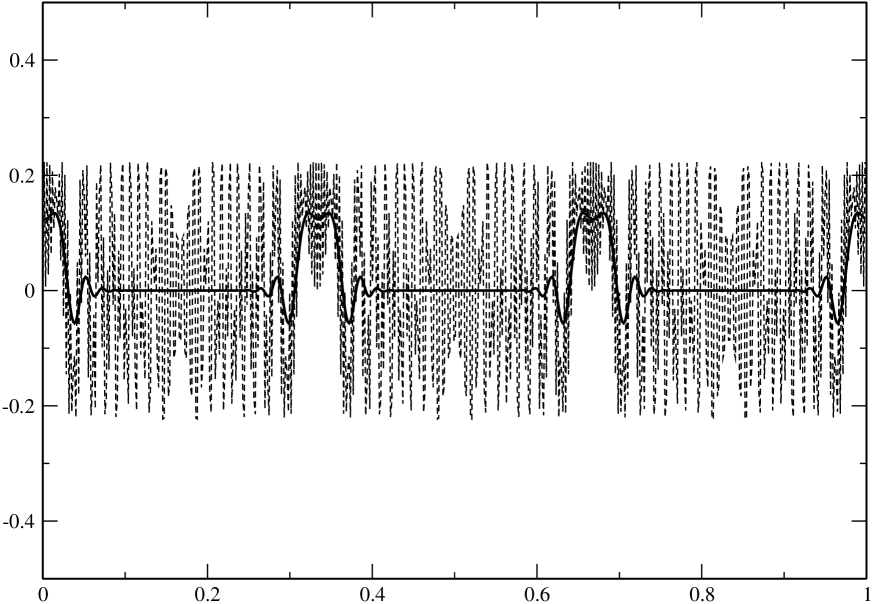
Figure 1: $c_{r}(L,\theta,\epsilon)$ plotted as a function of $l=L/N$ with $N=597$, $\kappa=0.0$ (i.e. no perturbation), $\epsilon=1.5$ and $\theta=\pi/4$ (dashed line). The bold line represents a convolution of the data with a normalized Gaussian of width 0.007.

where $m$ and $n$ are integers. For the linear mapping, when $\kappa=0$, the peaks are centred at $l=q=m/3$ with $m=0,1,2$. These peaks may be seen in Figure 1, where the dashed line represents an evaluation of (23) and the bold line a convolution of the data with a normalized Gaussian of width 0.007.

For $\kappa>0$ the peak location equations, (27) and (28), can be solved numerically. As $\kappa$ increases bifurcations of periodic orbits take place. It is important at this stage to distinguish between the birth of new periodic orbits as the perturbation parameter $\kappa$ is varied (the usual bifurcation) and the birth of new $l$-trajectories as $l$ varies (a process which we call an $l$-caustic). As $l\rightarrow 0$, the $l$-trajectories are close to periodic orbits. $l$-caustics coincide with periodic orbit bifurcations in the limit.

Our main purpose now is to illustrate quantitatively the influence of bifurcating periodic orbits on the autocorrelation function. We shall study in detail two bifurcations: one a first order (tangent) bifurcation, and the other a second order bifurcation. In order to do so, we will treat separately the sine and cosine perturbations.

3.1 Sine perturbation $\nu=0$

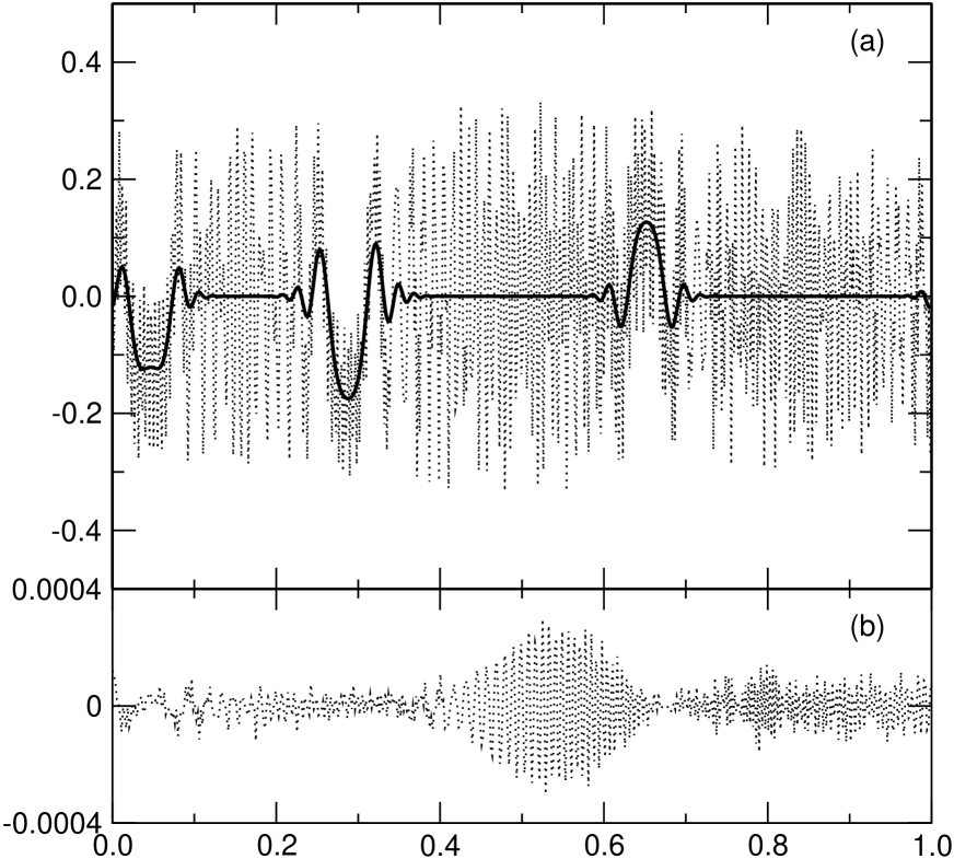
Figure 2: (a) $c_{r}(L,\theta,\epsilon)$ plotted as a function of $l=L/N$ for the sine perturbation with $N=597$, $\kappa=1.0$, $\epsilon=1.5$ and $\theta=\pi/4$ (dashed line). The bold line represents a convolution of the data with a normalized Gaussian of width 0.007. In (b) the difference between the exact expression (23) and the semiclassical approximation (30) is plotted.

For $\kappa>0$, the positions of the peaks in the autocorrelation function deviate from those ($0$, $1/3$ and $2/3$) of the unperturbed map ($\kappa=0$). The real part of the autocorrelation function for $\kappa=1$ is shown in Figure 2 (a). The peak close to $l=0$ comes from the contribution of the period-1 fixed point $j=0$ in (24). Using a stationary phase approximation with respect to $L$ in (25) gives the position of the peak to be

$$l\approx\frac{\kappa}{\pi}\frac{\cos{(2\pi q_{0}(0))}}{3-\kappa\sin(2\pi q_{0}(0))}{\mbox{ mod 1}}$$ (29)

in the limit as $l\rightarrow 0$. For $\kappa\sin(2\pi q_{j}))<2$, the second order term in the Taylor expansion (25) dominates and the semiclassical formula for the autocorrelation function is simply

$$c_{r}(L,\theta,\epsilon)\approx\sum^{1}_{j=0}\exp{(-\varepsilon)}\frac{\cos{(2\pi NS_{j}-\theta+(\zeta-1)\pi/4)}}{\sqrt{|2-\kappa\sin{(2\pi q_{j}(l)})|}}$$ (30)

where $\zeta={\mbox{sign}}(2-\kappa\sin{(2\pi q_{j}(l))})$ and

$$S_{j}=\frac{3l^{2}}{4}+j\frac{l}{2}-j\frac{1}{4}+\frac{\kappa}{4\pi^{2}}\sin{(2\pi q_{j}(l))}+\frac{\kappa^{2}}{16\pi^{2}}\cos^{2}{(2\pi q_{j}(l))}.$$ (31)

In figure 2 (b) we plot the difference between the exact expression (23) and the semiclassical approximation (30).

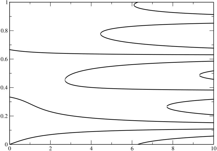
Figure 3: Predicted peak-centres in the autocorrelation function due to $l$-trajectories, computed by solving (27) and (28), for the sine perturbation.

For larger $\kappa$, keeping terms only up to second order in the approximation (25) fails in two ways. First, $2-\kappa\sin(2\pi q_{j}(l))$ vanishes for some values of $l$ and higher terms of the expansion of the action need to be taken into account. It is clear in Figure 3, where the predicted peak-centres (obtained by solving (27) and (28)) are plotted, that for $\kappa$ around $3.0$ new $l$-trajectories contribute to the autocorrelation with a peak around $l=0.5$. Although these $l$-caustics are an additional complication, they are in fact unimportant if the object is to compute the contribution of bifurcating periodic orbits which takes place for $l$ around zero (recall that this is the region that is semiclassically interesting for correlation length-scales that vanish with $\hbar$).

Second, when $l\rightarrow 0$, $2-\kappa\sin(2\pi q_{j}(0))=0$ at periodic orbit bifurcations. Then again the quadratic term in (25) vanishes, and the fringe structure comes from the cubic term. It thus has a $y$-length-scale of the order of $N^{-1/3}$. In the language of Section 2, this corresponds to a codimension-one bifurcation of a periodic orbit with $r=1$ (a tangent bifurcation). The $j=0$ and $j=1$ terms each correspond to a single unstable fixed point if the condition $2-\kappa\sin(2\pi q_{j}(l))\neq 0$ is satisfied. Note that at both $l$-caustics and tangent bifucations, the semiclassical asymptotics is determined by the cubic term in the expansion of the action; hence both contributions are of the same order in $\hbar$.

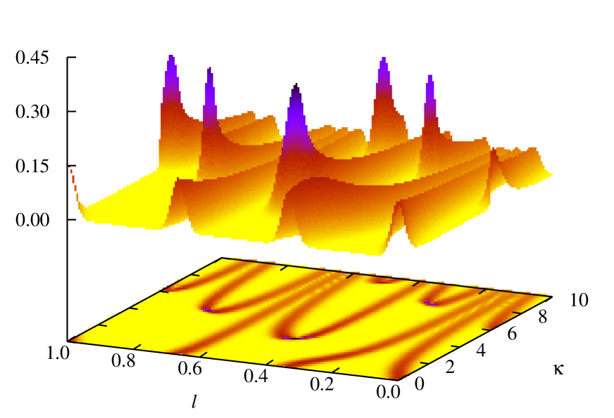
Figure 4: The absolute value of the convolution of the autocorrelation function (22) with a normalized Gaussian of width 0.01, plotted as a function of $\kappa$ and $l=L/N$ for the sine perturbation with $N=597$, $\epsilon=1.5$ and $\theta=\pi/4$. A projection is shown underneath. Compare the positions of the ridges with the theoretical curves shown in Figure 3. Note also the enhanced amplitude near the bifurcation and the $l$-caustics.

Figure 4 provides a panorama of the situation. Here, the absolute value of the Gaussian smoothed autocorrelation function $c$ is plotted. The result should be compared with the predicted peak-centres shown in Figure 3. The peak coming from the bifurcating periodic orbits is around $\kappa=6$ and $l=0$. The other similar peaks are all associated with the $l$-caustics. It is clear that their amplitudes are much larger than those of the peaks associated with isolated $l$-trajectories.

For the sine perturbation, the first bifurcation occurs when $\kappa=\kappa^{*}=5.943388$. At this parameter value, two new degenerate solutions of (24) appear for both $j=0$ and $j=1$, corresponding in each case to the birth of a pair of fixed points, one stable and the other unstable. For $l=0$ the contributions of these bifurcating orbits when $\kappa=\kappa^{\ast}$ are:

$$c_{r}(0,\theta,\epsilon)\approx\sum^{1}_{j=0}\frac{N^{1/6}}{\Gamma(2/3)}\left(\frac{4\pi}{9\kappa^{\ast}}\right)^{1/3}\exp{(-\varepsilon)}\frac{\cos{(2\pi iN{\overline{S}}_{j}-\theta-\pi/4)}}{|\cos{(2\pi{\overline{q}}_{j})}|^{1/3}}$$ (32)

where ${\overline{S}}_{j}=(S({q_{+}}_{j})+S({q_{-}}_{j}))/2$ is the average of the actions of the two bifurcating fixed points at ${q_{+}}_{j}$ and ${q_{-}}_{j}$. More generally, the semiclassical contributions of the real orbits plus the complex orbits to the autocorrelation function give:

$$c_{r}(L,\theta,\epsilon)\approx\sum^{1}_{j=0}\exp{(-\varepsilon)}\frac{\cos{(2\pi NS_{j}-\theta+(\sigma-1)\pi/4)}}{\sqrt{|2-\kappa\sin{(2\pi q_{j}(l)})|}}+\\ \operatorname{Re}{\sum^{1}_{j=0}\exp{({-\varepsilon})}N^{1/6}\frac{{\mbox{Ai}}\left[-(2\pi N|\alpha|)^{2/3}\right]}{2\pi|\alpha|^{1/3}}\sigma^{2}\exp{(2\pi iN{\overline{S}}_{j}-i\theta-i\pi/4)}}.$$ (33)

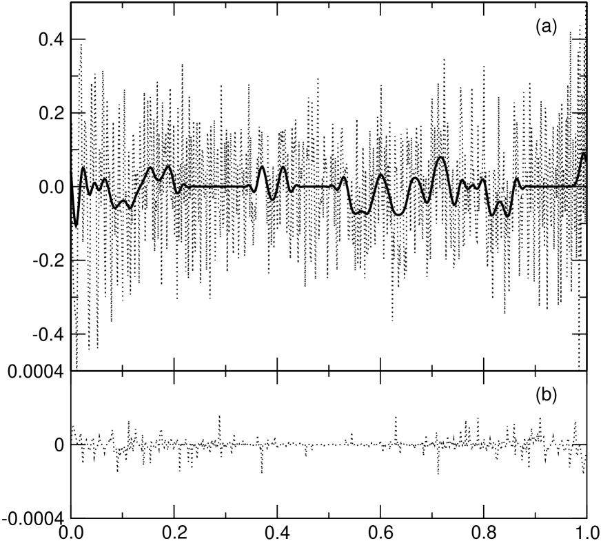
Figure 5: (a) $c_{r}(L,\theta,\epsilon)$ plotted as a function of $l=L/N$ for the sine perturbation with $N=597$, $\kappa=5.943388$, $\epsilon=1.5$, $\theta=\pi/4$ and $\theta=\pi/4$ (dashed line). The bold line represents a convolution of the data with a normalized Gaussian of width 0.007. In (b) the difference between the exact expression (23) and the semiclassical approximation (33) is plotted.

Here $\sigma=(q_{+}-q_{-})/2$ and $|\alpha|=3|\Delta S|/(2\sigma^{3})$, where $\Delta S=(S(q_{+})-S(q_{-}))/2$. Figure 5 (a) shows the autocorrelation function for $\kappa=\kappa^{\ast}$. In Figure 5 (b) the deviation of the semiclassical approximation (33) from the exact expression (23) is plotted.

3.2 Cosine perturbation $\nu=1$

Setting $\nu=1$ in (18) and the following equations allows us now to discuss a second order bifurcation. (Such bifurcations occur for the second iterate of the map with the sine perturbation, and so quantum mechanically influence $U^{2}(Q,Q)$. In the case of the cosine perturbation, they occur for fixed points of the map, and so influence $U(Q,Q)$. This makes them easier to study numerically (Mende (1999).)

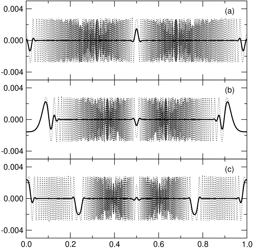
Figure 6: $\sum_{n}|\Psi_{n}(Q)|^{2}\delta_{\varepsilon}(\theta-\theta_{n})-1$ with $\varepsilon=2.2$, $\theta=\pi/4$ and $N=1597$ (dashed line) for the cosine perturbation. Also shown is a convolution of the data with a normalized Gaussian of width 0.007 (bold line). In (a) $\kappa=1.0$ and there is only one real unstable fixed point (the central fixed point) at the origin; in (b) $\kappa=2.0$, which is the parameter value at which the second order bifurcation takes place; in (c) $\kappa=3.0$, and there are two new real unstable fixed points at $q\approx 0.23$ and $q\approx 0.77$ in addition to the central fixed point, which is still located at the origin, but now is stable.

As the order of the first non-vanishing derivative of the action $S_{p}(q)$ determines the order of the bifurcation, one can see that there are no higher bifurcations than those of second order for this perturbation. For $j=0$, $q=0$ and $\kappa=2$, a bifurcation of order two occurs. For $j=1$ there is no such bifurcation: in this case only tangent bifurcations occur, the first one at $\kappa\approx 9.208$ (Mende 1999). As the tangent bifurcation was discussed previously, we will concentrate on the bifurcation of order two. For this, when $\kappa<2$ there is one real unstable fixed point (called the central fixed point), while for $\kappa>2$ there are two real fixed points (satellites) in addition to the central fixed point, which is now stable. The scarring of the wavefunctions caused by this bifurcation is shown as a dashed line is Figure 6, where $\sum_{n}|\Psi_{n}(Q)|^{2}\delta_{\varepsilon}(\theta-\theta_{n})-1$ is plotted for (a) $\kappa=1$ (one real unstable fixed point ($j=0$) at $q=0$ and another real unstable fixed point ($j=1$) at $q=0.5$), (b) $\kappa=\kappa^{\ast}=2$ (where the $j=0$ fixed point bifurcates), and (c) $\kappa=3$ (three real $j=0$ fixed points - unstable satellites at $q=-0.23$ and $q=0.23$ and the central fixed point at $q=0$, which is now stable - and the unstable $j=1$ fixed point at $q=0.5$). A convolution of the data with a normalized Gaussian of width 0.02 is also shown (bold line).

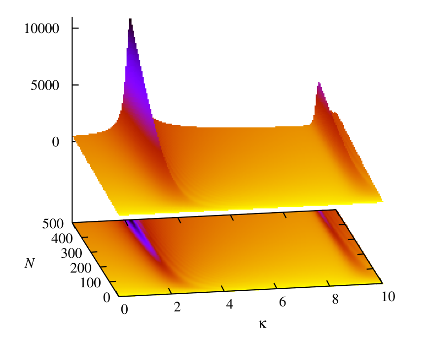
Figure 7: $|{\rm Tr}U(\kappa,N)|^{2}$ plotted as a function of $\kappa$ and $N$ for the cosine perturbation. Note the two ridges: one due to the tangent bifurcation (at $\kappa\approx 9.208$) and the other due to the second order bifurcation (at $\kappa=2$). A projection of the data is shown underneath.

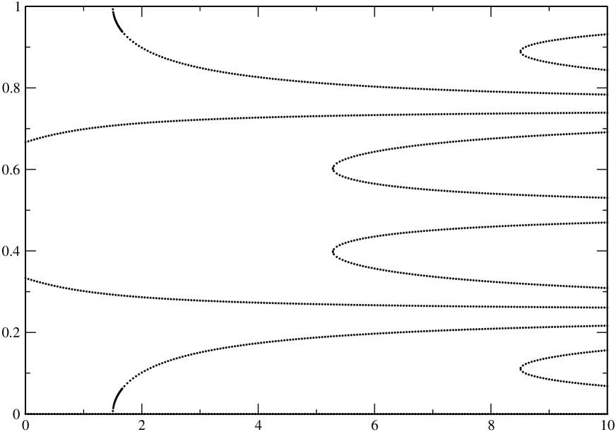
Figure 8: Predicted peak-centres in the autocorrelation function due to $l$-trajectories, computed by solving (27) and (28), for the cosine perturbation.

In Figure 7, $|\sum_{Q=1}^{N}U(Q,Q)|^{2}=|{\rm Tr}U|^{2}$ is plotted as a function of $\kappa$ and $N$. One sees the contribution of the second order bifurcation of the $j=0$ fixed point around $\kappa=2$ and that of the tangent bifurcation of the $j=1$ fixed point around $\kappa=9$. The amplitude associated with the second order bifurcation is clearly semiclassically larger. Similarly, the amplitude of the autocorrelation function is larger at these points (compare (34) below with (32)). The predicted positions of the peaks in the autocorrelation function (obtained by solving (27) and (28), when $\nu=1$) are shown in Figure 8. Here again, for $\kappa=0$ the peaks are centred at $l=0\equiv 1$, $l=1/3$ and $l=2/3$, as previously described. As $\kappa$ increases, these peaks deviate from their original positions, but the autocorrelation result for isolated points, the analogue of (30), is still valid. For $\kappa$ around 2, where the second order bifurcation occurs, the approximation (25) breaks down and an expansion of the phase of (18) around ${q}_{j}$ up to fourth order terms is necessary. The contribution of the bifurcating fixed point ($j=0$) when $\kappa=\kappa^{\ast}=2$ and $L=0$ is

$$c_{r}(0,\theta,\epsilon)\approx\frac{N^{1/4}}{2\sqrt{2}\Gamma(3/4)}\left(\frac{3\pi}{\kappa^{\ast}}\right)^{1/4}\exp{(-\varepsilon)}\cos{(2\pi iN{S_{0}}-\theta-\pi/4)}$$ (34)

where ${S_{0}}$ is the action of central orbit at $q=0$. More generally, for $\kappa\lesssim 9$ the semiclassical approximation to the autocorrelation function is

$$c_{r}(L,\theta,\epsilon)\approx\left\{\frac{\cos{(2\pi NS_{1}-\theta+(\zeta-1)\pi/4)}}{\sqrt{|2-\kappa\cos{(2\pi q_{1}(l))}|}}\right.\\ +\left.\operatorname{Re}{\frac{\pi}{2}N^{1/2}q_{s}(l)\left[{\mbox{J}}_{-1/4}(z)\exp{(i\sigma_{1})}+{\mbox{sign}}(2-\kappa){\mbox{J}}_{1/4}(z)\exp{(i\sigma_{2})}\right]}\right\}\exp{(-\varepsilon)}.$$ (35)

Here $q_{s}(l)$ is the distance of the satellite points from the origin, $z=\pi N\alpha q_{s}^{4}/4$, where $\alpha=4(-q_{s}^{2}+\kappa(1-\cos{(2\pi q_{s})}))/q_{s}^{4}$, $\sigma_{1}=-\theta-\pi/8+2\pi NS_{0}-\pi N\alpha q_{s}^{4}/4$, and $\sigma_{2}=-\theta+5\pi/8+2\pi NS_{0}-\pi N\alpha q_{s}^{4}/4$.

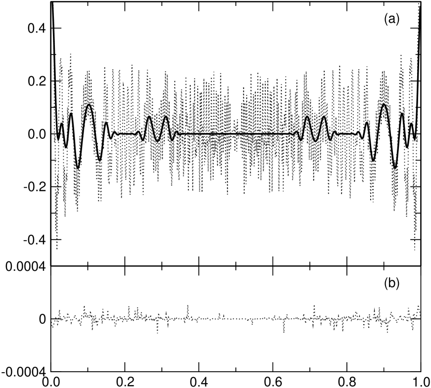
Figure 9: (a) $c_{r}(L,\theta,\epsilon)$ plotted as a function of $l=L/N$ for the cosine perturbation with $N=597$, $\kappa=2$, $\epsilon=1.5$ and $\theta=\pi/4$ (dashed line). The bold line represents a convolution of the data with a normalized Gaussian of width 0.007. In (b) the difference between the exact expression (23) and the semiclassical approximation (35) is plotted.

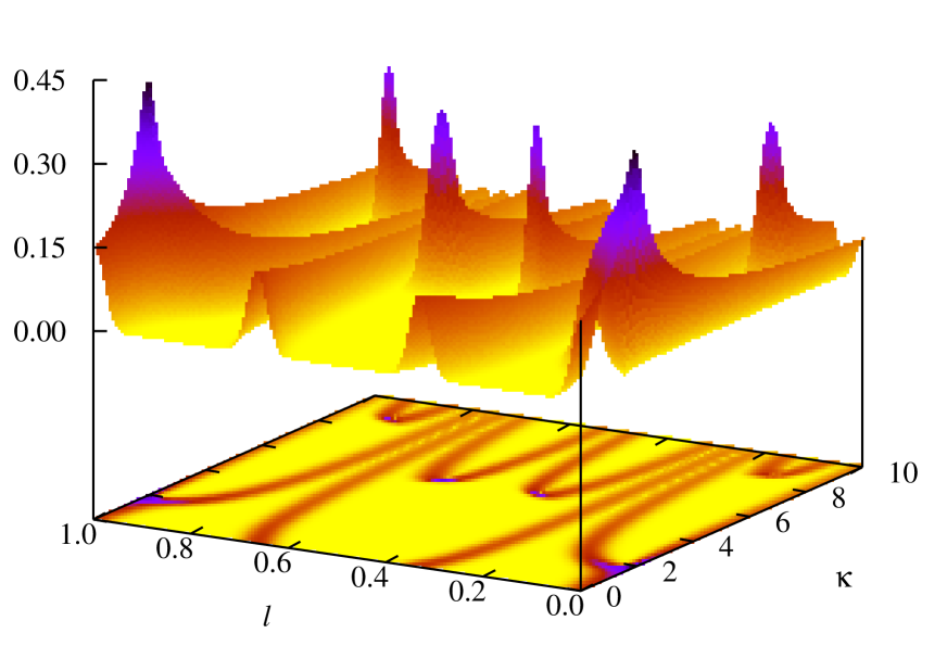
Figure 10: The absolute value of the convolution of the autocorrelation function (22) with a normalized Gaussian of width 0.01 plotted as a function of $\kappa$ and $l=L/N$ for the cosine perturbation with $N=597$, $\epsilon=1.5$ and $\theta=\pi/4$. A projection is shown underneath. Compare the positions of the ridges with the theoretical curves shown in Figure 8. Note also the enhanced amplitude near the bifurcations (see also Figure 11) and the $l$-caustics.

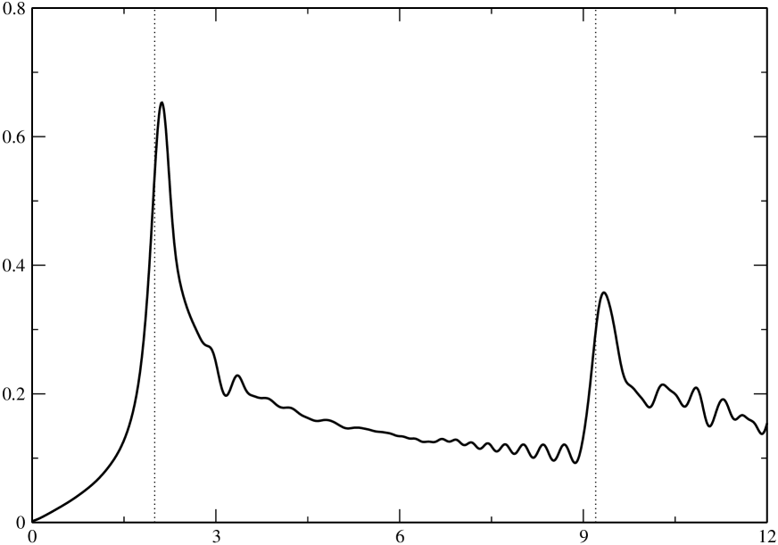
Figure 11: A convolution of the absolute value of the real part of the autocorrelation function (23) at $L=0$ with a normalized Gaussian in $\kappa$ of width 0.1, plotted as a function of $\kappa$ for the cosine perturbation with $N=597$, $\epsilon=1.5$ and $\theta=\pi/4$. Note the peaks associated with the tangent bifurcation (at $\kappa\approx 9.208$) and the second order bifurcation at ($\kappa=2$).

In Figure 9 (a) the real part of the autocorrelation function for $\kappa=\kappa^{\ast}=2$ is plotted and in (b) the deviation of the semiclassical approximation (35) from the exact expression (23) is shown. In Figure 10 the absolute value of the convolution of the autocorrelation function (22) with a normalized Gaussian is plotted as a function of $\kappa$ and $l$, showing the consistency of the theory: higher amplitudes near $l$-caustics and closed agreement with the predicted positions of the peak-centres (Figure 8). Finally, in Figure 11 the absolute value of the real part of the autocorrelation function (23) at $L=0$ (convolved with a Gaussian in $\kappa$ of width 0.1) is plotted. From this one sees clearly the influence of the two bifurcations: the tangent bifurcation at $\kappa\approx 9.208$ and the second order bifurcation at $\kappa=2$.

4 Acknowledgements

AB thanks the School of Mathematics, University of Bristol, and the Basic Research Institute in the Mathematical Sciences (BRIMS), Hewlett-Packard Laboratories, Bristol, for hospitality during the period when this work was started. SDP is grateful to Martin Sczyrba for helpful discussions, and to the School of Mathematics at the University of Bristol for hospitality and financial support. Support is also acknowledged from the Deutsche Forschungsgemeinschaft (for AB) and the Fundação de Amparo à Pesquisa do Estado do Rio Grande do Sul - FAPERGS (for SDP).

References

Arnold, V.I. 1978 Mathematical Methods in Classical Mechanics. Springer.

Bäcker, A. & Schubert, R. 2002 Amplitude distribution of eigenfunctions in mixed systems. J. Phys. A 35, 527-538 (BS1).

Bäcker, A. & Schubert, R. 2002 Autocorrelation function of eigenstates in chaotic and mixed systems. J. Phys. A 35, 539-564 (BS2).

Basílio de Matos, M. & Ozorio de Almeida, A.M. 1995 Quantization of Anosov maps. Ann. Phys. 237, 46-65.

Berry, M.V. 1977 Regular and irregular semiclassical wavefunctions J. Phys. A 10, 2083-2091.

Berry, M.V. 1989, Quantum scars of classical closed orbits in phase space. Proc. R. Soc. Lond. A 243, 219-231.

Berry, M.V, Keating, J.P & Prado, S.D. 1998 Orbit bifurcations and spectral statistics. J. Phys. A 31, L245-254.

Berry, M.V., Keating, J.P. & Schomerus, H. 2000 Universal twinkling exponents for spectral fluctuations associated with mixed chaology. Proc. R. Soc. Lond. A 456, 1659-1668.

Boasman, P.A. & Keating, J.P. 1995 Semiclassical asymptotics of perturbed cat maps. Proc. R. Soc. Lond. A 449, 629-653.

Bogomolny, E.B. 1988 Smoothed wavefunctions of chaotic quantum systems. Physica D 31, 169-189.

Gutzwiller, M.C. 1990 Chaos in Classical and Quantum Mechanics (New York: Springer).

Hannay, J.H. & Berry, M.V. 1980 Quantization of linear maps on the torus – Fresnel diffraction by a periodic grating. Physica D 1, 267-290.

Heller, E.J. 1984 Bound state eigenfunctions of classically chaotic Hamiltonian systems - scars of periodic orbits. Phys. Rev. Lett. 53, 1515-1518.

Kaplan, L. 1999 Scars in quantum chaotic wavefunctions. Nonlinearity 12, R1-R40.

Keating, J.P. 1991 The cat maps: quantum mechanics and classical motion. Nonlinearity 4, 309-341.

Keating, J.P., Mezzadri, F. & Robbins, J.M. 1999 Quantum boundary conditions for torus maps. Nonlinearity 12, 579-591.

Keating, J.P. & Prado, S.D. 2001 Orbit bifurcations and the scarring of wave functions. Proc. R. Soc. Lond. A 457, 1855-1872.

Li, B. & Rouben, D.C. 2001 Correlations of chaotic eigenfunctions: a semiclassical analysis. J. Phys. A 34, 7381-7391.

Mende, M. 1999 Periodic orbit bifurcations and spectral statistics. M.Sc. Thesis, University of Bristol.

Ozorio de Almeida, A.M. 1988 Hamiltonian Systems: Chaos and Quantization. Cambridge University Press.

Ozorio de Almeida, A.M. & Hannay, J.H. 1987 Resonant periodic orbits and the semiclassical energy spectrum. J. Phys A 20, 5873-5883.

Percival, I.C. 1973 Regular and irregular spectra. J. Phys. B 6, L229-L232.

Varga, I., Pollner, P. & Eckhardt, B. 1999 Quantum localization near bifurcations in classically chaotic systems. Ann. Phys. (Leipzig) 8, SI265-SI268.