Surface Quasigeostrophic Turbulence : The Study of an Active Scalar

Abstract

We study the statistical and geometrical properties of the potential temperature (PT) field in the Surface Quasigeostrophic (SQG) system of equations. In addition to extracting information in a global sense via tools such as the power spectrum, the g-beta spectrum and the structure functions we explore the local nature of the PT field by means of the wavelet transform method. The primary indication is that an initially smooth PT field becomes rough (within specified scales), though in a qualitatively sparse fashion. Similarly, initially 1D iso-PT contours (i.e., PT level sets) are seen to acquire a fractal nature. Moreover, the dimensions of the iso-PT contours satisfy existing analytical bounds. The expectation that the roughness will manifest itself in the singular nature of the gradient fields is confirmed via the multifractal nature of the dissipation field. Following earlier work on the subject, the singular and oscillatory nature of the gradient field is investigated by examining the scaling of a probability measure and a sign singular measure respectively. A physically motivated derivation of the relations between the variety of scaling exponents is presented, the aim being to bring out some of the underlying assumptions which seem to have gone unnoticed in previous presentations. Apart from concentrating on specific properties of the SQG system, a broader theme of the paper is a comparison of the diagnostic inertial range properties of the SQG system with both the 2D and 3D Euler equations.

I Introduction

In the Quasigeostrophic (QG) framework [1], a simplification of the Navier Stokes equations for describing the motion of a stratified and rapidly rotating fluid in a 3D domain, there are two classes of problems that immediately come to attention. The first (Charney type) are the ones where attention is focussed on the interior of the domain; the temperature is uniform along the boundaries and they play no dynamical role in the evolution of the system. The other class (Eady type) of problems lead to the Surface Quasigeostrophic (SQG) equations. The potential vorticity in the 3D interior is forced to be zero and the dynamical problem is controlled by the evolution of the potential temperature at the 2D boundaries. Working with a single lower boundary (assuming all fields to be well behaved as $z\rightarrow\infty$), the equations making up the SQG system can be expressed as [2],[3],

$${\partial}_{t}\theta+u^{i}{\partial}_{i}\theta=D_{t}\theta=0~{},z=0$$

$$\theta={\partial}_{z}\psi={(-\triangle)}^{\frac{1}{2}}\psi$$

$$\textrm{where}~{}~{}\nabla^{2}\psi=0,z>0~{}\textrm{and}~{}~{}\vec{u}={\nabla}^{\perp}\psi$$ (1)

Here $\theta$ is the potential temperature (it is a dynamically active scalar due to the coupling of $\theta$ to $\psi$), $\psi$ is the geostrophic streamfunction, $\vec{u}$ the geostrophic velocity, ${\nabla}^{\perp}\equiv(-{\partial}_{y},{\partial}_{x})$, $\triangle$ is the horizontal Laplacian, $\nabla^{2}$ is the full 3D Laplacian, the operator ${(-\triangle)}^{\frac{1}{2}}$ is defined [4] in Fourier space via $\widehat{{(-\triangle)}^{\frac{1}{2}}\psi(k)}=|k|\hat{\psi}(k)$ and $i=x,y$. Recall that the 2D Euler equations (for an incompressible fluid) in vorticity form are,

$${\partial}_{t}\xi+u^{i}{\partial}_{i}\xi=D_{t}\xi=0$$

$$\xi=\triangle\psi~{}\textrm{with}~{}\vec{u}={\nabla}^{\perp}\psi$$ (2)

where $\xi$ is the vertical component vorticity. The similarity in the evolution equations for $\theta$ and $\xi$ has been explored in detail by Constantin, Majda and Tabak [4],[5]. It can be seen that the structure of conserved quantities in both equations is exactly the same. To be precise, just as $f(\xi)$,$\int\psi\xi$ are conserved by the 2D Euler equations similarly $f(\theta)$,$\int\psi\theta$ are conserved in the SQG system. The basic difference in the above two systems is the degree of locality of the active scalar. For the 2D Euler equations the free space Green’s function behaves as $\ln{(r)}$ implying a $\frac{1}{r}$ behaviour for the velocity field due to point vortex at the origin. In contrast, in the SQG equations the free space Green’s function has the form $\frac{1}{r}$ implying a much more rapidly decaying $\frac{1}{r^{2}}$ velocity field due to a point "PT vortex" at the origin [2]. Or, in Fourier space one has $\hat{\xi}=|k|^{2}\hat{\psi}$ and $\hat{\theta}=|k|\hat{\psi}$ for the 2D Euler and SQG equations respectively [5]. Hence the nature of interactions is much more local in the SQG case as compared to the 2D Euler equations.

Studying the properties of active scalars with different degrees of locality would be an interesting question in its own right [6] but the specific interest in the SQG equations comes from an analogy with the 3D Euler equations. This can be seen by a comparison with the 3D Euler equations, which in vorticity form read,

$$[\frac{D{\omega}}{Dt}]^{j}=\partial_{i}v^{j}{\omega}^{i}$$ (3)

where $\vec{v}$ is a divergence free velocity field, $\vec{\omega}(=\nabla\times\vec{v})$ is the vorticity and $i,j=x,y,z$. Introducing $\vec{V}=\vec{{\nabla}^{\perp}\theta}$, a "vorticity" like quantity for the SQG system which satisfies (differentiating Eq. (1) and using incompressibilty),

$$[\frac{DV}{Dt}]^{j}=\partial_{i}u^{j}V^{i}$$ (4)

Identifying $\vec{V}$ in Eq. (4) with $\vec{\omega}$ in Eq. (3) it can be seen [4] that the level sets of $\theta$ are geometrically analogous to the vortex lines for the 3D Euler equations. Similar to the question of a finite time singularity in the 3D Euler equations (which is thought to be physically linked to the stretching of vortex tubes), in the SQG system one can think of a scenario where the intense stretching (and bunching together) of level set lines during the evolution of a front leads to the development of shocks in finite time. The issue of treating the SQG system as a testing ground for finite time singularities has generated interest [4],[5],[7],[8],[9] in the mathematical community and the reader is referred to the aforementioned papers for details regarding this issue.

In view of the similarities between the SQG and 2D Euler equations and the level set stretching analogy with the 3D Euler system, it is natural to inquire into the statistical/geometrical properties of the SQG active scalar within an appropriately defined "inertial range". The broad aim is to compare these properties with the large body of work available for the 2D and 3D Euler equations. In the second section we examine the PT field via global (power spectrum, structure functions, ($\beta,g(\beta)$) spectrum) and local (wavelets) methods. One of the few rigorous estimates that exist in fluid turbulence is that for the level set dimensions. The extraction of these dimensions and their agreement with analytical bounds is demonstrated. The third section is devoted to the examination of the dissipation field, the generalized dimensions of a measure based upon the dissipation field are calculated and commented upon. In the fourth section we focus our attention on the gradient fields, a simple derivation of the relation between the variety of scaling exponents is presented and the underlying assumptions are clearly stated. The failure of the cancellation exponent is demonstrated and a simple example is presented so as to put some of the ideas in perspective.

II The Potential Temperature Field

II.1 The Power Spectrum and the Structure Functions

A pseudo-spectral technique was employed to solve Eq. (1) numerically on a $2048\times 2048$ grid. Linear terms are handled exactly using an integrating-factor method, and nonlinear terms are handled by a third-order Adams-Bashforth scheme (fully de-aliased by the 2/3 rule method). The calculations were carried out for freely decaying turbulence. The initial conditions consisted of a large-scale random field, specifically a random-phase superposition of sinusoids with total wavenumber approximately equal to 6, in units where the gravest mode has unit wavenumber. Potential temperature variance is dissipated at small scales by $\nu\nabla^{2}\theta$ diffusion. Based on the typical velocity $U$ and scale $L$ of the initial condition, one may define a Peclet number $UL/\nu$. The calculations analyzed here were carried out for a Peclet number of 2500. After a short time, the spectrum develops a distinct inertial range. As time progresses, energy and $\theta$ variance are dissipated at small scales, the amplitude decreases, and the effective Peclet number also decreases. After sufficient time, the flow becomes diffusion-dominated and the inertial range is lost. Analysis of other cases, not presented here, indicates that the results are not sensitive to the time slice or the Peclet number, so long as the Peclet number is sufficiently large and the time slice is taken at a time when there is an extensive inertial range.

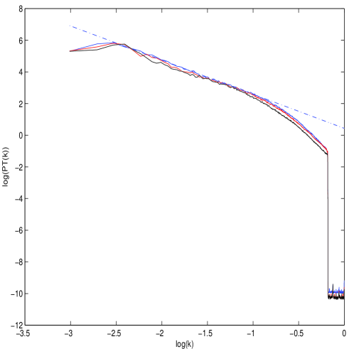
Figure 1: Power spectrum of the PT field for a variety of stages. The dashed line (extracted from the stage which has the largest inertial range) has a slope of $-2.15$.

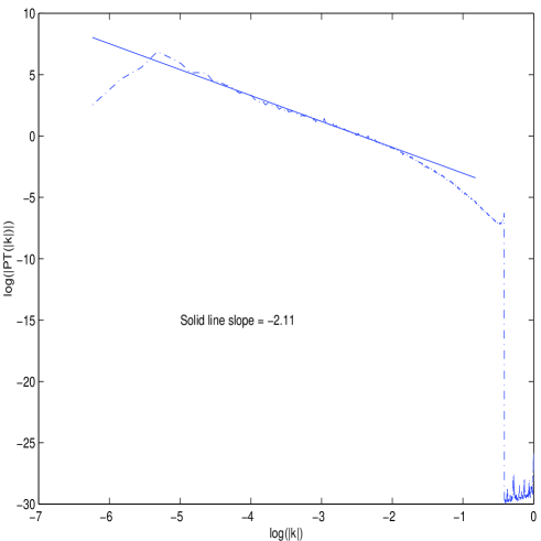
Figure 2: The 2D power spectrum for the stage with the largest inertial range. The solid line has a slope of $-2.11$.

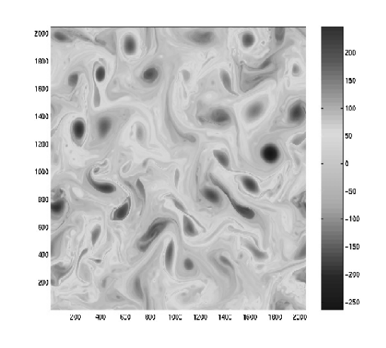
Figure 3: Snapshot of the PT field which showed the largest inertial range.

The mean 1D power spectra from different stages of evolution can be seen in Fig. 1. As these are decaying simulations the structure in the PT field is slowly dying out. The resulting increase in smoothness of the PT field can be seen via the roll off of the spectrum during the later stages. In spite of this a fairly clean power law is visible for a sizeable "inertial range" (other runs with large scale initial conditions posessing various amounts of energy show similar behavior). We choose to concentrate on the particular stage which has the largest inertial range. The 2D power spectrum for this stage can be seen in Fig. 2 and a snapshot of the PT field itself can be seen in Fig. 3. Interestingly the 2D power spectrum seems to roll off at larger wavenumbers as compared to the 1D spectrum. In this stage the spectral slope (from the 1D spectra) between the scales 256 to 8 (the scales are in terms of grid size) is $\approx-2.15$ (the other runs also showed slopes steeper than -2). The slope from the 2D spectrum is $\approx-2.11$ (due to the early roll off of the 2D spectrum, this slope is extracted between the scales 128 to 8). Previous decaying simulations [8] obtained values near $-2$ and seem to be consistent with our observations. A slope as steep as this suggests that the field being examined is smoother than expectations from a similarity hypothesis (which yields a $\frac{-5}{3}$ slope [3]). A closer look indicates (Fig. 3) that the field is composed of a small number of "coherent structures" superposed upon a background which has a filamentary structure consisting of very fine scales. This immediately brings to mind the studies on vorticity in decaying 2D turbulence [10],[11],[12] wherein a similar coherent structure/background picture was found to exist. Further analysis indicated that the vorticity field possessed normal scaling whereas a measure based upon the gradient of the vorticity (precisely the enstrophy dissipation) was multifractal. To proceed in this direction we introduce the generalized structure functions of order $q\in\Re^{+}$,

$$S_{q}(r)=<|\theta(x+r)-\theta(x)|^{q}>$$ (5)

Here $<.>$ represents an ensemble average. The directional dependence is suppressed due to the assumed isotropy of the PT field. Scaling behaviour in the field implies that one can expect the generalized structure functions to behave as [13],

$$S_{q}(r)=C_{1}(q){|\triangle\theta(L_{1})|}^{q}{(\frac{r}{L_{1}})}^{\zeta_{q}}~{};~{}r_{1}\leq r\leq L_{1}$$ (6)

where $\zeta_{q}$ are the generalized scaling exponents, $C_{1}(q)$ is of order unity for all $q$, $|\triangle\theta(L_{1})|$ is the absolute value of the difference in $\theta$ over a scale $L_{1}$. $r_{1}$ and $L_{1}$ are the inner and outer scale (8 and 256 respectively) over which the power law in the spectrum was observed.

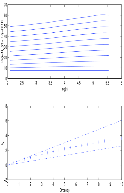
Figure 4: Upper Panel : $\log(S_{q}(r))$ Vs. $\log(r)$ for different values of q. Lower Panel : Scaling exponents for the PT field (+) and the linear scaling with $\beta_{min}$ and $\beta_{max}$.

If the field being examined is smooth at a scale $r$ then the gradient at this scale would be finite and as a consequence $\zeta_{q}=q$ (due to the domination of the linear term in the Taylor expansion about the point of interest) ie. the scaling would be trivial. Conventionally normal scaling is a term reserved for linear $\zeta_{q}$ and any nonlinearity in $\zeta_{q}$ is referred to as anomalous scaling. In 2D turbulence the velocity field is known to be smooth for all time if the initial conditions are smooth [14] and hence [15] $\zeta_{q}$(velocity)$=q$. Also, as mentioned, from the analysis of the vorticity field [10] the scaling exponents for the vorticity structure functions were found to depend on $q$ in a linear fashion. Plots of $\textrm{log}(S_{q}(r))$ Vs $\textrm{log}(r)$ for the PT can be seen in the upper panel of Fig. 4. In all cases the scaling is valid upto $r\sim 128$, using these plots we extracted $\zeta_{q}$ which are presented in the lower panel of Fig. 4. It is seen that the scaling is anomalous and in fact a best fit to the scaling exponents is of the form $\zeta_{q}=A{q}^{B},q>0$ with $B=0.82$.

For the special case of $q=2$, one can in principle relate the scaling exponent $\zeta_{2}$ to the slope of the power spectrum ($n$) via [16] $n=-(1+\zeta_{2})$. This relation is only valid for $-3<n<-1$ (note that this does not prevent the spectral slope from being steeper than $-3$; it just implies that $\zeta_{2}$ saturates at $2$ for smooth fields and the particular relation between $\zeta_{2}$ and $n$ breaks down). In our case $\zeta_{2}=1.05$ so the predicted spectral slope is $n=-2.05$ which is near the observed mean value of $-2.15$ (or $-2.11$ from the 2D spectrum). Even though the scaling exponents give an idea of the roughness in the field (anomalous scaling implying differing degrees of roughness) there is a certain unsatisfactory aspect about the structure functions, namely, there is no estimate of "how much" of the field is rough. The following subsection aims to address this very issue.

II.2 The $(\beta,g(\beta))$ spectrum

In scaling literature the roughness of a field is specified by means of an exponent $\beta$ ($>0$) defined as [17],

$$|\theta(x+r)-\theta(x)|\sim|r|^{\beta(x)}$$ (7)

Here $\beta$ is a function of position and it refers to the fact that the derivative of $\theta$ will be unbounded as $r\rightarrow 0$ if $\beta<1$. As mentioned previously there is a lower scale associated with the problem so technically nothing is blowing up and in effect $\beta<1$ represents the regions where the derivative will be large as compared to the rest of the field. Note that $\theta$ itself cannot be singular due its conserved nature. The focus is on whether an initially smooth $\theta$ field becomes rough so as to cause the gradient fields to experience a singularity. It is clear that Eq. (7) is by itself of not much use in characterizing $\theta$ (as $\beta$ depends upon position), in fact a global view of the specific degrees of rougness of $\theta$ can be attained via the $(\beta,g(\beta))$ spectrum which we introduce next.

An iso-$\beta$ set is defined as the set of all $x$’s where $\beta(x)=\beta$ and $g(\beta)$ is the dimension (to be precise $g(\beta)$ should be viewed in an probabilistic fashion [16]) of an iso-$\beta$ set. The dimensions of iso-$\beta$ sets are derived by Frisch [18]. Briefly, at a scale $r$ the probability of encountering a particular value of $\beta$ is proportional to $r^{d-g(\beta)}$ (where $d=2$ for the 2D PT field and $d=1$ for 1D cuts of the PT field). By using a steepest descent argument in the integral for the expectation value of $|\theta(x+r)-\theta(x)|^{q}$ one obtains [18],[16],

$$\zeta_{q}=\min_{\beta}[q\beta+d-g(\beta)]~{}\textrm{or}~{}g(\beta)=\max_{q}[q\beta+d-\zeta_{q}]$$ (8)

Hence given $\zeta_{q}$ for a fixed $q=q_{*}$ using the first part of Eq. (8),

$$q_{*}=\frac{dg(\beta)}{d\beta}$$ (9)

Denoting the value of $\beta$ for which Eq. (9) is satisfied by ${\beta}_{*}$ we have,

$$g({\beta}_{*})=d+q_{*}{\beta}_{*}-\zeta_{q_{*}}$$ (10)

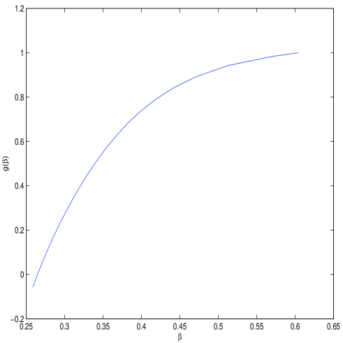
Figure 5: The $(\beta,g(\beta))$ spectrum

Notice that, as the structure functions involve moments with positive $q$, they only pick out ${\beta}$’s such that $\beta<1$ and $g(\beta)<d$. The $(\beta,g(\beta))$ spectrum seen in Fig. 5 hints at a hierarchy in roughness of the PT field. From the calculations we see that $\beta\in[0.26,0.6]$. In Fig. 4 along with $\zeta_{q}$ we have plotted the lines corresponding to $\zeta_{q}=q\beta_{min}$ and $\zeta_{q}=q\beta_{max}$. As is expected these lines straddle the actual scaling exponents. For smaller values of $q$ the scaling exponents are close to $q\beta_{max}$ as $\beta_{max}$ has the largest associated dimension whereas for higher values of $q$ the scaling exponents reflect the roughest regions and hence tend towards $q\beta_{min}$. Note that from Eq. (9) and Eq. (10) the approximation $\zeta_{q}=Aq^{B},B<1,q>0$ implies that $\beta$ becomes large and $g(\beta)\rightarrow d$ as $q\rightarrow 0$. In essence the picture that emerges is that even though $\theta$ appears to become rough (with differing degress of roughness), in fact, it is the smooth regions that occupy most of the space.

II.3 The roughness of $\theta$ : a qualitative local view

All of the previous tools, the power spectrum, the $(\beta,g(\beta))$ spectrum and the structure functions extracted information in a global sense. To get a picture of the actual positions where the signal may have unbounded derivatives, and to get a qualitative feel of the spareseness of these regions, one has to determine the local behaviour of the signal in question. Recently the use of wavelets has allowed the identification of local Holder exponents in a variety of signals. The Holder exponents are extracted by a technique known as the wavelet transform modulus maxima (WTMM) method [19],[20], [21],[22]. The modulus maxima refers to the spatial distribution of the local maxima (of the modulus) of the wavelet transform. In a crude sense the previous methods used ensemble averages of the moments of differences in $\theta(x)$ as "mathematical microscopes" whereas in the wavelet method it is the scale parameter of the wavelet transform that performs this task.

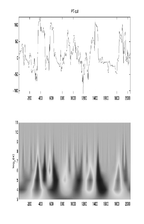
Figure 6: Upper Panel : A random 1D cut of the PT field. Lower Panel : Its wavelet transform (the analysing wavelet is the first derivative of a Gaussian), the cone like features indicate roughness in the analyzed signal.

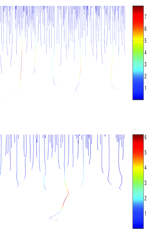
Figure 7: Upper Panel : The wavelet transform modulus maxima lines. The lower panel is a zoom into a particular section of the upper panel, this qualitatively indicates the sparseness of the rough spots. A log plot of the magnitude of the maxima line yields the local Holder exponent.

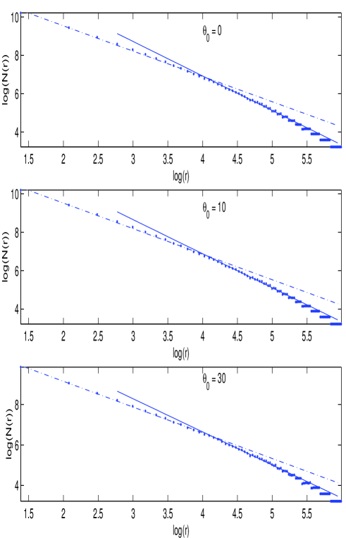
Figure 8: $\log(N(r))$ Vs. $\log(r)$ for 3 different level sets. The dashed line is the best fit for $4\leq r\leq 60$, the solid line is the best fit for $64\leq r\leq 200$. The box counting dimensions are $(1.32,1.8),(1.33,1.77)\textrm{and}(1.27,1.64)$ for the small and large $r$ regions for the 3 level sets respectively.

By using wavelets whose higher moments vanish one can detect sigularities in the higher order derivatives of the signal being analyzed [22]. Our previous results indicate that the PT field becomes rough, i.e., the first derivatives of the PT field should be unbounded. Hence, the particular wavelet we use is the first derivative of a Gaussian whose first moment vanishes [19],i.e., it picks up points where the signal becomes rough. The wavelet transform of a 1D cut of the PT field can be seen in Fig. 6. The cone like features imply the presence of a rough spot [22]. The modulus maxima lines are extracted from this transformed field and can be seen in Fig. 7. The value of the local Holder exponent can be extracted via a log plot of the magnitude of a particular maxima line [22]. In essence, the presence of the cones in the wavelet transform indicate roughness in the PT field and the WTMM lines locate the positions of the rough spots. However, a closer look (the lower panel of Fig. 7) suggests, qualitatively, that the rough regions are sparsely distributed (for eg. comparing with Fig. 8 in Arneodo et. al [20]). This goes along with the observation in the last subsection that the rough regions were non space filling. In contrast, it has been found [20],[21],[23] that the local Holder exponents ($h(x)$) associated with a 1D cut of the velocity field in 3D turbulence satisfy $-0.3\leq h(x)\leq 0.7$ for almost all $x$ (the peak of the histogram being at $\frac{1}{3}$) implying that the velocity field in 3D turbulence is very rough or has unbounded first derivatives at almost all points.

II.4 The Dimension of Level Sets

Apart from being physically interesting, the level set (iso-$\theta$ contour) dimensions provide another link to the roughness of the scalar field. As the initial condition was a smooth 2D field, initially, any given level set ($E_{\theta_{0}}$ for $\theta=\theta_{0}$) is a non space filling curve, i.e., the level set dimension ($D(E_{\theta_{0}})$) is one. In the case of 3D turbulence there exist analytical estimates of the scalar level set dimensions [24]. These estimates are seen to be numerically satisfied by a host of fields (both passive and active) in isotropic 3D and Magnetohydrodynamic (MHD) turbulence [25]. It must be emphasized that these estimates come directly from the equations of evolution and are much more powerful than the phenomenological ideas we have been working with so far. The actual calculation [24],[26] is of the area of an isosurface contained in a ball of specified size, given a Holder condition on the velocity field,

$$|u(x+y,t)-u(x,t)|\leq U_{L}{(\frac{y}{L})}^{\zeta_{u}}$$ (11)

this area estimate leads to the bound,

$$D(E_{\theta})\leq 2.5+\frac{\zeta_{u}}{2}$$ (12)

The bound in Eq. (12) is expected to be saturated [26] above a certain cutoff scale. A valid extrapolation [27] for the level sets of PT in the SQG system reads, $D(E_{\theta})\leq 1.5+(\zeta_{1})/2$, where $\zeta_{1}$ is given by Eq. (6) due to the equality of the scaling exponents for the velocity field and the PT in the SQG system.

In passing we mention that the analytical estimates are for the Hausdorff dimension whereas practically we compute the box counting dimension. We performed calculations for a variety of nominal (i.e., near the mean) level sets and Fig. 8 shows the log-log plots used in the calculation of the box counting dimension. As is the case for 3D [25],[24] there appears to be a crossover in $D(E_{\theta})$, we find that the even though the dimension undergoes a change, the fractal nature seems to persist at smaller scales. For small $r$, $D(E_{\theta})\approx 1.3$ whereas for larger values of $r$ we find $D(E_{\theta})\approx 1.74$ (see the caption of Fig. 8 for details on the actual values of $r$). >From our previous calculations $\zeta_{1}=0.57$, hence the analytical prediction is $D(E_{\theta})\leq 1.785$. Furthermore, as the bound is expected to be saturated above the cutoff we see that the computed value of $D(E_{\theta})$ for large $r$ is quite close to the analytical prediction. In all, apart from satisfying the analytically prescribed bounds (and indirectly indicating roughness in the PT field), the level set dimensions indicate that initially non space filling level sets acquire a fractal nature in finite time.

III Gradient Field Characterization

The effect of the inferred roughness in the PT field will, as mentioned previously, be reflected in the singular nature of the gradient fields. In this section we proceed to examine a variety of fields which are functions of the PT gradient. The aim is to see if we can actually detect the expected singularities, and if so, to characterize them.

III.1 The Dissipation Field

A physically interesting function of the gradient field is the PT dissipation, as it is connected to the variance of the PT field. The equation for the dissipation of $\theta$ can be obtained by multiplying Eq. (1) by $\theta$ and averaging over the whole domain,

$$\frac{\partial<\theta^{2}>}{\partial t}=-2\nu<(\nabla\theta)^{2}>$$ (13)

Here $\nu(\nabla\theta)^{2}$ is the dissipation field. Now consider the quantity $\mu(x,r)$,

$${\mu}(x,r)=\frac{1}{r^{d}}\int_{B(x,r)}{\nu(\nabla\theta)^{2}}d^{d}x$$ (14)

Physically this is the average dissipation in a ball of size $r$ centered at $x$. Due to the smoothing via integration it is expected that $\mu(x,r)$ will be fairly well behaved through most of the domain with intermittent bursts of high values concentrated in the regions where the PT field is rough. The multifractal formalism [28],[16] ,[29] provides a convenient way to characterize such "erratic" or singular measures. The technique [28] consists of constructing a measure ($\mu$ with suitable normalization) and using its moments to focus on the singularities of the measure. The domain in which the field is defined is partitioned into disjoint boxes of size $r$ and it is postulated (see for eg. [30]) that moments of $\mu$ will scale as,

$$\sum\mu(x,r)^{q}\sim r^{\tau_{q}-qd}$$ (15)

where the sum goes over all the boxes into which the domain was partitioned. Consider the set of points where the measure scales $r^{\alpha}$ and denote the dimension of this set by $f(\alpha)$ (again a probabilistic view is more precise). By similar considerations as for the $g(\beta)$ spectrum it can be seen that [16],

$$\tau_{q}=\min_{\alpha}(q\alpha-f(\alpha))~{}\textrm{and}~{}f(\alpha)=\max_{q}(q\alpha-\tau_{q})$$ (16)

The function $\tau_{q}$ is further related to the generalized dimensions [31] via $D_{q}=\tau_{q}/(q-1)$. Practically [29] a log-log plot of the ensemble average of $\mu(x,r)^{q}$ for different values of $r$ gives $(D_{q}-d)(q-1)$. By knowing $(q,D_{q})$ one can use Eq. (16) to obtain the $(\alpha,f(\alpha))$ spectrum.

Again, as we expect the scaling of any physical quantity to be restricted to a range of length scales (say $r_{a}$ to $r_{b}$), it is preferable to work in terms of ratios of $\frac{r}{r_{b}}$ where $r_{b}$ is the outer scale, $r_{a}$ is the inner scale and $r_{b}\geq r\geq r_{a}$. In these terms the generalized dimensions can be expressed as [29],

$$<{\mu(r)}^{q}>=C_{2}(q)({\mu(r_{b})}^{q}){(\frac{r}{r_{b}})}^{(D_{q}-d)(q-1)}$$ (17)

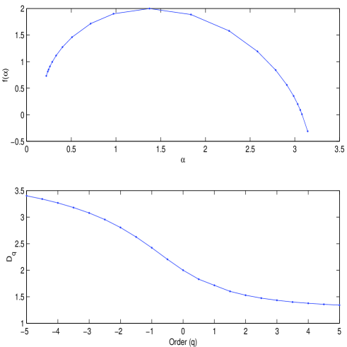
Figure 9: The $f(\alpha)$ spectrum and $D_{q}$ for the dissipation field

where $\mu(r_{b})$ is the measure on the outer scale and $C_{2}(q)$ is order unity for all $q$ (a similar relation would hold if we replaced the $({\mu(r_{b})}^{q})$ in the right hand side by $<{\mu(r)}>^{q}$ but with different $C_{2}(q)$’s). For $r<r_{a}$ the dissipation field is assumed to have become smooth via the action of viscosity. The $f(\alpha)$ spectrum and the generalized dimensions for the dissipation field can be seen in Fig. 9. The nontrivial behaviour of the generalized dimensions demonstrates that the dissipation field is singular (with different singularity strengths) within these scales. Also, from the calculations we find that $f(1)<2$ which acts as a check that the dissipation in a finite volume is bounded (as $f(1)$ is the dimension of the support of the singular regions) [32].

III.2 General Considerations

The gradient squared nature of the dissipation field implied that it was positive definite. In principle one could conceive of fields which possess singularities but aren’t sign definite. In order to characterize this possible sign indefiniteness Ott and co-workers studied [33],[34] sign singular measures and a related family of exponents called the cancellation exponents ($\kappa_{q}$). It is immediately clear that singular nature is a prerequisite for the phenomenon of cancellation, the reason being that a nonsingular field is bounded and we can always add a constant so as to make the field positive definite and hence eliminate cancellation. Consider a sign indefinite 1D field $\theta(x)$ (which will later be interpreted as a 1D cut of the PT field) and construct,

$${\mu}^{\prime}(x,r)=(\frac{1}{r}\int_{x}^{x+r}{|\frac{d\theta}{dx^{\prime}}|dx^{\prime}})~{};~{}$$ (18)

$${\eta}(x,r)=|\frac{1}{r}\int_{x}^{x+r}{(\frac{d\theta}{dx^{\prime}})dx^{\prime}}|$$ (19)

As ${\mu}^{\prime}$ is defined for the magnitude of the gradient field we can postulate (similar to Eq. (17) for $\mu$),

$$<{{\mu}^{\prime}(r)}^{q}>=C_{3}(q)({{\mu}^{\prime}(r_{d})}^{q}){(\frac{r}{r_{d}})}^{(D^{\prime}_{q}-d)(q-1)}$$ (20)

Here $d=1$ and $D^{\prime}_{q}$ are the generalized dimensions associated with ${\mu}^{\prime}$. As usual the scaling is restricted to a range of scales ($r_{c}<r<r_{d}$) and $r_{c}$ is the scale below which ${\mu}^{\prime}$ appears smooth. Formally, the entity $\eta$ after suitable normalization is a sign singular measure (see Ott et. al. [33] for a rigorous definition). It was conjectured [33] that the sign singular entity $\eta$ might also possess scaling properties in analogy with ${\mu}^{\prime}$, implying,

$$<{\eta}(r)^{q}>=C_{4}(q)(r)^{-{\kappa}^{\prime}_{q}}~{};~{}r>r_{cc}$$ (21)

Using Eq. (20) we can express Eq. (21) as,

$$<{\eta}(r)^{q}>\sim<{{\mu}^{\prime}}(r)^{q}>(r)^{-\kappa_{q}}~{};~{}r_{d}>r>r_{cc}\geq r_{c}$$ (22)

Where $\kappa_{q}={\kappa}^{\prime}_{q}+(D^{\prime}_{q}-d)(q-1)$ and $r_{cc}$ is the lower oscillatory scale below which the derivative does not oscillate. We prefer to call $\kappa_{q}$ from Eq. (22) the cancellation exponents as they directly reflect the difference in the scaling properties of $\frac{d\theta}{dx}$ and $|\frac{d\theta}{dx}|$.

Apriori there is no justification in assuming that the scale at which cancellation ceases ($r_{cc}$) is the same as the scale at which ${\mu}^{\prime}$ becomes smooth ($r_{c}$). Consider the example where the derivative is a discrete signal composed of a train of delta functions (zero elsewhere) where the minimum separation between the delta functions is $l$. Furthermore let us assign the sign of the delta functions in a random fashion. In this case the $r_{cc}=l$, in fact, $\kappa_{1}=0.5$ due to the random distribution of the signs. But as the delta functions are supported at points we have $r_{c}\rightarrow 0$. As an aside we point out that if there is a maximum scale of separation between the delta functions (say $L$) then at scales greater than $L$ we will see $D^{\prime}_{q}=d$ for ${\mu}^{\prime}$. The reason for pointing this out is to give a feel for fields that exhibit scaling, on one hand smooth fields have $D^{\prime}_{q}=d$ whereas on the other extreme random fields with small correlations also have $D^{\prime}_{q}=d$ (at scales larger than their correlation lengths). Fields with nontrivial scaling over a significant range are in effect random but with large correlation lengths. The reader is referred to Marshak et. al. [35] for a detailed examination of multiplicative processes and the resulting characterization by structure functions and generalized dimensions.

In order to get a unified picture of scaling in both the gradient and the field itself there have been attempts (for eg. [13],[17]) to link $\zeta_{q}$, $\kappa_{q}$ and $D^{\prime}_{q}$ to each other. The view that seems to have emerged is that there exist simple relations linking the various exponents and that these relations are valid under very general conditions. We present an alternate derivation of some of these relations which makes the implicit assumptions explicit. Proceeding from Eq. (22), assuming that $\frac{d\theta}{dx}$ has integrable singularities we obtain,

$$<|\theta(x+r)-\theta(x)|^{q}>=<{{\mu}^{\prime}}(r)^{q}>r^{q-\kappa_{q}}$$ (23)

Substituting from Eq. (20) and on comparing with Eq. (6) we get,

$$\zeta_{q}=(D^{\prime}_{q}-d)(q-1)+q-\kappa_{q}$$ (24)

Writing Eq. (23) for $q=1$ we have,

$$<|\theta(x+r)-\theta(x)|>=<{{\mu}^{\prime}}(r)>r^{1-\kappa_{1}}$$ (25)

which yields $\kappa_{1}+\zeta_{1}=1$. Now if we make a strong assumption regarding the uniform nature of the cancellation, it is possible to claim that Eq. (25) holds not only in average but on every interval, ie,

$$|\theta(x+r)-\theta(x)|={{\mu}^{\prime}}(r)r^{1-\kappa_{1}}$$ (26)

Raising this to the $q^{th}$ power and performing an ensemble average yields,

$$<|\theta(x+r)-\theta(x)|^{q}>=<{{\mu}^{\prime}}(r)^{q}>r^{q(1-\kappa_{1})}$$ (27)

which implies,

$$\zeta_{q}=(D^{\prime}_{q}-d)(q-1)+q(1-\kappa_{1})$$ (28)

The implications of Eq. (28) are quite severe in that it shows $\zeta_{q}$ to be dependent on $D^{\prime}_{q}$ and the knowledge of only the first cancellation exponent allows the derivation of one from the other. In general the scaling exponents of $\theta$ and the generalized dimensions of ${\mu}^{\prime}$ provide exclusive information. It is only in the presence of integrable singularities that one can link the two via Eq. (24), furthermore the stronger relation (Eq. (28)) is valid under the added assumption of uniform cancellation.

III.3 The Gradient of the PT and its absolute value

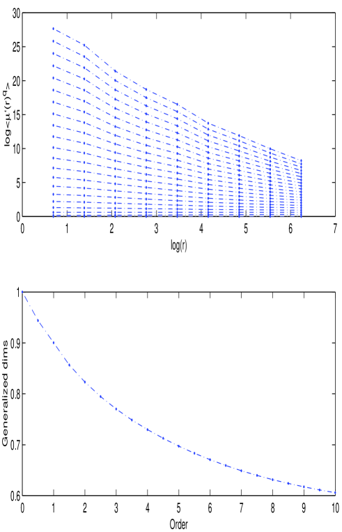
Figure 10: Upper Panel : $\textrm{log}(<{\mu}^{\prime}(r)^{q}>)$ Vs. $\textrm{log}(r)$ for $q=1:10$, Lower Panel : The generalized dimensions for ${\mu}^{\prime}$

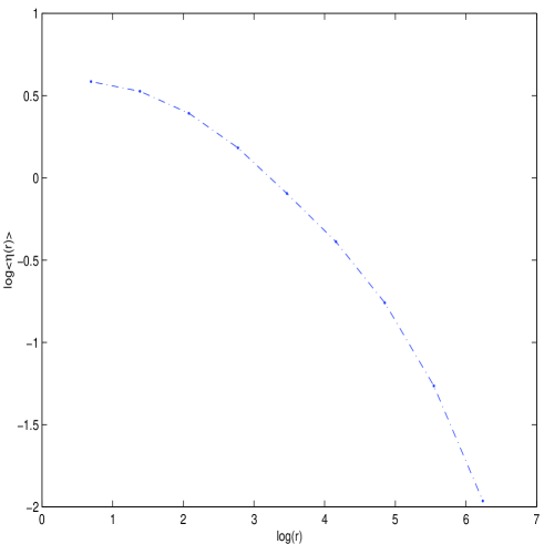
Figure 11: $\textrm{log}(<{\eta}(r)>)$ Vs. $\textrm{log}(r)$

We proceed to check if scaling is observed (as postulated) for the PT field gradient and its absolute value and whether one can extract the aforementioned exponents. In the upper panel of Fig. 10 we show the log-log plots of $<{\mu}^{\prime}(r)^{q}>$ Vs. $r$ for different $q$. The scaling relations certainly appear to hold true (which was expected as they held for the dissipation field). The generalized dimensions for ${\mu}^{\prime}$ can be seen the lower panel of Fig. 10. On the other hand the scaling for $<{\eta}(r)>$ seen in Fig. 11 fails to exhibit a power law in $r$. Hence there is no meaningful way of extracting the cancellation exponents as they have been defined. Unfortunately this implies that the relations derived in the previous section (Eqs. (24) and (28)) cannot be used in this situation. In spite of this, we can see that as $r$ decreases the tangent to $\textrm{log}(<{\eta}(r)>)$ has a smaller slope which is consitent with the existence of a oscillatory cutoff at small scales.

IV Conclusion and Discussion

In summary, we have found that the PT field in the SQG equations appears to become rough within a specified range of scales. Moreover, not only is there a heirarchy in the degree of roughness, the roughness is distributed sparsely in a qualitative sense. These conclusions are based on a combination of factors, namely, the algebraic power spectrum, anomalous scaling in the structure functions, a nontrivial $(\beta,g(\beta))$ spectrum, the nature of the WTMM map and the wrinkling of the PT level sets. The roughness in the PT field is expected to have an adverse effect on functions of the gradient field. This expectation is bourne out in the multifractal nature of the dissipation field. Also, the singular nature of the gradient field in combination with its sign indefinetness led us to examine a sign singular measure based upon the gradient field. The failure to observe scaling in the sign singular measure serves, in our opinion, as a reminder that most scaling arguments are postulated at a phenomenological level and the underlying basis of why scaling is observed in the first place is a fairly subtle and unsettled issue. Similarly the simple derivation of the relation between the variety of scaling exponents makes explicit some of the assumptions that are required for the validity of similar relations proposed in earlier studies.

Regarding the more general question we posed in the very beginning of this paper, i.e., where does the SQG active scalar stand with respect to both 2D and 3D turbulence, we have the following comments. With respect to the vorticity in the 2D Euler equations the corresponding quantity in the SQG system is the PT. The coherent structure/fine background nature of the vorticity field [10],[11],[12] carries over qualitatively to the PT field. The vorticity structure functions which showed normal scaling in the 2D Euler system [10] cross over to anomalous scaling in the SQG system. Our conjecture is that the stronger local interactions in the SQG system are responsible for this anomalous scaling. In both these systems the vorticity and PT respectively are conserved quantities and hence any singularities one might experience are actually in the gradient fields, as is seen in the multifractal nature of the enstrophy dissipation in the Euler system [10] and the PT dissipation in the SQG system.

In the 3D Euler case, the PT from the SQG equations is analogous to the velocity field and $\vec{{\nabla}^{\perp}\theta}$ from SQG corresponds to the vorticity of the 3D Euler equations. The roughness of the PT field is similar to the postulated roughness of the velocity field in the inertial range, a subtle difference being that the roughness in the PT appears to be sparse whereas indications are that the roughness in the 3D velocity field is present almost everywhere [20],[21],[23]. We re-emphasize that in both these cases the roughness is restricted to a range of scales, i.e., no claim is made for an actual singularity in the corresponding gradients. Similarly the anomalous scaling of the PT follows that of the velocity field in 3D but again it is not as strong as in the 3D case. The general theory developed [24] for the deformation of scalar level sets in the 3D case is seen to carry over to the SQG equations. In essence the SQG equations follow the 3D Euler equations but in a somewhat weaker sense. This "weakness" is clearly manifested in the behaviour of the gradients. In the 3D Euler equations a sign singular measure constructed from the vorticity field shows good scaling properties and a cancellation exponent can be meaningfully extracted [33], whereas in the SQG equations a similarly constructed entity lacks scaling.

The results presented in this paper have been for the most part diagnostic, in that they characterize the nature of the roughness of the potential temperature field in SQG dynamics. Although we have exhibited anomalous scaling of the potential temperature fluctuations, we do not have a theory accounting for the observed form of $\zeta_{q}$. Arriving at such a theory will be a major challenge for future work. Our results point efforts in the direction of considering the dichotomy between smooth fields within large organized vortices, and a rather sparse set at the boundaries of and between vortices which exhibits a greater degree of roughness. The diagnostic results also suggest a means for distinguishing between SQG and Euler dynamics in Nature, in cases where only a tracer field can be observed, as in the gas giant planets (notably Saturn, Jupiter and Neptune, which exibit a rich variety of turbulent patterns). SQG dynamics should yield anomalous scaling corresponding to sparse roughness, whereas Euler dynamics should yield normal scaling.

- [1] J. Pedlosky. Geophysical Fluid Dynamics, Springer Verlag, Chapter 6, 1979.
- [2] I. Held, R. Pierrehumbert, S. Garner and K. Swanson. Surface quasi-geostrophic dynamics, Journal of Fluid Mechanics, 282, 1, 1995.
- [3] R. Pierrehumbert, I. Held and K. Swanson. Spectra of Local and Nonlocal Two-dimensional Turbulence, Chaos, Solitons and Fractals, 4, 6, 1111, 1995.
- [4] P. Constantin, A. Majda and E. Tabak. Formation of strong fronts in the 2D quasigeostrophic thermal active scalar, Nonlinearity, 7, 1495, 1994.
- [5] A. Majda and E. Tabak. A two-dimensional model for for quasigeostrophic flow: comparison with two-dimensional Euler flow, Physica D, 98, 515, 1996.
- [6] N. Schorghofer. Energy spectra of steady two-dimensional turbulent flows, Physical Review E, 61, 6572, 2000.
- [7] P. Constantin, Q. Nie and N. Schorghofer. Front formation in an active scalar equation, Physical Review E, 60, 3, 2858, 1999.
- [8] K. Okhitani and M. Yamada. Inviscid and inviscid-limit behaviour of a surface quasigeostrophic flow, Physics of Fluids, 9, 4, 876, 1997.
- [9] D. Cordoba and C. Fefferman. Behaviour of several two-dimensional fluid equations in singular scenarios, Proc. Nat. Acad. Sci. USA, 98, 4311, 2001.
- [10] R. Benzi and R. Scardovelli. Intermittency of Two-Dimensional Decaying Turbulence, Europhys. Lett., 29, 5, 371, 1995.
- [11] R. Benzi, G. Paladin, S. Patarnello, P. Santangello and A. Vulpiani. Intermittency and coherent structures in two-dimensional turbulence, J. Phys. A : Math. Gen., 19, 3371, 1986.
- [12] H. Mizutani and T. Nakano. Multifractal Analysis of Simulated Two-Dimensional Turbulence, Journal of the Physical Society of Japan, 58, 5, 1595, 1989.
- [13] S. Vainshtein, K. Sreenivasan, R. Pierrehumbert, V. Kashyap and A. Juneja. Scaling exponents for turbulence and other random processes and their relationships with multifractal structure, Physical Review E, 50, 3, 1823, 1994.
- [14] H. Rose and P. Sulem. Fully Developed Turbulence and Statistical Mechanics, J. Phys. Paris, 47, 441, 1978.
- [15] R. Benzi, G. Paladin and A. Vulpiani. Power spectra in two-dimensional turbulence, Physical Review A, 42, 6, 3654, 1990.
- [16] U. Frisch. Turbulence, Cambridge Press, 1995.
- [17] A. Bertozzi and A. Chhabra. Cancellation exponents and fractal scaling, Physical Review E, 49, 5, 4716, 1994.
- [18] U. Frisch. From global scaling, a la Kolmogorov, to local multifractal scaling in fully developed turbulence, Proc. R. Soc. Lond. A, 434, 89, 1991.
- [19] J. Muzy, E. Bacry and A. Arneodo. Multifractal formalism for fractal signals: The structure-function approach versus the wavelet-transform modulus-maxima method, Physics Review E, 47, 2, 875, 1993.
- [20] A. Arneodo, E. Bacry and J. Muzy. The thermodynamics of fractals revisited with wavelets, Physica A, 213, 232, 1995.
- [21] J. Muzy, E. Bacry and A. Arneodo. Wavelets and Multifractal Formalism for Singular Signals: Application to Turbulence Data, Physical Review Letters, 67, 25, 3515, 1991.
- [22] S. Mallat and W. Hwang. Singularity Detection and Processing with Wavelets, IEEE Trans. on Information Theory, 38, 2, 617, 1992.
- [23] K. Daoudi. A New Approach for Multifractal Analysis of Turlbulence Signals, Fractals and Beyond, M. Novak Ed., World Scientific, 91, 1998.
- [24] P. Constantin, I. Proccacia and K. Sreenivasan. Fractal Geometry of Isoscalar Surfaces in Turbulence: theory and experiments, Physical Review Letters, 67, 13, 1739, 1991.
- [25] A. Brandenburg, I. Proccacia, D. Segel and A. Vincent. Fractal level sets and multifractal fields in direct simulation of turbulence, Physical Review A, 46, 8, 4819, 1992.
- [26] P. Constantin and I. Proccacia. Scaling in fluid turbulence : A geometric theory, Physical Review E, 47, 5, 3307, 1993.
- [27] P. Constantin. Personal communication.
- [28] T. Halsey, M. Jensen, L. Kadanoff, I. Procacia and B. Shraiman. Fractal measures and their singularities: the characterization of strange sets, Physics Review A, 33, 1141, 1986.
- [29] C. Meneveau and K. Sreenivasan. The multifractal nature of turbulent energy dissipation, Journal of Fluid Mechanics, 224, 429, 1991.
- [30] I. Hosokawa. Theory of scale-similar intermittant measures, Proc. Roy. Soc. London A, 453, 691, 1997.
- [31] H. Hentschel and I. Procaccia. The infinite number of generalized dimensions of fractals and strange attractors, Physica D, 8, 435, 1983.
- [32] K. Sreenivasan and C. Meneveau. Singularities of the equations of fluid motion, Physical Review A, 38, 12, 6287, 1988.
- [33] E. Ott, Y. Du, K. Sreenivasan, A. Juneja and A. Suri. Sign-Singular Measures: Fast Magnetic Dynamos, and High-Reynolds-Number Fluid Turbulence, Physical Review Letters, 69, 18, 2654, 1992.
- [34] Y. Du, T. Tel and E. Ott. Characterization of sign-singular measures, Physica D, 76, 168, 1994.
- [35] A. Marshak, A. Davis, R. Cahalan and W. Wiscombe. Bounded cascade models as nonstationary multifractals, Physics Review E, 49, 1, 55, 1994.