Stochastic ionization through noble tori : Renormalization results

Abstract

We find that chaos in the stochastic ionization problem develops through the break-up of a sequence of noble tori. In addition to being very accurate, our method of choice, the renormalization map, is ideally suited for analyzing properties at criticality. Our computations of chaos thresholds agree closely with the widely used empirical Chirikov criterion.

The multiphoton ionization of hydrogen in a strong microwave field [1] revolutionized traditional notions about the physics of highly excited atoms. Its interpretation remained a puzzle until its stochastic, diffusional nature was uncovered through the then-new theory of chaos [2] thereby making it the most important testing ground for quantal manifestations of classical chaos [3]. The onset of chaos in that problem has been the focus of intensive research and is generally believed to be induced by the break-up of invariant tori  [4], which act as barriers in phase space preventing the diffusion of trajectories for Hamiltonian systems with two degrees of freedom.

Over the last two decades, different methods to estimate break-up thresholds of invariant tori have been developed and applied to various physical models with two effective degrees of freedom: Chirikov’s resonance overlap criterion [5], its empirical “2/3-rule” version [6], and Escande-Doveil renormalization [7]. These methods provide merely approximate values (as compared to direct numerical integration) even though Escande-Doveil renormalization is known to give very accurate values in some concrete examples. Systematic methods are now available to obtain very accurate values, such as, e.g., Greene’s residue criterion [8], Laskar’s frequency map analysis [9, 10], or renormalization analysis [11, 12, 13, 14]. There is numerical evidence that these independent and systematic methods give the same values for the chaos thresholds [12, 14, 15]. However, renormalization has an additional advantage : By focusing on specific tori, it leads to very accurate thresholds, and allows one to analyze the properties at criticality. Indeed, the renormalization map can be likened to a phase space microscope by which the system can be studied with larger and larger magnification.

In this article, we find the transition to chaos in the hydrogen atom driven by circularly polarized microwaves using renormalization. This problem has emerged as paradigm for a number of issues in multi-dimensional nonlinear dynamics (see Ref. [16] and references therein). Our results reveal that the onset of chaos in the microwave problem develops through a sequence of “noble” tori, i.e. tori with frequency equivalent to the golden mean $\gamma=(\sqrt{5}-1)/2$.

Furthermore, the chaos thresholds obtained by the renormalization are in very good agreement with the 2/3-rule criterion [17, 18, 19], and better than the ones obtained by the Escande-Doveil renormalization [19]. In this model, Chirikov’s criterion can be used to determine very accurate critical thresholds of ionization (accurate to 5%) for most values of the parameter (eccentricity of the initial orbit).

Renormalization method–

The renormalization method is based on the construction of successive canonical transformations [11, 13, 14]. In its most recent version, it acts on the following family of Hamiltonians with two degrees of freedom written in actions $\boldsymbol{A}=(A_{1},A_{2})$ and angles $\boldsymbol{\varphi}=(\varphi_{1},\varphi_{2})$ :

$$H(\boldsymbol{A},\boldsymbol{\varphi}) = \boldsymbol{\omega}\cdot\boldsymbol{A}+V(\boldsymbol{\Omega}\cdot\boldsymbol{A},\boldsymbol{\varphi})$$ (1)

$$= \boldsymbol{\omega}\cdot\boldsymbol{A}+\sum_{\boldsymbol{\nu}\in{\mathbb{Z}}^{2}\atop k\in{\mathbb{N}}}V_{k,\boldsymbol{\nu}}(\boldsymbol{\Omega}\cdot\boldsymbol{A})^{k}e^{i\boldsymbol{\nu}\cdot\boldsymbol{\varphi}},$$ (2)

where $\boldsymbol{\omega}=(\omega,-1)$ is the frequency of the invariant torus, and $\boldsymbol{\Omega}=(1,\alpha)$ is some other vector. Two steps are involved [20] : an elimination of the non-resonant modes $\boldsymbol{\nu}$ of the Hamiltonian (the modes which do not involve small denominator problems), and a rescaling of phase space (shift of the resonances, rescaling in time and in the actions). This transformation reduces to a map ${\mathcal{R}}$ of Fourier coefficients $(\omega^{\prime},\alpha^{\prime};\{V^{\prime}_{k,\boldsymbol{\nu}}\})={\mathcal{R}}(\omega,\alpha;\{V_{k,\boldsymbol{\nu}}\})$.

The main conjecture of the renormalization approach is that if the torus exists for a given Hamiltonian $H$, the iterates ${\mathcal{R}}^{n}H$ of the renormalization map acting on $H$ converge to some integrable Hamiltonian $H_{0}$. This conjecture is supported by analytical results in the perturbative regime [20, 21], and by numerical results [15, 14]. For a one-parameter family of Hamiltonians $\{H_{F}\}$, the critical amplitude of the perturbation $F_{c}(\omega)$ is determined by the following conditions :

$${\mathcal{R}}^{n}H_{F}\underset{n\to\infty}{\to}H_{0}(\boldsymbol{A})=\boldsymbol{\omega}\cdot\boldsymbol{A}+\frac{1}{2}(\boldsymbol{\Omega}\cdot\boldsymbol{A})^{2}\quad\mbox{ for }F<F_{c}(\omega),$$ (3)

$${\mathcal{R}}^{n}H_{F}\underset{n\to\infty}{\to}\infty\quad\mbox{ for }F>F_{c}(\omega).$$ (4)

Model–

We consider a hydrogen atom interacting with a strong microwave field of amplitude $F$ and frequency $\Omega$, circularly polarized in the orbital plane. In action-angle variables, the classical Hamiltonian is reduced to the following Hamiltonian with two degrees of freedom [18] :

$$H(J,L,\theta,\psi)=-\frac{1}{2J^{2}}-\Omega L+F\sum_{n=-\infty}^{+\infty}V_{n}(J,L)\cos(n\theta+\psi),$$ (5)

where

$$V_{0}(J,L)=-\frac{3e}{2}J^{2},$$

$$V_{n}(J,L)=\frac{1}{n}\left[{\mathcal{J}}^{\prime}_{n}(ne)+\frac{\sqrt{1-e^{2}}}{e}{\mathcal{J}}_{n}(ne)\right]J^{2},\,\mbox{ for }n\not=0,$$

where ${\mathcal{J}}_{n}$ is the $n$th Bessel function of the first kind and ${\mathcal{J}}_{n}^{\prime}$ is its derivative. The angles $\theta$ and $\psi$ are conjugate to the principal action $J$ and to the angular momentum $L$ respectively. The eccentricity $e$ of the initial orbit is given by $e=(1-L^{2}/J^{2})^{1/2}$. Hamiltonian (5) can be rescaled in order to eliminate the dependence on the frequency of the microwave field. We rescale time by a factor $\Omega$ [we divide Hamiltonian (5) by $\Omega$]. We rescale the actions $J$ and $L$ by a factor $\lambda=\Omega^{1/3}$, i.e. we replace $H(J,L,\theta,\psi)$ by $\lambda H(J/\lambda,L/\lambda,\theta,\psi)$. We notice that this rescaling does not modify $e(J,L)$. The resulting Hamiltonian becomes :

$$H=-\frac{1}{2J^{2}}-L+F^{\prime}\sum_{n=-\infty}^{+\infty}V_{n}(J,L)\cos(n\theta+\psi),$$

where $F^{\prime}=F\Omega^{-4/3}$ is the rescaled amplitude of the field. In what follows we assume that $\Omega=1$.

For the unperturbed Hamiltonian (5), i.e. with $F=0$, we consider a motion with Kepler frequency $\omega\in[-1,1]$ (the high scaled frequency regime). In phase space, this trajectory evolves on a two-dimensional torus. If $\omega$ is irrational, the trajectory fills the torus densely. This invariant torus is located at $J=\omega^{-1/3}$ and $L=-E_{0}-\frac{1}{2}\omega^{2/3}$, where $E_{0}$ is the total energy of the system (in the rotating frame). For convenience, we shift the action $J$ such that the torus is located at $J=0$, and we expand the resulting Hamiltonian in Taylor series in the action $J$. Furthermore, we rescale the actions $J$ and $L$ by a factor $\lambda=-3\omega^{4/3}$, making Hamiltonian (5) :

$$H_{F}=\omega J-L+\sum_{k=2}^{+\infty}\frac{k+1}{6(3\omega)^{k-2}}J^{k}+F\left(-\frac{1}{3}\omega^{-4/3}J^{2}+2\omega^{-1/3}J-3\omega^{2/3}\right)\sum_{n=-\infty}^{+\infty}\tilde{V}_{n}(e)\cos(n\theta+\psi),$$ (6)

where $\tilde{V}_{n}(e)=V_{n}(1,\sqrt{1-e^{2}})$. We note that the rescaling coefficient $\lambda$ has been chosen such that the quadratic part of the Hamiltonian is $J^{2}/2$. The resulting Hamiltonian conforms to (1) with $\alpha=0$ and with coordinates $\boldsymbol{A}=(J,L)$ and $\boldsymbol{\varphi}=(\theta,\psi)$.

In what follows, we consider $e$ (the eccentricity of the initial orbit) as a parameter of the system. For $e=1$, the resulting model is a one-dimensional hydrogen atom in a linearly polarized microwave field [3]. By varying $e$, we obtain a wide variety of models where we can compare renormalization and empirical rules.

Breakup thresholds of invariant tori–

For a given eccentricity $e$, we compute the critical function $F_{c}(\omega;e)$ using the renormalization method [Eqs. (3)-(4)]. Figure 1 shows a typical critical function $\omega\mapsto F_{c}(\omega;e)$ for $e=0.45$ and for co-rotating orbits ($\omega>0$). The critical function vanishes at all rational values of the frequency (since all tori with rational frequency are broken as soon as the field is turned on), and it is discontinuous on a dense set. This figure shows that there is no invariant torus between the resonances 1:1 and 4:1 for $F_{c}>\max_{\omega\in[1/4,1]}F_{c}(\omega;e=0.45)\approx 0.0069$. The most stable region is located around $\omega\approx 0.723$.

Figure 2 shows the critical thresholds between two primary resonances $\max_{\omega\in[1/2,1]}F_{c}(\omega,e)$ and $\max_{\omega\in[1/3,1/2]}F_{c}(\omega,e)$ as a function of the parameter $e$ for co-rotating ($\omega>0$) and for counter-rotating ($\omega<0$) orbits. This figure is analogous to Fig. 3 of Ref. [19]. In a broad range of values of $e$ ($e\in[0.2,1]$) the heuristic 2/3-rule criterion gives very accurate results (accurate to 5%) by comparison with our renormalization results for co-rotating orbits. The values are even better than the ones computed by Escande-Doveil renormalization [19]. However, for very low eccentricity, there is a large gap between both results which makes the 2/3-rule inapplicable in this range of parameter $e$. For this case, Escande-Doveil renormalization is a better criterion for the determination of the thresholds. As $e$ tends to zero, the discrepancy is even bigger. For instance, for the overlap between $1:1$ and $2:1$, the 2/3-rule criterion predicts a finite value of the threshold at $e=0$ whereas Hamiltonian (6) is integrable in that case and the critical function is expected to go to infinity at $e=0$.

For counter-rotating orbits, the 2/3-rule criterion overestimates the critical couplings even though it gives fairly accurate results (less than 10% for $e\in[0.8,1]$). The resulting critical curve is below what has been obtained in Ref. [19] using the Escande-Doveil renormalization with a discrepancy around 30%.

Our results confirm that the orbits with medium eccentricity can diffuse more easily between the first primary resonances ($n=1,2,3$) [19]. However, in order to ionize, the orbits must diffuse throughout phase space or at least between a large number of primary resonances $n_{c}^{q}$ (in experiments and numerical simulations [22], $n_{c}^{q}\approx 40$). Since the 2/3-rule gives very accurate results in a broad range of parameter $e$, we compute the critical thresholds between resonances $m$:1 and $m$+1:1 for $m=1,\ldots,n_{c}^{q}$ with $n_{c}^{q}=40$, for medium and large eccentricities. In Fig. 3 we have plotted the different critical curves $e\mapsto\max_{\omega\in[1/(m+1),1/m]}F_{c}(\omega;e)$ for $m=1,\ldots,n_{c}^{q}$ for co-rotating and counter-rotating orbits. It appears that there is a very broad region of the parameter $e$ where an orbit cannot diffuse from the resonance 1:1 to $n_{c}^{q}$:1. In fact, only in the region $e\in[0.9,1]$ (with $F>0.015$ for co-rotating orbits, or with $F>0.05$ for counter-rotating ones), the orbits can ionize. In other terms, only the high-eccentricity orbits can ionize in this classical model (6). This observation reinforces the importance of core collisions for the ionization process [16].

A more commonly used function is the scaled function $F_{0}(\omega)=F_{c}(\omega)\omega^{-4/3}$. For the linearly polarized case ($e=1$), experiments [23] and numerical computations [24] show that for $F_{0}=F_{c}n^{4}>0.02$ (when $n$ is the principal quantum number) there is ionization for $\Omega_{0}=1/\omega$ (the scaled frequency) close to 1. Here we find agreement with this value: for $F_{0}>0.022$, there is no invariant curve in phase space and diffusion can occur. For the circularly polarized case ($e\not=1$), the conclusions are less clear. However since there is a broad stable region $e\in[0,0.8]$, we expect the circularly polarized driven atoms to ionize less easily than the linearly driven ones. Since the orbits of high eccentricities are the ones which ionize, we expect the behavior of ionization curves for circularly polarized microwaves to be similar to the ones for linearly polarized ones. This is consistent with experiments (Fig. 1 of Ref. [22]).

Progress to chaos through noble tori–

The renormalization map allows us to determine accurately the frequency of the last invariant torus to break-up. The conventional wisdom is that the last invariant torus surviving with increasing the amplitude of the perturbation is the one with frequency equal to the golden mean $\gamma=(\sqrt{5}-1)/2$. The example we study shows that this belief is mistaken. Figure 4 shows the value of the frequency of the last invariant torus between resonances 1:1 and 2:1, and between 2:1 and 3:1 (for co-rotating and counter-rotating orbits), as a function of the parameter $e$. We have identified the frequency of these tori (by accurate computation of critical couplings in the neighborhood of these frequencies). In the range of the parameter $e$ and for these regions of phase space, each last invariant torus is a noble one in the sense that its frequency $\omega$ is equivalent to the golden mean $\gamma$, i.e. there exist integers $(a,b,c,d)\in{\mathbb{Z}}^{4}$ such that $ad-bc=\pm 1$ and $\omega=(a\gamma+b)/(c\gamma+d)$ (or equivalently the tail of the continued fraction expansion of $\omega$ is a sequence of 1). For example, for $e=0.45$, the last invariant torus is expected to be $(\gamma+1)/(2\gamma+2)\approx 0.7236$ (see Fig. 1). For the region of high eccentricities (which ionize more easily), the expected frequency for the last invariant torus is $\omega=(2\gamma+1)/(3\gamma+2)\approx 0.7835$. The observation that the last invariant torus is noble has also been checked for the counter-rotating case. Whether or not this observation holds for a generic Hamiltonian remains an open question [25].

Conclusion–

Using the renormalization method, we find that the empirical 2/3-rule Chirikov criterion is surprizingly accurate for the onset of chaos in the stochastic ionization problem. The model studied in this Letter, the hydrogen atom driven by strong microwaves, shows how renormalization and empirical rules can be used together in order to obtain very accurate information on the stability of the system.

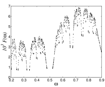
FIG. 1.: Critical function $F_{c}(\omega)$ for $\omega\in[0,1]$ for Hamiltonian (6) with $e=0.45$.

FIG. 2.: Critical threshold $F_{c}$ between $(a)$ resonances 1:1 and 2:1 and $(b)$ resonances 2:1 and 3:1 for co-rotating $(a)$, $(b)$ and counter-rotating $(a)^{\prime}$, $(b)^{\prime}$ orbits. The continuous curves are obtained by renormalization and dashed curves by the 2/3-rule criterion.

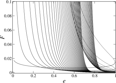
FIG. 3.: Critical threshold $F_{c}$ between various primary resonances $m$:1 and $m$+1:1 for $m=1,\ldots,40$ from left to right, obtained by the 2/3-rule criterion for co-rotating orbits (continuous curves) and counter-rotating orbits (dashed curves).

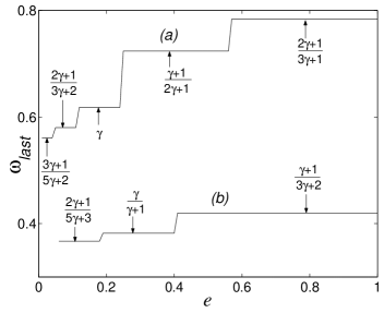
FIG. 4.: Value $\omega_{last}$ of the frequency of the last invariant torus for Hamiltonian (6) as a function of the parameter $e$ : $(a)$ between resonances 1:1 and 2:1, and $(b)$ between resonances 2:1 and 3:1.

REFERENCES

- [1] J.E. Bayfield and P.M. Koch, Phys. Rev. Lett. 33, 258 (1974).
- [2] B.I. Meerson, E.A. Oks, and P.V. Sasorov, JETP Lett. 29, 72 (1979).
- [3] G. Casati, B.V. Chirikov, D.L. Shepelyansky, and I. Guarnieri, Phys. Rep. 154, 77 (1987).
- [4] L.E. Reichl, The Transition to Chaos in Conservative Classical Systems: Quantum Manifestations (Springer-Verlag, New York, 1992).
- [5] B.V. Chirikov, Phys. Rep. 52, 263 (1979).
- [6] A.J. Lichtenberg and M.A. Lieberman, Regular and Chaotic Dynamics (Springer-Verlag, New York, 1992).
- [7] D.F. Escande, Phys. Rep. 121, 165 (1985).
- [8] J.M. Greene, J. Math. Phys. 20, 1183 (1979).
- [9] J. Laskar, Physica D 67, 257 (1993).
- [10] J. Laskar, in Hamiltonian Systems with Three or More Degrees of Freedom, edited by C. Simó, NATO Advanced Study Institute Series C, Vol. 533 (Kluwer Academic, Dordrecht, 1999).
- [11] C. Chandre and H.R. Jauslin, to appear in Physics Reports (2001).
- [12] C. Chandre, M. Govin, H.R. Jauslin, and H. Koch, Phys. Rev. E 57, 6612 (1998).
- [13] C. Chandre and H.R. Jauslin, Phys. Rev. E 61, 1320 (2000).
- [14] C. Chandre, Phys. Rev. E 63, 046201 (2001).
- [15] C. Chandre, J. Laskar, G. Benfatto, and H.R. Jauslin, Physica D 154, 159 (2001).
- [16] A.F. Brunello, T. Uzer, and D. Farrelly, Phys. Rev. A 55, 3730 (1997).
- [17] N.B. Delone, B.P. Krainov, and D.L. Shepelyanski, Sov. Phys. Usp. 26, 551 (1983).
- [18] J.E. Howard, Phys. Rev. A 46, 364 (1992).
- [19] K. Sacha and J. Zakrzewski, Phys. Rev. A 55, 568 (1997).
- [20] H. Koch, Erg. Theor. Dyn. Syst. 19, 475 (1999).
- [21] J.J. Abad and H. Koch, Commun. Math. Phys. 212, 371 (2000).
- [22] M.R.W. Bellermann, P.M. Koch, D.R. Mariani, and D. Richards, Phys. Rev. Lett. 76, 892 (1996).
- [23] E.J. Galvez, B.E. Sauer, L. Moorman, P.M. Koch, and D. Richards, Phys. Rev. Lett. 61, 2011 (1988).
- [24] R.V. Jensen, S.M. Susskind, and M.M. Sanders, Phys. Rev. Lett. 62, 1476 (1989).
- [25] R.S. MacKay, Physica D 33, 240 (1988).