Strong NLS Soliton-Defect Interactions

Abstract

We consider the interaction of a nonlinear Schrödinger soliton with a spatially localized (point) defect in the medium through which it travels. Using numerical simulations, we find parameter regimes under which the soliton may be reflected, transmitted, or captured by the defect. We propose a mechanism of resonant energy transfer to a nonlinear standing wave mode supported by the defect. Extending Forinash et. al. [1], we then derive a finite-dimensional model for the interaction of the soliton with the defect via a collective coordinates method. The resulting system is a three degree-of-freedom Hamiltonian with an additional conserved quantity. We study this system both numerically and using the tools of dynamical systems theory, and find that it exhibits a variety of interesting behaviors, largely determined by the structures of stable and unstable manifolds of special classes of periodic orbits. We use this geometrical understanding to interpret the simulations of the finite-dimensional model, compare them with the nonlinear Schrödinger simulations, and comment on differences due to the finite-dimensional ansatz.

To fit into Arxiv’s file size requirements, low-resolution versions of certain large figures were used. A version of this paper with the full figures is available at

http://m.njit.edu/~goodman/

1 Introduction

In a previous study, involving the first and last authors [2], (Bragg) resonant nonlinear propagation of light through optical waveguides with a periodically varying refractive index profile and localized defects was investigated. In that work, an approach to the design of spatial defects in a periodic structure for the purpose of trapping and localizing light pulses was suggested and explored. The technique involves resonant transfer of energy from traveling waves (gap solitons) to nonlinear standing wave modes localized at the defect. The cubic nonlinear Schrödinger (NLS) equation with localized potentials, which we study in the present paper, provides a simpler model exhibiting similar phenomena that is more amenable to analysis In particular, in numerical simulations of NLS solitons incident on a single delta-well (point) defect in a one-dimensional continuum, we find a variety of behaviors depending on the parameters describing the soliton.

Several studies have examined the propagation of nonlinear waves through variable or random media. The approach taken in [3, 4] is to view such a medium as sequence of individual weak scatterers, each modeled by a repulsive delta function potential barrier. The interaction of a soliton with an individual scatterer is formulated as a mapping of internal soliton parameters; a soliton which interacts weakly with a scatterer adjusts its internal parameters slightly due to radiative loss of energy. The interaction with the full medium is approximated by repeated composition of this simple mapping.

The problem we address is different in a number of respects. We consider strong interactions of a soliton incident on a single scatterer or defect potential. Furthermore, our potential is taken to be an attractive delta function potential well, which has a single localized eigenstate (defect mode). Therefore, an incident soliton can be expected to break up into a soliton with adjusted parameters, due to energy transfer to the localized defect mode, and to outgoing radiation. Components of the soliton’s energy may be reflected by the potential, transmitted through the potential, or captured by its intrinsic modes. These strong nonlinear scattering interactions exhibit a great deal of complexity, which we explore first by direct numerical simulation and then via finite dimensional models.

In particular, we first conduct a series of numerical experiments on the partial differential equation (PDE), in which a variety of of phenomena are observed, which we may partly explain by a resonant transfer of energy to standing wave modes localized at the defect. Second, we derive a finite-dimensional system of ordinary differential equations (ODEs) that models the interaction of solitons with nonlinear standing wave ‘defect’ modes supported by the potential. This part of the analysis is similar in spirit to our earlier study of a finite dimensional reduction of the simpler case of kinks interacting with a trapped mode in the sine-Gordon equation with a point defect [5]. After reviewing the basic PDE model in Section sec:pde and 3, and describing the results of direct numerical simulations in Sections 4, we outline the (formal) finite-dimensional reduction procedure in Section 5. We then describe in Section 6 a representative set of three numerical experiments, in the same parameter ranges as the PDE studies, that reveal the kinds of soliton transmission, reflection and transient capture behaviors that the ODEs exhibit. Section 7 is devoted to analysis of the ODEs. We describe invariant subspaces and special sets of orbits, focusing on the stable and unstable manifolds of certain periodic orbits. These are shown to partially ‘organize’ the global dynamics, in particular providing separatrices between transmitted and reflected soliton orbits. In the final Section 8, we make comparisons between the PDE and ODE dynamics and summarize. Detailed analytical calculations, and some background material, are relegated to an Appendix.

In addition to our specific study of NLS soliton-defect mode interactions, we believe that the detailed comparison of PDE and ODE solutions in this paper has general implications for similar ‘collective coordinate’ finite-dimensional representations commonly used to study dynamical interactions of continuous fields.

2 The nonlinear Schrödinger (NLS) equation with a point defect

We consider a nonlinear Schrödinger (NLS) equation with a spatially localized ‘attractive’ impurity (a defect potential well) at the origin:

$$iu_{t}+\frac{1}{2}u_{xx}+\lvert u\rvert^{2}u+\gamma\;\delta(x)u=0,\ \ \gamma>0.$$ (2.1)

In the absence of a defect ($\gamma=0$), this system supports a two-parameter family of solitons of the form

$$u_{\rm{Sol}}(x,t)=\eta\operatorname{sech}(\eta(x-vt))e^{i(vx-\omega t)},$$ (2.2)

where $\omega=-\frac{1}{2}(\eta^{2}-v^{2})$ is the temporal frequency. Solitons are nonlinear bound states which play a fundamental role in the unperturbed ($\gamma=0$) NLS equation, and we are especially interested in their behavior in the perturbed system. For $\gamma>0$, (2.2) does not solve (2.1), but far from the defect, the soliton propagates essentially without distortion and at constant speed $v$ due to the exponentially small overlap of soliton and potential.

Equation (2.1) also supports exact nonlinear bound state or defect mode solutions of the form

$$u_{\rm{Def}}(x,t)=ae^{ia^{2}t/2}\operatorname{sech}{(a\lvert x\rvert+\tanh^{-1}\frac{\gamma}{a})},$$ (2.3)

for all $a\geq\gamma$. These solutions are constructed from a stationary ($v=0$) soliton on each side of the defect pasted together at $x=0$ to satisfy the conditions of continuity at $x=0$ and the appropriate jump condition in the first derivative at $x=0$, $u(0^{+})-u(0^{-})=-2\gamma u(0)$. For both bound state families, $u_{\rm Sol}$ and $u_{\rm Def}$, the frequency of oscillation depends nonlinearly on its amplitude.

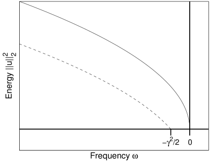
Figure 2.1: The frequency and amplitude of a soliton in the absence of a defect (solid), and of the defect mode (dashed).

The chief concern of this paper is to understand strong interactions between solitons and the delta well defect. If the defect strength $\gamma$ is small of the soliton velocity is large, then the interaction is weak: a small amount of energy is lost to radiation, and the soliton continues past the defect with minor changes to the parameters that define it. In the case of weak interactions, estimates for the energy loss of the soliton can be obtained by the first order perturbation theory (the Born approximation) [4, 3]. When $\gamma$ is sufficiently large and $v$ is small, stronger interactions can take place, the character of which may be understood in terms of a nonlinear resonance that in some cases takes place between the soliton and the defect mode.

Solitons with $v=0$ have $\|u_{\rm{Sol}}\|_{L^{2}}^{2}=2\eta$ and frequency $-\eta^{2}/2$, whereas nonlinear defect modes have $\|u_{\rm{Def}}\|_{L^{2}}^{2}=2(a-\gamma)$ and frequency $-a^{2}/2$. In Figure 2.1 we plot the squared $L^{2}$ norm of these two types of mode as functions of frequency. In the following section we discuss the bifurcation diagram of Figure 2.1 and its implications, and review the well-posedness theory of the initial value problem and the dynamic stability theory for $u_{\rm Sol}$ and $u_{\rm Def}$. Due to the relation between the square of the $L^{2}$ norm with the electromagnetic energy in the context of optics, we shall refer to $\|u_{\rm{Sol}}\|_{L^{2}}^{2}$ and $\|u_{\rm{Def}}\|_{L^{2}}^{2}$ as the energy of the soliton and defect modes, and more generally to the square of the $L^{2}$ norm of $u$ over a region of space as the energy contained in that region.

Note that no defect modes exist in the frequency range $\omega\in(-\gamma^{2}/2,0]$. This observation is crucial in predicting which solitons will be trapped and which reflected by the potential. We find, roughly, that sufficiently slow solitons with $\eta>\gamma$ are trapped upon encountering the defect, while slow solitons with $\eta<\gamma$ are reflected by the defect. This suggests that trapping occurs via resonant energy transfer from the soliton to the defect mode. If the incoming soliton has frequency less than $-\gamma^{2}/2$, it can and may excite a nonlinear defect mode and transfer its energy to that mode. Otherwise, as in [6], we find that the defect behaves as a scatterer, splitting the incoming wave into transmitted, captured, and reflected parts. This behavior differs sharply from one seen in nonlinear optics: in the nonlinear coupled mode equations describing the interaction of gap solitons with nonlinear defect modes [2], it was found that in the absence of resonance, pulses were either coherently reflected or transmitted after interacting with the defect, with little energy captured or lost to radiation.

3 Overview of well-posedness and stability

Structural properties of NLS:  The nonlinear Schrödinger equation (2.1) is a Hamiltonian system, which can be written in the form:

$$iu_{t}\ =\ \frac{\delta}{\delta u^{*}}{\mathcal{H}}[u,u^{*}],\$$ (3.1)

where ${\mathcal{H}}[u,u^{*}]$ denotes the Hamiltonian:

$${\mathcal{H}}[u,u^{*}]\ =\ \int\ \left(\ \frac{1}{2}|u_{x}|^{2}\ -\ \frac{1}{2}|u|^{4}\ -\ \gamma\delta(x)|u|^{2}\ \right)\ dx$$

$$=\ \int\ \left(\ \frac{1}{2}|u_{x}|^{2}\ -\ \frac{1}{2}|u|^{4}\ \right)\ dx-\ \gamma|u(0)|^{2}\ .$$ (3.2)

Invariance with respect to time-translations implies that ${\mathcal{H}}[u,u^{*}]$ is conserved by the flow generated by (3.1). Additionally, invariance under the transformation $u\mapsto e^{i\xi}u,\ \xi\in R^{1}$ implies that

$${\mathcal{N}}[u,u^{*}]\ =\ \int|u|^{2}\ dx=\ ||u||_{2}^{2}$$ (3.3)

is a conserved integral.

For the spatially translation invariant case, $\gamma=0$, NLS has the Galilean invariance:

$$u(x,t)\ \mapsto\ u(x-vt,t)\ e^{i(xv-\frac{1}{2}v^{2}t)},\ v\in R^{1}.$$ (3.4)

Well-posedness theory: The functionals ${\mathcal{H}}[\cdot]$ and ${\mathcal{N}}[\cdot]$ are well defined on $H^{1}(R^{1})$, the space of functions $f$, for which $f$ and $\partial_{x}f$ are square integrable. It is therefore natural to construct the flow for initial data of class $H^{1}$. In fact, it can be shown that, for initial conditions $u_{0}=u(x,t=0)\in H^{1}(R^{1})$, there exists a unique global solution of NLS, $u\in C^{0}(R^{1};H^{1}(R))$, in the sense of the equivalent integral equation:

$$u(t)\ =\ U(t)u_{0}\ +i\int_{0}^{t}U(t-s)\ |u(s)|^{2}u(s)\ ds,$$ (3.5a)

$$U(t)\ \equiv\ \exp\left(-iHt\right),\ H\equiv-\frac{1}{2}\partial_{x}^{2}-\gamma\delta(x).$$ (3.5b)

The spectral decomposition of $H$ is known explicitly [7] and can be used to construct $U(t)$ explicitly.

To show the existence of a solution to (3.5a) in $H^{1}$, we must show the existence of a $C^{0}(R^{1};H^{1}(R))$ fixed point of the mapping $u(x,t)\mapsto J[u](x,t)$, given by the right hand side of (3.5a).

We now outline the key ingredients of the proof. To bound $J[u]$ and its first derivative in $L^{2}$, we introduce the operator ${\mathcal{A}}=I+P_{c}H$, where $P_{c}$ denotes the projection onto the continuous spectral part of $H$. Note that ${\mathcal{A}}$ is a nonnegative operator, since the continuous spectrum of $H$ is the nonnegative real half-line. Moreover, we expect $\|{\mathcal{A}}^{\frac{1}{2}}f\|\ \sim\|f\|_{H^{1}}\equiv\ \|(I-\partial_{x}^{2})^{\frac{1}{2}}f\|_{L^{2}}$. In fact, we shall use that the following operators are bounded from $L^{2}$ to $L^{2}$:

$${\mathcal{A}}^{\frac{1}{2}}(I-\partial_{x}^{2})^{-\frac{1}{2}},\ {\mathcal{A}}^{\frac{-1}{2}}(I-\partial_{x}^{2})^{\frac{1}{2}}.$$

This follows from the boundedness of the wave operators on $H^{1}$ [8]. Therefore, we have an equivalence of norms

$$C_{1}\ \|f\|_{H^{1}}\ \leq\ \|{\mathcal{A}}^{\frac{1}{2}}f\|_{L^{2}}\ \leq\ C_{2}\ \|f\|_{H^{1}}.$$ (3.6)

Our formulation (3.5a) and introduction of ${\mathcal{A}}$ is related to the nice property that ${\mathcal{A}}$, and hence also functions of ${\mathcal{A}}$, commute with the propagator $\exp(-iHt)$. We shall also use the Sobolev inequality:

$$|f(x)|^{2}\leq\ C\|f\|_{L^{2}}\|\partial_{x}f\|_{L^{2}},$$ (3.7)

and the Leibniz rule [9]:

$$\|(I-\partial_{x}^{2})^{\frac{1}{2}}(fg)\|\ \leq\ C\left(\|f\|_{L^{\infty}}\ \|(I-\partial_{x}^{2})^{\frac{1}{2}}g\|_{L^{2}}\ +\ \|(I-\partial_{x}^{2})^{\frac{1}{2}}f\|_{L^{2}}\ \|g\|_{L^{\infty}}\right).$$ (3.8)

Since $U(t)$ is unitary in $L^{2}$, we have

$$\|{\mathcal{A}}^{\frac{1}{2}}J[u]\|_{L^{2}}\$$

$$\leq\ \|{\mathcal{A}}^{\frac{1}{2}}u_{0}\|_{L^{2}}\ +\ \gamma\int_{0}^{t}\|{\mathcal{A}}^{\frac{1}{2}}|u(s)|^{2}u(s)\|_{L^{2}}\ ds$$

$$=\ \|{\mathcal{A}}^{\frac{1}{2}}u_{0}\|_{L^{2}}\ +\ \gamma\int_{0}^{t}\|\left({\mathcal{A}}^{\frac{1}{2}}(I-\partial_{x}^{2})^{-\frac{1}{2}}\right)\cdot\left((I-\partial_{x}^{2})^{\frac{1}{2}}|u(s)|^{2}u(s)\right)\|_{L^{2}}\ ds.$$ (3.9)

By (3.6)), (3.7), and (3.8),

$$\|J[u](t)\|_{H^{1}}\ \leq\ C\|{\mathcal{A}}J[u]\|_{L^{2}}\ \leq\ C_{1}\|u_{0}\|_{H^{1}}\ +\ C_{2}\ T\ \sup_{s\in[0,T]}\|u(s)\|_{H^{1}}^{3}.$$ (3.10)

Now assume that $u$ is such that $\sup_{s\in[0,T]}\|u(s)\|_{H^{1}}\leq 2C_{1}$. Then, by (3.10), by choosing $T<T_{1}$ sufficiently small. $\sup_{s\in[0,T]}\|J[u](s)\|_{H^{1}}\leq 2C_{1}\|u_{0}\|_{H^{1}}$.

$$\|J[u](t)\|_{H^{1}}\ \leq\ C_{1}\|u_{0}\|_{H^{1}}\ +\ C_{2}\ T\ \left(2C_{1}\|u_{0}\|_{H^{1}}\right)^{3}.$$

It follows that for $0<T<T_{1}$ sufficiently small, the transformation $J[\cdot]$ maps a ball $C^{0}([0,T];H^{1}(R))$ into itself. A similar calculation shows that

$$\|J[u](t)\ -\ J[v](t)\|_{H^{1}}\ \leq\ K\ T\ \left(2C_{1}\|u_{0}\|_{H^{1}}\right)^{2}\ \sup_{s\in[0,T]}\ \|u(s)-v(s)\|_{H^{1}},$$ (3.11)

and therefore for $0<T<T_{2}\leq T_{1}$, the transformation $J[\cdot]$ is a contraction on this ball. Therefore, $J[\cdot]$ has a unique fixed point in $C^{0}([0,T];H^{1}(R))$ for $T$ sufficiently small and local existence in time of the flow follows. Global existence in time follows from the á priori bound on the $H^{1}$ norm of the solution implied by the time-invariance of $L^{2}$ norm and Hamiltonian.

Nonlinear bound states: Bound states are an important class of solutions having the form:

$$u_{b}(x,t)\ =\ e^{-i\lambda t}\varphi(x;\lambda),\ \varphi\in L^{2}.$$ (3.12)

For the linear Schrödinger equation, the functions $\varphi$ are eigenstates of a Schrödinger operator: $-\frac{1}{2}\partial_{x}^{2}-\gamma\delta(x)$ and satisfy the equation

$$-\frac{1}{2}\varphi_{xx}\ -\ \gamma\delta(x)\varphi=\lambda\varphi.$$ (3.13)

Bound states are known to play a fundamental role in the general dynamics of the linear Schrödinger equation. This is a consequence of the spectral decomposition of linear self-adjoint operators.

For NLS, such bound states satisfy the equation:

$$-\frac{1}{2}\varphi_{xx}\ -\ \left(\ \gamma\delta(x)\ +\ |\varphi|^{2}\ \right)\varphi\ =\ \lambda\varphi,$$ (3.14)

and have the general character of ‘nonlinear eigenstates’, although there is no rigorous decomposition theory of solutions into such states, except in the completely integrable case $\gamma=0$ [10]. For this translation-invariant case there is family of solitary traveling wave solutions (2.2). These are Galilean boosts of the basic solitary standing wave (2.2) with $v=0$; see (3.4). For $\gamma>0$, the equation is no longer translation-invariant and we have the defect or ‘pinned’ states of (2.3). These two families of nonlinear bound states are plotted in bifurcation diagram of Figure 2.1. We note that for $\gamma=0$ the family of solitons bifurcates from the zero state at zero frequency, the endpoint of the continuous spectrum of the linearized operator $-\partial_{x}^{2}$ about the zero state. For $\gamma>0$, the family of defect states bifurcates from the zero state in the direction of the eigenfunction of the linearized operator, $-\partial_{x}^{2}-\gamma\delta(x)$, and at the corresponding eigenfrequency $\lambda=-\gamma^{2}/2$; see [11] for a general discussion.

Stability of nonlinear bound states: An alternative characterization of the nonlinear bound states $u_{\rm Sol}$ and $u_{\rm Def}$ is variational. The advantage of the variational characterization is that it can be used to establish nonlinear stability of the ‘ground state; see [12, 11].

Theorem 1

(I) The families of nonlinear bound state profiles $\eta\mapsto\varphi_{Sol}(x;\eta)$ for the case $\gamma=0$ and $a\mapsto\varphi_{Def}(x;a)$ for the case $\gamma>0$ can be characterized variationally as minimizers of the Hamiltonian, ${\mathcal{H}}$, subject to fixed $L^{2}$ norm, ${\mathcal{N}}$:

$$\min_{\varphi}\ {\mathcal{H}}[\varphi],\ \ {\mathcal{N}}[\varphi]=\rho$$ (3.15)

Thus $u_{\rm Sol}$ and $u_{\rm Def}$ are called ground states in their respective cases. Their associated frequencies, $\lambda(\rho)=-\eta^{2}/2$ and $\lambda(\rho)=-a^{2}/2$ arise as Lagrange multipliers for the constrained variational problem (3.15). As $\rho\to 0$, $\lambda(\rho)\to 0$, respectively, $\lambda(\rho)\to-\gamma^{2}/2$.

(II) Ground states are $H^{1}$ nonlinearly orbitally Lyapunov stable, i.e. if the initial data are $H^{1}$ close to a soliton (modulo the NLS symmetries), then the solution remains close to a soliton in this sense for all $t\in(-\infty,\infty)$.

For results on asymptotic stability of nonlinear ground states, see [13, 14, 15, 16, 17].

High energy defect modes and solitons: Solitons of the translation-invariant NLS equation ($u_{\rm Sol}$ of (2.2) for $\gamma=0$) may be related to the high energy ($L^{2}$ norm) nonlinear bound states, $u_{\rm Def}$, in an appropriate limit. The following summary is based on the variational principle of Theorem 1, and does not require the explicit formula (2.3) for the defect mode. This argument can also be applied to more general linear potentials $V(x)|u|^{2}$ in the Hamiltonian in place of $\delta(x)|u|^{2}$, and to more general nonlinearities.

Consider the variational problem (3.15), in which we make explicit the dependence of the Hamiltonian ${\mathcal{H}}$ on the defect strength $\gamma$ by writing ${\mathcal{H}}(u;\gamma)$ in place of the notation of (3.2). Define $T_{\rho}[u](x)=\rho u(\rho x)$, for $\rho>0$. Then, $\frac{1}{\rho^{3}}{\mathcal{H}}(T_{\rho}[u];\gamma)={\mathcal{H}}(u;\frac{\gamma}{\rho})$. If ${\mathcal{I}}(\rho;\gamma)$ denotes the minimum in (3.15), we therefore have:

$$\frac{1}{\rho^{3}}{\mathcal{I}}(\rho;\gamma)={\mathcal{I}}(1;\frac{\gamma}{\rho}).$$

Note that, as $\rho\to\infty$, ${\mathcal{I}}(1;\frac{\gamma}{\rho})$ formally approaches ${\mathcal{I}}(1;0)$, the constrained minimum of the cubic NLS Hamiltonian ${\mathcal{H}}(u;0)$, and that the extremizer is the classical one-soliton. It can be shown that if $u_{\rm Def}(x;a)$ denotes the nonlinear defect mode and we define $U_{D}$ by $T_{1/a}[u_{\rm Def}](x;a)=U_{D}(x;a)$, then $U_{D}(x;a)$ converges strongly to the classical one-soliton of norm one. It follows that, for large $a$, $u_{\rm Def}(x,a)$ looks more and more like a $T_{a}$-scaled soliton (a solitary standing wave) of the translation-invariant NLS.

4 Direct Numerical Simulations of the PDE

In this section we discuss simulations of the initial value problem for the NLS equation (2.1). All numerical experiments in this section were performed using a modification of a finite difference approximation due to Fei, Pérez-García and Vázquez [18], which conserves a discrete $L^{2}$ norm and, in the absence of a defect, a discrete analog of the Hamiltonian. The method is accurate to second order in both space and time, and is implicit only in its linear terms. Therefore, it requires a linear equation to be solved at each step. The Dirac delta function is approximated either as a single point discontinuity, or by a smoother function with very small support, with similar results in either case.

In the numerical experiments, a soliton is initialized far from the defect with prescribed velocity $v$ and amplitude $\eta$ and is allowed to propagate toward the defect location. A wide variety of behaviors is seen as parameters are varied. For simplicity (and motivated by a scaling argument given in section 5) we limit our study to defects with strength $\gamma=1$. Therefore, the branch of nonlinear defect modes bifurcates at the frequency $-1/2$. The nonlinear resonance summarized in Figure 2.1 is useful in understanding the various behaviors that are possible in this interaction. In the figures that follow, $|u|$ is plotted although the system’s $L^{2}$ conservation might suggest plotting $|u|^{2}$. This is done to render visible the radiation that is shed during the interaction.

In the first set of runs, $\eta$ is set to 4, and $v$ is varied between 1 and 2. In this case, the solution remains mainly soliton-like, with very little loss of energy to radiative modes. There exists a critical velocity, above which the soliton is transmitted past the defect, although with diminished speed, and below which the soliton transfers its energy to a nonlinear defect mode. Figure 4.1 shows the input versus output velocities, indicating the critical velocity $v_{c}\approx 1.78$. Figure 4.2 shows the evolution of $|u(x,t)|$ up to a time somewhat after the interaction has taken place. In the left hand figure, the initial velocity was about $v=1.65$, and after some time the solution is a defect mode centered at $x=0$ with a small amount of radiation. In the right hand figure, with initial velocity greater than $v_{c}$, the soliton largely survives, although some of the incoming soliton’s energy is captured by the defect and, as time proceeds, eventually takes on the form of a small amplitude defect mode.

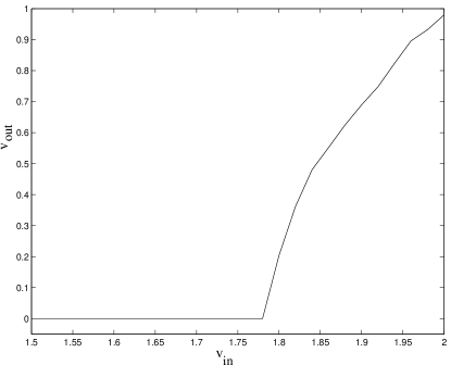
Figure 4.1: Input versus output velocities of a soliton with $\eta=4$.

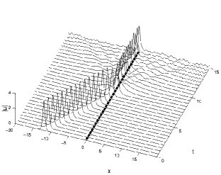
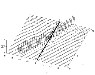
Figure 4.2: The soliton amplitude $|u|$ after interaction with the soliton, with large initial soliton amplitude $\eta=4$. On the left, a slower soliton is captured. On the right, a faster soliton is transmitted, leaving behind a small defect mode. The transition from capture to transmission is abrupt, occurring at a critical velocity $v_{c}\approx 1.78$, as seen in Figure 4.1.

When $\eta$ is reduced to 2, the behavior changes. The simulations show a more complicated nonlinear scattering process. The pulse splits into three parts: reflected, captured, and transmitted. In all cases, a significant defect mode is created. The faster the soliton’s initial speed, the smaller the defect mode remaining in a neighborhood of the origin and the larger the transmitted portion. An example is shown in Figure 4.3 and the phenomenon is summarized in Figure 4.4, which shows how the fraction of energy deposited into the defect mode decays monotonically as the input velocity increases.

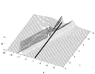
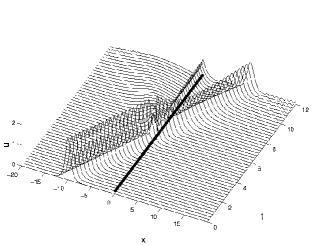
Figure 4.3: A soliton with initial amplitude $\eta=2$ has a large amount of its energy captured by the defect. At left, a slower soliton with $v=1.5$ has a substantial portion of its energy captured. At right, as the incoming soliton’s velocity is increased to $v=1.75$ , less energy is captured and a larger soliton gets through.

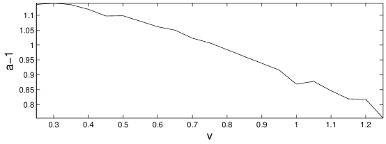
Figure 4.4: For $\eta=2$, as the input velocity is increased, the total amount of energy captured by the defect mode decreases.

When $\eta$ is further decreased to $0.5$, the behavior alters yet again. In this case, only a small amount of energy is captured by the defect, while large amounts are reflected and transmitted; see Figure 4.5. When the incoming velocity is sufficiently small, the soliton appears to be completely reflected and when the incoming velocity is sufficiently large, the soliton is nearly completely transmitted. For intermediate velocities, the pulse is split into a transmitted and a reflected wave. This nonlinear scattering phenomenon is studied by Cao and Malomed [6], who derive approximate reflection and transmission coefficients for the interaction in the case of small $\eta$.

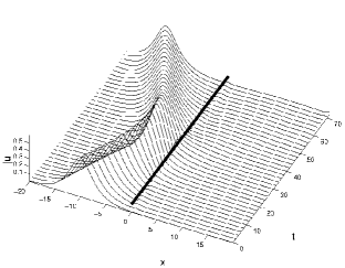
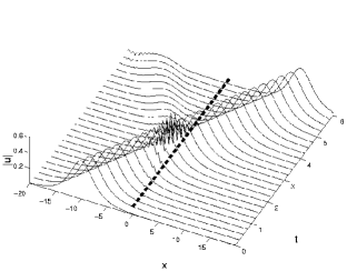
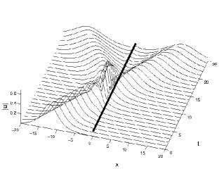
Figure 4.5: When $\eta=0.5$, most of the wave is reflected with $v=0.25$ (left) or transmitted when $v=4$ (right). When $v=1$, the wave is split nearly in half into reflected and transmitted portions.

4.1 Discussion of Simulations

We wish to interpret the scattering of solitons by defects in terms of the amplitude-frequency curves of Figure 2.1. In the previous section, as the soliton amplitude parameter $\eta$ is decreased, two effects make the transfer of energy from the soliton to the defect mode less efficient and enhance the scattering. At first, for $\eta=2$, the amount of $L^{2}$ energy lost in the interaction is increased, compared to the experiments with $\eta=4$. Finally, for $\eta<\gamma$, there no longer exists a nonlinear defect mode that resonates with the incoming soliton, and therefore almost no energy is captured.

It was suggested in [2], in the context of the nonlinear coupled mode equations, that for sufficiently slow incident solitons, a simple resonant energy transfer mechanism should hold. In particular, a good approximate predictor of the distribution of trapped energy would be given by the vertical projection of the point corresponding to the incident soliton onto the corresponding point on the defect mode curve with the same frequency. It turns out that this approximation is valid in certain cases, but extensive further simulations have shown the general situation to be more complicated. In this subsection we explore this issue by means of the following auxiliary numerical experiment.

We initialized a family of solitons with zero velocity and varying amplitudes $\eta$, centered directly over the defect, and let them run forward until they formed standing wave states (recall that the defect standing wave (2.3) is an exact solution of (2.1)). The solutions rapidly evolved into a combination of nonlinear defect modes and radiation. If the above picture applied, then the defect modes thus produced should have almost the same frequencies as the initial solitons. An example is shown in Figure 4.6, which was initialized with $\eta=1$ and $\gamma=1$. Figure 4.7 reproduces the two curves of Figure 2.1 with arrows connecting each soliton’s initial conditions to the periodic solution of the corresponding defect mode following the interaction. The arrows are far from vertical, and show a consistent downward frequency shift. Evidently, in this experiment the above ‘direct’ resonant exchange mechanism does not apply.

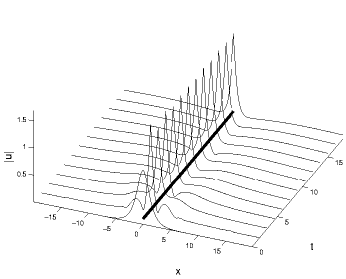
Figure 4.6: A soliton initialized over a defect quickly decomposes into a defect mode plus radiation.

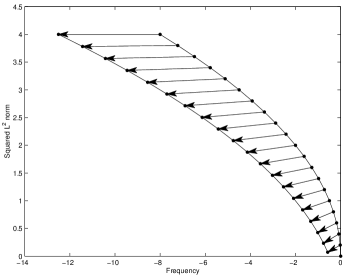
Figure 4.7: Arrows connect soliton initial conditions to defect mode steady periodic solutions.

However, this finding does not contradict the role of resonant energy transfer in trapping an incoming soliton. In the above experiment, in which the ‘incident’ soliton has velocity $v=0$, the mechanism differs from that involving a moving soliton. Were the nonlinear term absent, the results of this auxiliary experiment would be well-understood. Spectral theory dictates that the initial condition decomposes into a bound state and radiative modes, and there is no role in this interaction for the soliton’s internal frequency. In the presence of nonlinearity, the behavior is essentially the same, although we can no longer compute the captured solution as the projection of the initial conditions onto the bound state. The frequency is shifted because the solution is in some sense finding the nonlinear projection of the initial condition onto the family of nonlinear defect modes (2.3), which has only a slightly smaller $L^{2}$ norm. As $a$ is increased, the energy ($L^{2}$ norm) is increased and, as discussed at the end of section 3, the ground state defect mode approaches a scaled one-soliton centered at $x=0$.

By contrast, in the numerical simulations of moving solitons, the defect mode is initially forced by the tail at the soliton’s leading edge, for which the soliton’s internal frequency is important. The defect mode may grow by resonantly extracting energy from the tail, before the bulk of the soliton even reaches the defect. Consequently, when the soliton reaches the defect, the defect mode is large enough that the two modes may interact, and energy may flow from one mode to the other. In the next section, we introduce an ordinary differential equation model of this interaction.

5 A model of soliton-defect interactions

Forinash, Peyrard, and Malomed [1] studied the interaction of a soliton with a linear defect mode using a collective coordinate ansatz to derive a set of approximate equations to describe the evolution of a finite set of variables that characterize the two modes. Their model yielded a complicated set of differential-algebraic equations which was difficult to understand analytically. Here we modify and slightly simplify their ansatz. In particular, we approximate the solution, $u$, as the sum of a time-modulated soliton and a time-modulated nonlinear defect state:

$$u\ =\ u_{\rm{S}}(x;\eta,Z,V,\phi)+u_{\rm{D}}(x;a,\phi,\psi),$$ (5.1)

where $u_{\rm{S}}$ is a generalized soliton of the form

$$u_{\rm{S}}=\eta\operatorname{sech}(\eta x-Z)\;e^{i(Vx-\phi)},$$ (5.2)

and $u_{\rm{D}}$ is a generalized bound state of the form

$$u_{\rm{D}}=a\operatorname{sech}{\left(a\lvert x\rvert+\tanh^{-1}\frac{\gamma}{a}\right)}\;e^{-i(\phi+\psi)}.$$ (5.3)

In (5.2, 5.3), the variables $\eta$, $Z$, $V$, $\phi$, $a$, and $\psi$ are all allowed to depend on $t$. Note that $\rVert u_{S}\rVert^{2}_{L^{2}}=2\eta$ and $\rVert u_{D}\rVert^{2}_{L^{2}}=2(a-\gamma)$. The Lagrangian functional of the NLS equation is evaluated at $u$ (by integrating over the spatial domain), and the resulting function is then interpreted as an effective finite-dimensional Lagrangian whose Euler-Lagrange equations determine the evolution of these variables. Instead of seeking stationary configuations of the (true) Lagrangian with respect to admissible variations of the field variable $u(x,t)$, we consider only variations of the type allowed by the time-dependent variables of the ansatz. This technique, often known as the collective coordinate or variational method, has a long history and is well summarized in a recent survey by Malomed [19].

The NLS Lagrangian (cf. (3.2)) is

$${\mathcal{L}}=\int_{-\infty}^{\infty}\frac{i}{2}(u^{*}u_{t}-uu^{*}_{t})-\frac{1}{2}\lvert u_{x}\rvert^{2}+\frac{1}{2}\lvert u\rvert^{4}+\gamma\delta(x)\lvert u\rvert^{2}dx.$$

We evaluate this integral for our ansatz (5.1-5.3). Unlike [1] and most other analyses of this type of which we are aware, we do not assume that $a$ is small, and we include high-order terms involving $a$. We do make the simplifying assumption that all interaction between the modes $u_{\rm{S}}$ and $u_{\rm{D}}$ takes place through terms involving the delta function. This is, in part, justified because the other interaction terms involve oscillatory integrals which will average out to be much smaller than the terms retained. The resulting effective Lagrangian is given by

$${\mathcal{L}}_{\rm eff}=2\eta\dot{\phi}-2Z\dot{V}+2(a-\gamma)(\dot{\phi}+\dot{\psi})+\frac{1}{3}\eta^{3}-\eta V^{2}+\frac{1}{3}a^{3}+\gamma\eta^{2}\operatorname{sech}^{2}{Z}\\ +2\gamma\eta\sqrt{a^{2}-\gamma^{2}}\operatorname{sech}{Z}\cos{\psi}.$$ (5.4)

This Lagrangian has an associated Hamiltonian, conserved by the Euler-Lagrange (and Hamilton’s) equations:

$$H=-\frac{1}{3}\eta^{3}+\eta V^{2}-\frac{1}{3}a^{3}-\gamma\eta^{2}\operatorname{sech}^{2}{Z}-2\gamma\eta\sqrt{a^{2}-\gamma^{2}}\operatorname{sech}{Z}\cos{\psi}.$$ (5.5)

Since the Hamiltonian is independent of $\phi$, its conjugate momentum

$$p_{\phi}=\frac{\partial{\mathcal{L}}_{\rm eff}}{\partial\dot{\phi}}=2\eta+2(a-\gamma)$$ (5.6)

is conserved by Noether’s theorem [20]. Notice that $p_{\phi}=\rVert u_{S}\rVert^{2}_{L^{2}}+\rVert u_{D}\rVert^{2}_{L^{2}}$. This conservation law is the analogue of the $L^{2}$ conservation law for NLS, (3.3). The phase space of this three degree-of-freedom system can be therefore be expressed as the cross product of the reduced 4-dimensional $(Z,V,a,\psi)$-phase space and the 2-dimensional $(\eta,\phi)$-phase space, with trivial dynamics on the latter, determined from the reduced system via (5.6) and a quadrature (cf. (5.9-5.10) below). In the analysis that follows, we may therefore regard the constant of motion

$$c=\eta(t)+a(t)\ \ (\geq\gamma)$$ (5.7)

as a parameter determined by the initial conditions, and study evolution on the reduced $(Z,V,\psi,a)$-space. Here and henceforth $c$ denotes this constant, and should not be confused with its conventional usage to denote the speed of light.

We note further that the resulting equations are invariant under the rescaling $a\mapsto\gamma a,\;c\mapsto\gamma c,\;t\mapsto t/\gamma^{2}$: implying that, without loss of generality, the parameter $\gamma$ may be set to equal to one. This symmetry belongs only to the reduced system of ODEs, not to the original NLS equation (2.1), but motivates our decision to perform simulations only with $\gamma=1$. Then $c$ is the only parameter remaining in the evolution equations, and these equations are in fact canonically Hamiltonian for the ‘scaled’ Hamiltonian $H/2$, with $H$ of (5.5) written in the Lagrangian coordinates:

$$H=-\frac{c^{3}}{3}+(c-a)\left(ca+V^{2}-(c-a)\operatorname{sech}^{2}Z\right)-2(c-a)\sqrt{a^{2}-1}\operatorname{sech}Z\cos\psi.$$ (5.8)

The final reduced equations, to be studied in Section 7 below, are now:

$$\dot{Z} =(c-a)V,$$ (5.9a)

$$\dot{V} =-(c-a)^{2}\operatorname{sech}^{2}{Z}\tanh{Z}-(c-a)\sqrt{a^{2}-1}\operatorname{sech}{Z}\tanh{Z}\cos{\psi},$$ (5.9b)

$$\dot{\psi} =\frac{c^{2}-2ca-V^{2}}{2}+(c-a)\operatorname{sech}^{2}{Z}+\frac{(2a^{2}-ca-1)}{\sqrt{a^{2}-1}}\operatorname{sech}{Z}\cos{\psi},$$ (5.9c)

$$\dot{a} =-(c-a)\sqrt{a^{2}-1}\operatorname{sech}{Z}\sin{\psi},$$ (5.9d)

with $\phi$ evolving according to:

$$\dot{\phi}=-\frac{(c-a)^{2}-V^{2}}{2}-(c-a)\operatorname{sech}^{2}{Z}-\sqrt{a^{2}-1}\operatorname{sech}{Z}\cos{\psi}.$$ (5.10)

Before analyzing these ODEs, we describe numerical experiments that reveal interesting interactions between the soliton and the defect mode, and suggest specific questions.

6 ODE Simulations of the initial value problem

We now describe a set of numerical experiments for the ODE (5.9) analogous to those discussed in Section 4 for the PDE. We initialize a soliton at $Z(0)=-Z_{0}$ with $|Z_{0}|\gg 1$, set equal to 20 for these simulations. The velocity parameter is set to $V(0)=V_{\rm in}$, propagating rightward toward the defect. For subsequent comparison with the PDE simulations, we note that the variable $V$ in (5.9) is related to the soliton velocity $v$ of (2.2) via $v=\eta V$ by (5.9a) and (5.7). The soliton amplitude is set to $\eta(0)=\eta_{0}$, and we assume there is no energy initially in the defect mode, so $a(0)=\gamma=1$. Thus the relation (5.7) fixes the constant $c$. (Because of the singularity of Equation (5.9c), we set $a(0)=1+\varepsilon$, where $\varepsilon\ll 1$; values between $\varepsilon=10^{-8}$ and $\varepsilon=10^{-5}$ were used in these computations. For some of the effects seen, $\varepsilon$ needs to be set to the small end of this range to get stable results, due to the singularity in (5.9c). ) Finally, we set $\psi(0)=0$. Note that, for large $|Z|$, the $\psi$ dependence becomes exponentially weak, so we do not expect strong $\psi$-dependent effects.

We choose a representative set of $\eta(0)$, or equivalently, $c$ values. For each fixed $\eta(0)$ we allow $V_{\rm in}$ to vary over a range of values, and numerically integrate (5.9) until the soliton center, $Z(t)$, reaches the defect ($Z(t)\sim 0$), (eventually) exits the defect region, and reaches $Z=+Z_{0}$ or $Z=-Z_{0}$ at, say $t=T$. By a variant of the Poincaré recurrence theorem, as in [5], we can show that the soliton must eventually escape any bounded set containing the defect; cf. Section 7.1 below. We then plot the soliton’s outgoing velocity parameter $V_{\rm out}$ (related to the physical velocity by (5.9a)), and the amplitude $(a(T)-1)$ of the defect mode as functions of $V_{\rm in}$. For $Z_{0}$ sufficiently large and $\varepsilon$ sufficiently small, the initial value of the phase difference $\psi$ was indeed found to be unimportant in determining the values of $V(T)$ and $(a(T)-1)$. In interpreting these results, it is important to realize that the dynamics takes place in four-dimensional phase space, and that the figures merely show projections of trajectories on lower dimensional subspaces.

6.1 Experiment 1: large $\eta$.

We observe several distinct types of behavior. The behavior for $\eta=4$ is shown in Figure 6.1. In this case we find a sharp change in behavior at a critical velocity parameter $V_{c}\approx 0.55$. Above this velocity, solitons pass through the defect without significant interaction, merely decreasing their velocities and transferring a little energy to the defect mode. Below $V_{c}$, however, the soliton interacts with the defect, oscillating within the defect region a finite and apparently random number of times before being ejected either to the right or the left. It is also striking that the amount of energy remaining in the defect mode seems to be restricted to two levels: either $a-1\approx 3$ or $a-1\ll 1$. This behavior is apparently governed by the structure of the invariant manifolds of degenerate fixed points at $|Z|=\infty$. Since there exist solutions to (5.9) with $Z$ bounded, as well as solutions which approach $Z=\infty$ with $V>0$, these must be separated by solutions for which $Z\to\infty$ while $V\to 0$. Along with the apparantly arbitrarily fine structure of transmission and reflection zones, Figure 6.1 further shows wide reflection windows of the type reported in many previous studies, e.g. [21, 22, 23, 24].

In Section 7.1 we will investigate the stable and unstable manifolds that are responsible for this behavior, but we give a brief preview here. Figure 6.2 shows the $(Z,V)$ projections of trajectories with nearby initial velocities on either side of $V_{c}$ ($V(0)=V_{c}\pm.002$). The solid curve comes close to an orbit apparently asymptotic to $(Z,V)=(\infty,0)$, and then turns back and is transiently captured before eventual reflection, while the dashed curve approaches infinity with $V$ bounded above zero, and is transmitted without further interaction. This ‘separatrix’ behavior is repeated in the multiple transmission and reflection windows for $V<V_{c}$ (Figure 6.1) and is reminiscent of that found in our earlier study of an ODE model of kink-defect interaction in the sine-Gordon equation [5], and shown there to be related to the homoclinic tangle formed by transverse intersection of stable and unstable manifolds of periodic orbits at $|Z|=\infty$: compare Figure 6.1 with Figure 3.2 of [5].

The ODEs’ behavior should be compared with the direct numerical simulations of solitons with $\eta=4$, as shown in Figure 4.1. The critical velocity is overestimated by $24\%$ ($v_{c}=\eta V_{c}=2.21$ cf. $1.78$ for the PDE), and the PDE simulations show no evidence of the fine structure of transmission and reflection zones below $v_{c}$. This difference, partially due to neglect of radiation damping in the ODEs, is discussed in section 8.

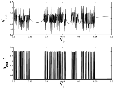
Figure 6.1: (Top) Outgoing velocity vs. incoming velocity of solitons incident on defect via ODE simulation with $\eta=4$. (Bottom) Amplitude $a-1$ of nonlinear defect mode after passing of the soliton.

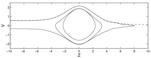
Figure 6.2: $(Z,V)$ phase space plots of captured and transmitted trajectories just above (dashed) and below (solid) critical velocity.

6.2 Experiment 2: medium $\eta$.

In Figure 6.3, computed for $\eta=2$, we see a quite different picture. Here and in the third numerical experiment, below, $-\eta^{2}/2<-\gamma^{2}/2=-1/2$ and resonant interactions can and do take place (cf. Figure 2.1). In this case there is no transition between transmission and reflection: the soliton travels monotonically rightward and is always transmitted without transient capture or oscillations about the defect. More strikingly, the output velocity appears to approach a finite limit $V_{\rm out}\approx 1.17$ as $V_{\rm in}\to 0$, while the amount of energy captured approaches $a-1\approx 1.26$ (all the soliton’s energy would be captured if $a-1=2$). As the initial velocity increases, so does the output velocity, while the energy transferred from the soliton to the defect mode decreases. This is not surprising, since the duration of the interaction decreases with increasing soliton speed.

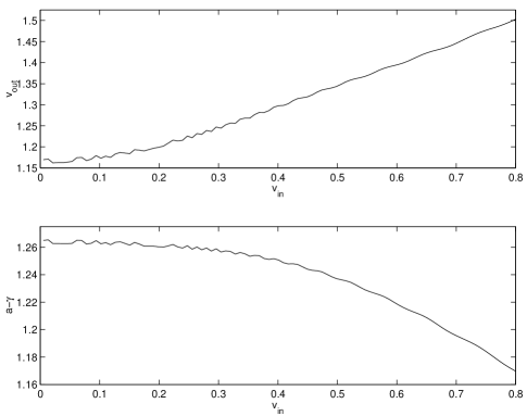
Figure 6.3: (Top) Outgoing velocity parameter V vs. incoming V of solitons incident on defect via ODE simulation with $\eta=2$. (Bottom) Amplitude $a-1$ of nonlinear defect mode after passing of the soliton.

6.3 Experiment 3: small $\eta$.

For Figure 6.4, we set $\eta=0.5<\gamma$; in this case the soliton is reflected if $V_{\rm in}$ lies below a critical velocity $V_{c}\approx 0.51$ and transmitted if $V_{\rm in}>V_{c}$. We also see that the defect mode has a final amplitude of order $10^{-3}$, absorbing little of the soliton’s energy. We note that $-\gamma^{2}/2=-1/2<-\eta^{2}/2$ corresponds to the region in Figure 2.1 in which the soliton has no resonant defect mode ‘partner’ with the same temporal frequency, and hence that appreciable interactions are unlikely [2].

Figure 6.5 shows evidence that the solution passes near $Z=V=0$, presumably approaching and leaving the neighborhood of a hyperbolic invariant set on this subspace. In Section 7 we shall show that this subspace indeed contains a fixed point of saddle-center type surrounded by a family of periodic orbits whose stable manifolds serve as separatrices. In Figure 6.5 we also show projections onto $(Z,V)$-space of the numerically determined stable and unstable manifolds of the fixed point, along with two trajectories: one with asymptotic velocity larger than the limiting value on the unstable manifold, which is transmitted, and one with asymptotic velocity smaller than the limiting velocity, which is reflected.

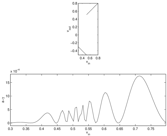
Figure 6.4: (Top) Outgoing velocity vs. incoming velocity of solitons incident on the defect via ODE simulation with $\eta=\frac{1}{2}$. (Bottom) Amplitude $a-1$ of nonlinear defect mode after passing of the soliton; note vertical scale is ${\mathcal{O}}(10^{-3})$.

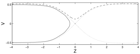
Figure 6.5: Phase space projections of trajectories above (solid) and below $V_{c}$ (dashed), showing strong evidence for a saddle point. Projections of stable and unstable manifolds of the saddle on ${{\mathcal{P}}_{0}}$ are shown as dotted curves.

7 Analysis of ordinary differential equations

The numerical experiments described above reveal two broad types of behavior. For small values of $\eta$, the soliton traveling near the critical velocity appears to approach a hyperbolic fixed point or periodic orbit on $(Z,V)=(0,0)$: see Figure 6.5. For larger values of $\eta$, it oscillates about $(Z,V)=(0,0)$ as if around an elliptic fixed point, and also follows orbits asymptotic to $(Z,V)=(\pm\infty,0)$ before turning: see Figure 6.2. To interpret these observations we now analyze the ODE system (5.9), seeking a (partial) understanding of its global phase space structure.

We first note that the sets $a=c$ and $a=1$ are invariant for the flow (although the vector field is singular on the latter), and bound the physically admissible region. When $a=1$ all the energy resides in the soliton; when $a=c$ it all resides in the defect mode. Letting ${{\mathcal{I}}}=[1,c]$ denote the closed interval, the phase space of Equation (5.9) is $(Z,V,\psi,a)\in\mathbb{R}^{2}\times S^{1}\times{{\mathcal{I}}}$. We also note the following (reversibility) symmetry group under which (5.9) is equivariant:

$$(Z,V,\psi,a,t) \rightarrow(-Z,V,2\pi-\psi,a,-t),$$ (7.1a)

$$(Z,V,\psi,a,t) \rightarrow(Z,-V,2\pi-\psi,a,-t).$$ (7.1b)

We shall use this below.

There is a family of solutions at $Z=\pm\infty$ with $V$, $a$, and $\dot{\psi}$ constant, which correspond to the uncoupled propagation and oscillation of the two modes when the soliton is infinitely far from the defect. The subset of these solutions with $V=0$ form a degenerate family of periodic orbits ‘at infinity,’ parameterized by $a=a_{\infty}$ and filling the annulus (or finite cylinder)

$${{\mathcal{P}}_{\infty}}=\{(\psi,a)|V=0,\;|Z|=\infty\}.$$ (7.2)

We note that by (5.9c) and (5.7), $\dot{\psi}=(\eta^{2}-a_{\infty}^{2})/2$ on ${{\mathcal{P}}_{\infty}}$, so that the frequency of these orbits is nonzero provided $a_{\infty}\neq\eta$ or, equivalently, $a_{\infty}\neq c/2$. As in [5] we may employ a transformation of the form $q=\operatorname{sech}Z,\;p=V$ to bring these orbits to the origin in $(p,q)$-space, and then apply McGehee’s stable manifold theorem [25] to prove the existence of invariant manifolds for the fixed point $(p,q)=(0,0)$ in an appropriate (local) Poincaré map. This shows that each periodic orbit in ${{\mathcal{P}}_{\infty}}$ has two-dimensional stable and unstable manifolds, so that $W^{s}({{\mathcal{P}}_{\infty}})$ – the stable manifold of ${{\mathcal{P}}_{\infty}}$ itself – is three dimensional and hence locally separates the four-dimensional phase space. Indeed, $W^{s}({{\mathcal{P}}_{\infty}})$ separates orbits that escape to infinity (transmitted solitons) from those that are reflected to interact with the defect mode again.

Studying the analogous sine-Gordon kink-trapping problem in [5], we used isoenergetic reduction and Melnikov’s method [26, 27] to prove that the stable and unstable manifolds of each periodic orbit, restricted to their common energy manifold, intersect transversely, and hence that Smale horseshoes exist [27]. We then appealed to phase space transport theory [28, 29] to unravel the structure of sets of initial data that are transiently captured before eventually being transmitted or reflected. We proceed in the same manner in Section 7.1, although we have to introduce an artificial small parameter, and the set of solutions to which the standard reduction procedure applies is limited, since it requires that the frequency $\dot{\psi}$ not change sign (in the process one replaces time by $\psi$), and this holds only for large $c$, depending on $a$; cf. Equation (5.9c). In particular, it does not hold for many physically relevant parameter values, including those corresponding to initial data with (almost) all the energy in the soliton $(a\approx 1)$. Nonetheless, the analysis does provide some understanding of the large $\eta$ simulations of Section 6.1.

There are further invariant manifolds that play an important rôle in the fate of solutions. They belong to orbits on a second annulus

$${{\mathcal{P}}_{0}}=\{(\psi,a)|V=0,\;Z=0\}$$ (7.3)

that is also invariant under the flow, and on which the ODEs are integrable. Solutions on ${{\mathcal{P}}_{0}}$ correspond to a soliton stalled over the defect and periodically exchanging energy with the defect mode. The orbit structure on ${{\mathcal{P}}_{0}}$ depends upon $c$ and may be derived from the level sets of the Hamiltonian function $H$ restricted to ${{\mathcal{P}}_{0}}$:

$$H_{{\mathcal{P}}_{0}}(\psi,a)=-\frac{c^{3}}{3}+(c-a)\left(ca-(c-a)-2\sqrt{a^{2}-1}\cos\psi\right).$$ (7.4)

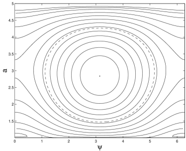
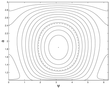
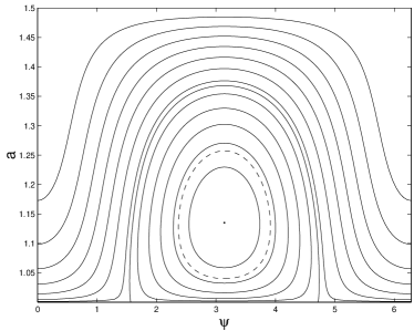
Figure 7.1: Level sets of $H_{0}$ in the invariant plane ${\mathcal{P}}_{0}$ for (a): $c=5\ (\eta=4)$; (b) $c=3\ (\eta=2)$ and (c) $c=1.5\ (\eta=0.5)$. The dashed curve indicates the boundary of the orbits accessible from infinity, as described in the text.

As noted above, the boundaries $a=c$ and $a=1$ of ${{\mathcal{P}}_{0}}$ are invariant, and the flow is singular on the latter, which contains two degenerate saddle points at $\psi=\pi/2,\;3\pi/2$. There is a unique fixed point $(\pi,a^{*})$ on $\psi=\pi$ surrounded by periodic orbits which limit on heteroclinic orbit(s). As shown in the first section of the Appendix, for all $c\;(>1)$, $(\pi,a^{*})$ is a saddle-center, with positive and negative real eigenvalues whose eigenvectors point out of ${{\mathcal{P}}_{0}}$. For $c<2.214\ldots$ this is the only equilibrium; for $c>2.214\ldots$ two further fixed points, a center-center and a saddle-center, appear on $\psi=0$; restricted to ${{\mathcal{P}}_{0}}$ these are a center and a saddle, whose separatrices interact with the stable and unstable manifolds of the degenerate saddles on $a=1$ in a heteroclinic bifurcation [27] at $c\approx 3.21$ as $c$ continues to increase. $H_{0}$ takes its minimum value $-c^{3}/3$ on $c=a$, its maximum at $(\pi,a^{*})$, and the value $-c^{3}/3+c-1$ on $a=1$ and the invariant manifolds emanating from it. Figure 7.1 shows these distinct cases. On this figure we also show the level set with Hamiltonian value equal to that of a ‘pure’ soliton stalled at infinity: $H(|Z|=\infty,V=0,a=1,\psi)=-c^{3}/3+c(c-1)$. Since any incoming soliton with nonzero speed has $H>-c^{3}/3+c(c-1)$ (see (5.8)), this curve bounds the set of accessible orbits on ${{\mathcal{P}}_{0}}$: a disk centered on $(\pi,a^{*})$.

7.1 Stable and unstable manifolds of ${{\mathcal{P}}_{\infty}}$

We first observe that we may define a local three-dimensional cross section [27] for the flow of (5.9):

$$\Sigma_{\pi}=\{(Z,V,\psi,a)|a\in(a^{*},c),\psi=\pi\}.$$ (7.5)

We verify that the flow is transverse to $\Sigma_{\pi}$ in the second section of the Appendix.

Since the Hamiltonian (5.8) is time-independent, its value is conserved by solutions of (5.9), which are therefore constrained to lie on three-dimensional surfaces

$$H(V,\psi,p,I;c)=h=\text{const},$$

determined by the initial data. The variables $p$ and $I$, defined below, denote coordinates which are conjugate to coordinates $V$ and $\psi$. As shown in the final section of the Appendix, this permits a further reduction in dimension. Specifically, since the cross section $\Sigma_{\pi}$ intersects level sets of $H$ transversely, $\Sigma_{\pi}$ may be used as a two-dimensional cross section for the flow restricted to constant $H$ surfaces. It is on this cross section that we will portray the stable and unstable manifolds $W^{s,u}({{\mathcal{P}}_{\infty}})$.

To approximate these manifolds we first add an artificial coupling parameter $\mu$ to the Hamiltonian of Equation (5.8):

$$H=-\frac{c^{3}}{3}+(c-a)\left(ca+V^{2}-(c-a)\operatorname{sech}^{2}Z\right)-\mu 2(c-a)\sqrt{a^{2}-1}\operatorname{sech}Z\cos\psi.$$ (7.6)

For the case at hand, $\mu=1$, but we shall assume $\mu\ll 1$ and perform a perturbative analysis, subsequently appealing to continuation to extend to $\mu=1$. The variables $V$ and $\psi$ are canonical ‘positions’ for this Hamiltonian with conjugate ‘momenta’ $p=-2Z$ and $I=2(a-\gamma)=2(a-1)$, and $I$ and $\psi$ are action-angle variables for the ‘second’ degree of freedom. In these canonical variables, the Hamiltonian (7.6) assumes the form:

$$H=H_{0}(V,p;I)+\mu H_{1}(p;I,\psi).$$ (7.7)

The formal discussion of the Melnikov integral will refer to these canonical variables, although in both the computations to follow, and in numerical simulations, it is more convenient to work with the original variables $(Z,V,\psi,a)$.

For $\mu=0$, the ‘unperturbed’ Hamiltonian $H_{0}$ is independent of $\psi$, and the ODEs reduce to

$$\dot{Z} =(c-a)V,$$ (7.8a)

$$\dot{V} =-(c-a)^{2}\operatorname{sech}^{2}{Z}\tanh{Z}$$ (7.8b)

$$\dot{\psi} =\frac{c^{2}-2ca-V^{2}}{2}+(c-a)\operatorname{sech}^{2}{Z}$$ (7.8c)

$$\dot{a} =0.$$ (7.8d)

The position and velocity $Z$ and $V$ evolve as a particle in a potential well, with the strength of the well dependent on $a=a_{0}$, which is unchanging. The solution set comprises bounded periodic orbits, and unbounded orbits where $\lvert Z\rvert\to\infty$ with finite speed. In between is a separatrix, on which $Z=\sinh^{-1}{\eta_{0}^{3/2}t}$, where $\eta_{0}=c-a_{0}$ is the amplitude of the soliton. In the unperturbed dynamics, the angular displacement, determined by integration of (7.8c) along the separatrix, is given by

$$\psi=\psi_{0}+\frac{\eta_{0}^{2}-a_{0}^{2}}{2}+\frac{1}{2\sqrt{\eta_{0}}}\arctan{\eta_{0}^{3/2}}.$$ (7.9)

The separatrices are homoclinic orbits to a periodic orbit $\beta(t)\in{{\mathcal{P}}_{\infty}}$ with $a=a_{0}$ and $(Z,V)=(\pm\infty,0)$. Note that unlike in [5] and related problems in celestial mechanics (e.g. [30]), in this case the generalized ‘position’ (soliton speed, $V$) goes to zero and the conjugate ‘momentum’ (soliton position, $Z$) goes to infinity.

We ask if any members of this continuum of homoclinic orbits persist when $\mu\neq 0$. Now if $W^{u}(\beta)$ crosses the $p=0$ axis at the point $(p=0,V,\psi=0,a,t=0)$, then, by the symmetries (7.1), $W^{s}(\beta)$ must also pass through this point. To establish existence of a (perturbed) homoclinic orbit it therefore suffices to show that either $W^{s}(\beta)$ or $W^{u}(\beta)$ intersects $p=0$. However, to demonstrate transverse intersections requires a more delicate calculation, appealing to perturbation theory for small $\mu$ and a result due to Melnikov, the derivation of which is outlined in the final section of the Appendix. Specifically, we have:

Theorem 2

Let $h>0$ and $\Omega_{0}(t)=\frac{\partial H_{0}}{\partial I}$. Let $\{H_{0},\frac{H_{1}}{\Omega_{0}}\}$denote the Poisson bracket of $H_{0}(V^{0},p^{0})$ and $H^{1}(V^{0},p^{0},\psi^{0},I^{0})/\Omega_{0}(V^{0},p^{0})$ evaluated along $V^{0}(t)$ and $p^{0}(t)$. Define the Melnikov function

$$M(\psi_{0})=\int_{-\infty}^{\infty}\left\{H_{0},\frac{H_{1}}{\Omega_{0}}\right\}(V,p^{0},\psi^{0},I^{0})(t)\ dt,$$ (7.10)

and assume that $M(\psi_{0})$ has a simple zero and $\Omega_{0}(t)\neq 0$. Then for $\mu>0$ sufficiently small, the Hamiltonian system has transverse homoclinic orbits on the energy surface $H=h^{0}$.

We note that the usual reduction process and Melnikov integral are meaningful only as long as $\psi$ is monotonic with respect to $t$ ($\dot{\psi}=\Omega\neq 0$), so that the global cross section $\Sigma_{\psi_{0}}$ referred to in the Appendix may be defined. However, Holmes [31] has extended this analysis to the case where $\dot{\psi}$ is allowed to change sign in a bounded region in the ‘middle’ of the unperturbed homoclinic orbit, but under the condition that $\psi$ be monotonic sufficiently close to the periodic orbit $\beta$. Direct substitution of the unperturbed orbit $Z=\sinh^{-1}{\eta_{0}^{3/2}t}$ into Equation (7.8c) yields

$$\Omega_{0}=\frac{1}{2}\left(\eta_{0}^{2}-a_{0}^{2}+\frac{\eta_{0}}{1+\eta_{0}^{3}t^{2}}\right).$$ (7.11)

By our ansatz $\eta_{0}>0$, and so the condition that $\Omega_{0}$ not change sign throughout is

$$(1<)\ a_{0}<\eta_{0}\text{ or }a_{0}>\sqrt{\eta_{0}^{2}+\eta_{0}};$$

however, if we appeal to [31], we need only exclude a neighborhood of the degenerate set

$$a_{0}=\eta_{0}$$

to ensure that $\Omega_{0}\neq 0$ near $\beta$.

We now sketch the computation needed to verify the remaining hypothesis of Theorem 2. Since $H_{1}$ is $V$-independent, the Poisson bracket reduces to

$$\left\{H_{0},\frac{H_{1}}{\Omega_{0}}\right\}_{(V,p)}=\frac{1}{\Omega_{0}}\frac{\partial H_{0}}{\partial V}\frac{\partial H_{1}}{\partial p}-\frac{H_{1}}{\Omega_{0}^{2}}\left(\frac{\partial H_{0}}{\partial V}\frac{\partial\Omega_{0}}{\partial p}-\frac{\partial H_{0}}{\partial p}\frac{\partial\Omega_{0}}{\partial V}\right).$$

After computing partial derivatives (cf. (7.8)) and substitution of the unperturbed separatrix solution in the Hamiltonian of (7.6), some manipulations, and appeal to odd- and evenness properties, the Melnikov integral may be written as:

$${\mathcal{M}}(\psi_{0})=\eta_{0}^{4}\sqrt{a_{0}^{2}-1}\left(\int_{-\infty}^{\infty}\frac{\left(-(\eta_{0}^{2}-a_{0}^{2})g(t)+\eta_{0}g^{-1}(t)\right)\sin{\Theta(t)}}{\left(\left(\eta_{0}^{2}-a_{0}^{2}\right)g^{2}(t)+\eta_{0}\right)^{2}}\,dt\right)\sin{\psi_{0}},$$ (7.12)

where

$$g(t)=\sqrt{1+\eta_{0}^{3}t^{2}}\text{ and }\Theta(t)=\frac{\eta_{0}^{2}-a_{0}^{2}}{2}t+\frac{1}{2\sqrt{\eta_{0}}}\arctan{\eta_{0}^{\frac{3}{2}}t}.$$

This integral cannot, in general, be computed explicitly, unless $\sqrt{\eta_{0}}$ is rational. However, since the integrand is an analytic function of $t$ with no essential singularities, it can have only isolated zeros. Therefore, except for special values of $(\eta_{0},a_{0})$, ${\mathcal{M}}(\psi_{0})$ has only simple zeros where $\psi_{0}=n\pi$, and Theorem 2 implies that, for small values of $\mu$, there exist transverse homoclinic orbits to infinity.

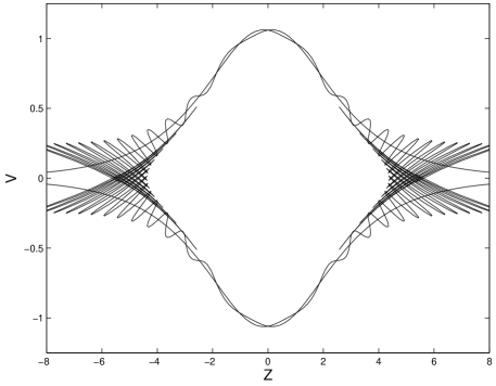
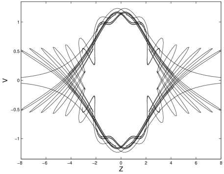
Figure 7.2: Stable and unstable manifolds of periodic orbits $\beta\in{\mathcal{P}}_{\infty}$, shown via the Poincaré map defined on the cross section $\Sigma_{\pi}$. (a) $\mu=0.25$; (b) $\mu=0.5$, corresponding to the energy level for $\eta=4$ and $V=0.4$.

Figure 7.2 shows numerical computations of the stable and unstable manifolds of periodic orbits in ${\mathcal{P}}_{\infty}$ for two values of $\mu$ in the same energy surface $H=-20.69$, corresponding to the energy of the system with a soliton with $\eta=4$ and $V=0.4$ starting at $\lvert Z\rvert=\infty$, with $a=0$. They are illustrated as curves lying in the cross section $\Sigma_{\pi}$ introduced at the beginning of this section. (Since each periodic orbit $\beta$ in ${\mathcal{P}}_{\infty}$ is a one-dimensional circle, $W^{s}(\beta)$ and $W^{u}(\beta)$ are each two-dimensional, and so intersect suitable cross sections to the flow in one-dimensional curves.) The transverse intersections are clear from the figure. As described in [5], phase space transport theory [28, 29] may be used to analyse the capture, transmission and reflection dynamics implied by transveral homoclinic points such as those of Figure 7.2. Here we provide a brief review; for a more complete explanation, see [5].

We consider $W^{u}(Z=-\infty)$, the unstable manifold of $Z=-\infty$, and $W^{s}(Z=\infty)$, the stable manifold of $Z=\infty$, which intersect transversely in a point $q_{0}$ in the top center of the figure. (Both cases show such an intersection, although the phenomenon is clearer in the lower figure.) The union of the point $q_{0}$, the portion of $W^{u}(Z=-\infty)$ to the left of $q_{0}$, and the portion of $W^{s}(Z=\infty)$ to the right of $q_{0}$ form a boundary between the upper and middle regions of the plane. A similar boundary exists in the lower half plane. Stretching off to the left from the point $q_{0}$ is a series of lobes lying in the upper region, each of which is the image under the map $P_{\pi}$ of the lobe to its left. Between each such pair of lobes in the upper region, and below $W^{u}(Z=-\infty)$, lies a lobe in the middle region. Counting both sets of lobes, the image of any given lobe under $P_{\pi}$ is the second lobe to its right. In particular, the image of the nearest upper region lobe to the left of $q_{0}$ is a lobe located in the middle region. Similarly, the image of the middle region lobe immediately to the left of $q_{0}$ lies in the upper region. This nearest upper lobe and the neighboring middle lobe form a turnstile through which phase space points are transported from the upper to the middle region, and from the middle to the upper region. A similar turnstile in the lower half plane transports phase space between the lower and middle regions.

Trapping takes place when an initial condition that lies in the sequence of lobes in the upper-left quadrant is mapped from the upper region to the middle region. Reflection or transmission occurs because eventually, as the interior lobes are successively stretched and folded, the image of this point will, with probability one, lie in a turnstile exit lobe (area preservation of the symplectic map $P_{\pi}$ guarantees that no open set contained in a preimage of an incoming turnstile lobe can be trapped for all future time [5, Proposition 1]). If the point’s image exits into the upper region, it is transmitted. If it goes into the lower region, it is reflected. This may be seen as an analogy with phase space transport in a two-bend horseshoe map, as is shown in [5]. The iterated preimages of the turnstile lobes forms a fractal structure that is responsible for the multiple reflection and transmission windows of Figure 6.1.

7.2 Stability of orbits on ${{\mathcal{P}}_{0}}$

To determine the stable and unstable manifolds of ${{\mathcal{P}}_{0}}$ we must first determine the stability types of orbits within it, to perturbations out of ${{\mathcal{P}}_{0}}$. By continuity, the periodic orbits immediately surrounding the saddle center $(\pi,a^{*})$ are also of saddle type with respect to such perturbations, but the stability types of other periodic orbits must be determined via Floquet theory [32].

On ${{\mathcal{P}}_{0}}$ the ODEs reduce to:

$$\dot{\psi} =\frac{c^{2}}{2}-ca+(c-a)+\frac{(2a^{2}-ac-1)}{\sqrt{a^{2}-1}}\cos{\psi},$$ (7.13a)

$$\dot{a} =-(c-a)\sqrt{a^{2}-1}\sin{\psi}.$$ (7.13b)

Typical phase portraits of (7.13) are shown in Figure 7.1 above.

Consider the solution ${\mathcal{S}}^{*}$ to the initial value problem of a soliton starting from $\lvert Z\rvert=\infty$ with finite velocity $V_{\infty}$ and zero energy in the defect mode, i.e. $a=1$ and $c=\eta+1$. ${\mathcal{S}}^{*}$ is confined to the level set

$$H=-\frac{c^{3}}{3}+(c-1)(c+V_{\infty}^{2})\stackrel{{\scriptstyle\rm{def}}}{{=}}H_{\infty}$$ (7.14)

of the conserved Hamiltonian and hence, if it approaches ${{\mathcal{P}}_{0}}$, can only interact with orbits having the same $H$-value. In particular, since the maximum $H$ value for orbits on ${{\mathcal{P}}_{0}}$ is assumed by the fixed point $(\pi,a^{*})$, there is a critical velocity $V_{\infty}^{\rm max}$ above which the solutions ${\mathcal{S}}^{*}$ have more ‘energy’ than any orbits contained in ${{\mathcal{P}}_{0}}$, and thus must remain bounded away from it. Similarly, the minimal value $H=-c^{3}/3+c(c-1)$ of orbits ${\mathcal{S}}^{*}$, assumed when $V_{\infty}=0$, bounds the set of accessible orbits on ${{\mathcal{P}}_{0}}$, as shown by the dashed curve on Figure 7.1.

Consequently, for each $V_{\infty}\in[0,V_{\infty}^{\rm max})$, we find a periodic orbit ${{\mathcal{S}}_{0}}\in{{\mathcal{P}}_{0}}$ with the same Hamiltonian value $H=h_{0}$ as ${\mathcal{S}}^{*}$ and determine its stability by examining the linearization of the full system (5.9) about ${{\mathcal{S}}_{0}}=(0,0,\psi_{\mathcal{P}}(t),a_{\mathcal{P}}(t))$. The stability of such an orbit is given by the eigenvalues of the monodromy matrix: the fundamental solution matrix of the linearized differential equation, evaluated at one period of oscillation. Let $\tilde{{\mathcal{S}}_{0}}=(\tilde{Z},\tilde{V},\tilde{\psi},\tilde{a})$ solve this linearized ODE, which is block-diagonal, with the $(\tilde{Z},\tilde{V})$ components decoupling from the $(\tilde{\psi},\tilde{a})$ components. The eigenspace of the latter coincides with ${{\mathcal{P}}_{0}}$ and hence they have eigenvalues of unit modulus, as one expects from the integrable structure of Figure 7.1 (in fact $\lambda=1$ with multiplicity two and a single eigenvector).

Perturbations perpendicular to ${{\mathcal{P}}_{0}}$ satisfy

$$\begin{split}\frac{d}{dt}{\tilde{Z}}&=(c-a_{\mathcal{P}}(t))\tilde{V},\\ \frac{d}{dt}{\tilde{V}}&=-\left((c-a_{\mathcal{P}}(t))^{2}+(c-a_{\mathcal{P}}(t))\sqrt{a_{\mathcal{P}}(t)^{2}-1}\cos{\psi_{\mathcal{P}}(t)}\right)\tilde{Z}.\end{split}$$ (7.15)

Since this may be written in the form

$$\frac{d}{dt}\binom{\tilde{Z}}{\tilde{V}}=\begin{pmatrix}0&A_{1,2}(t)\\ A_{2,1}(t)&0\end{pmatrix}\binom{\tilde{Z}}{\tilde{V}},$$

the Floquet theory for Hill’s equation is applicable [32]. The product of the Floquet eigenvalues must be one, and their sum is given by the Floquet discriminant. If this is greater than two in absolute value, the periodic orbit is hyperbolic, i.e. unstable; if less than two, the orbit is elliptic, i.e. neutrally stable, transverse to ${{\mathcal{P}}_{0}}$. We approximate these discriminants by first numerically integrating the orbit $(a_{\mathcal{P}}(t),\psi_{\mathcal{P}}(t))$ for one period, and then computing the fundamental solution matrix for the linearized system (7.15), using interpolated data for the coefficients.

Since each periodic orbit in ${{\mathcal{P}}_{0}}$ corresponds, via its Hamiltonian level, to a velocity $V_{\infty}$ at $|Z|=\infty$, we plot in Figure 7.3 the Floquet discriminants as functions of $V_{\infty}$ for the three examples of Section 6.3. In the first case ($\eta=4$) there are two regions each of stability and instability, and the velocity range shown in Figure 6.1 corresponds to periodic orbits of elliptic type, consistent with the intuition from Figure 6.2, that solutions oscillate about ${{\mathcal{P}}_{0}}$. The critical velocity dividing capture and transmission, identified in Figure 6.1 is indicated by an asterisk. The second case of $\eta=2$ encompasses a range of stability and one of instability, and in the third (and simplest) case, with $\eta=\frac{1}{2}$, all orbits are hyperbolic. It is notable that $V_{\infty}^{\rm max}=0.51$ in this case, approximately equal to the critical velocity for transmission and reflection seen in Figure 6.4 (but see the detailed analysis in Section 7.3, below).

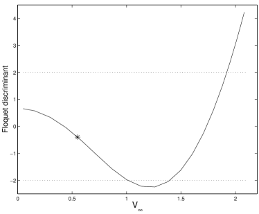
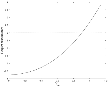
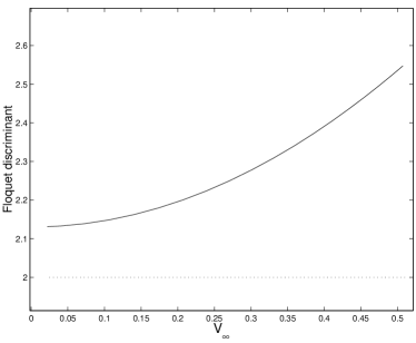
Figure 7.3: The Floquet discriminant vs. incoming velocity for $\eta={4},\,{2},\,\frac{1}{2}$ respectively (top to bottom). In the top panel, the critical velocity separating capture from transmission is marked with an asterisk.

Some interesting implications can immediately be drawn from the stability types of orbits in ${{\mathcal{P}}_{0}}$ implicit in Figure 7.3. Recall that these periodic orbits correspond to a state in which a soliton, stalled over the defect at $Z=0$, exchanges energy periodically with the defect mode. Hence, if soliton and defect parameters are chosen consistent with a stable region (eg., below $V_{\infty}\approx 0.9$ in case $\eta=2$ and for $V_{\infty}<1$ and $V_{\infty}\in(1.4,1.8)$ in case $\eta=4$), and the soliton is initialized at the defect or somehow introduced into it, perhaps by temporarily destabilizing the relevant orbit, it will remain trapped under small perturbations. Such stable trapped states do not exist for smaller $\eta$.

In the case $\eta=0.5$, the initial condition ${\mathcal{S}}^{*}_{c}=(-\infty,V_{c}=0.501,1,\psi_{0})$ lies on the same Hamiltonian surface as the fixed point $(\pi,a^{*})$. The stable and unstable manifolds of this fixed point are only one dimensional and thus cannot separate reflected from transmitted orbits. However, the stable and unstable manifolds of (the accessible disk on) ${{\mathcal{P}}_{0}}$ are three dimensional, and are consequently able to divide the phase space into disjoint regions. We must therefore compute the stable and unstable manifolds of the accessible periodic orbits on ${{\mathcal{P}}_{0}}$ as well as of the saddle-center $(\pi,a^{*})$.

7.3 Stable and unstable manifolds of ${{\mathcal{P}}_{0}}$

Appealing to the symmetries of (7.1) and the fact that the orbits of interest are reflection-symmetric about $\psi=\pi$, we need only compute one of the four branches of $W^{s,u}({{\mathcal{S}}_{0}})$ for each of the saddle type periodic orbits ${{\mathcal{S}}_{0}}\in{{\mathcal{P}}_{0}}$. To do this we first compute each periodic orbit ${\mathcal{S}}_{0}$ starting at a point $(a,\psi)=(a_{0},\pi)$ where $a_{0}>a^{*}$, the saddle-center. We interpolate these with 64 equally-spaced points (with respect to time). At each of these 64 points $(a_{0},\psi_{0})$, the fundamental solution matrix is computed as in Subsection 7.2. Fourier interpolation is used to compute the coefficients $(a_{\mathcal{P}},\psi_{\mathcal{P}})$ at intermediate times, so the orbit ${\mathcal{S}}_{0}$ need only be computed once. At each point on the periodic orbit, we compute the unstable eigenvector of the monodromy matrix, $\vec{v}_{0}=(Z_{0},V_{0})^{T}$. We normalize it so that $|\vec{v}_{0}|=10^{-5}$ and solve the full system (5.9) of ODE’s with initial conditions $(Z_{0},V_{0},a_{0},\psi_{0})$, stopping when $\lvert Z\rvert=20$.

Let $W^{s}({{\mathcal{P}}_{0}})=\cup_{h_{0}}W^{s}({{\mathcal{S}}_{0}})$ denote the set of stable manifolds of the accessible hyperbolic orbits in ${{\mathcal{P}}_{0}}$. $W^{s}({{\mathcal{P}}_{0}})$ is three dimensional, and is locally (near $|Z|=0$) foliated by two-dimensional cylinders, each of which is a local stable manifold of some ${{\mathcal{S}}_{0}}$. We therefore expect $W^{s}({{\mathcal{P}}_{0}})$ to intersect the three-dimensional cross sections of initial data $\Sigma_{\pm}=\{(V,\psi,a)|Z=\pm Z_{0},|Z_{0}|\gg 1\}$ in two-dimensional sets, which should in turn separate sets of initial data giving rise to solutions that pass the defect from those reflected by it.

Figure 7.4 shows the results of computations for the third of the three cases of Section 6: $\eta=0.5$, and for a further case, with slightly larger $\eta=0.75$. Note that the sets $\Sigma_{\pm}\sim\mathbb{R}\times S^{1}\times{{\mathcal{I}}}$ are periodic in $\psi$. As might be expected from the experiment of Section 6.3, near $a=1$ the surface $W^{s}({{\mathcal{S}}_{0}})\cap\Sigma_{-}$ is a graph over the $(\psi,a)$ annulus: all orbits starting at points below it are reflected, and points starting above it are transmitted. Further from $a=1$ the surface develops folds; these become more pronounced for higher $\eta\;(c)$, as in the lower panel of Figure 7.4. The surface describes the critical velocity as a function of phase $\psi$ and amplitude $a-1$ of the defect mode. Note the weak phase dependence, particularly as $a\rightarrow 1$, and that the surface approaches $a=1$ at $V\approx 0.51$ in the case $\eta=0.5$ (upper panel); this is the critical velocity found in Section 6.3. Initial data on this surface corresponds to trapping (recall that the accessible orbits in ${\mathcal{P}}_{0}$ correspond to solitons pinned at the defect).

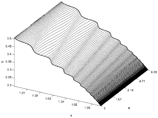
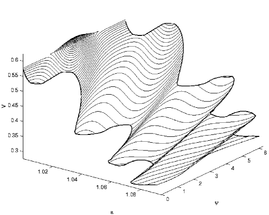
Figure 7.4: Part of the intersection of the stable manifold of ${{\mathcal{P}}_{0}}$ with $\Sigma_{-}$. (Top) $\eta=0.5\;(c=1.5)$; (bottom) $\eta=0.75\;(c=1.75)$.

In interpreting this figure it is helpful to note the following facts. Individual two-dimensional components $W^{s}({{\mathcal{S}}_{0}})$ of $W^{s}({{\mathcal{P}}_{0}})$ intersect sections at $Z=\pm Z_{0}$ for small $|Z_{0}|$ in homotopically trivial (contractible) circles, but as $|Z|$ (and the time of flight) increases, particular solutions belonging to $W^{s}({{\mathcal{S}}_{0}})$ can pass arbitrarily close to the degenerate saddles on $a=1$ at $\psi=\pi/2,3\pi/2$ (cf. Figure 7.1 (bottom)). This effectively separates neighboring solutions and stretches their phase ($\psi$) angles over a range exceeding $2\pi$. The result is that the corresponding sets $W^{s}({{\mathcal{S}}_{0}})\cap\Sigma_{-}$ extend around the $S^{1}$ component in a homotopically nontrivial manner. Only those components of $W^{s}({{\mathcal{P}}_{0}})$ very close to $W^{s}(\pi,a^{*})$ remain contractible; these can be seen in Figure 7.4 near $\psi=\pi,a=1$.

The ‘outer’ (lower $V$, higher $a$) boundary of the computed portion of $W^{s}({{\mathcal{S}}_{0}})\cap\Sigma_{-}$ is limited by numerical issues: it is impossible to compute with uniform accuracy as velocities approach zero, since the time of flight grows without bound; however, it appears that velocities do decrease to zero as $a$ increases. For example, numerical experiments like those of Section 6.3 indicate that all orbits launched with positive velocities, no matter how small, and $a>1.1$, are transmitted. The surface therefore intersects $V=0$.

We have been unable to reliably compute invariant manifolds of ${\mathcal{P}}_{0}$ for the medium and large $\eta$ cases. Preliminary studies suggest that, as $c$ increases, the set $W^{s}({{\mathcal{P}}_{0}})\cap\Sigma_{-}$ ‘separates’ from the plane $a=1$, so that nearby initial data all lie in the transmission zone (cf. Figure 6.3, which indicates that all solitons are transmitted for $\eta=2$, regardless of their initial velocities). However, as $c$ continues to increase, the stable manifold $W^{s}({{\mathcal{P}}_{\infty}})$ evidently invades $\Sigma_{-}$, leading to the complex behavior of Figure 6.1. In particular, the increased folding of $W^{s}({{\mathcal{P}}_{0}})\cap\Sigma_{-}$ as $\eta$ (or $c$) increases evident in Figure 7.4 is consistent with the existence of a fine (fractal) structure suggested by Figure 6.1. Since $W^{s}({{\mathcal{P}}_{\infty}})$ cannot intersect $W^{s}({{\mathcal{P}}_{0}})$, we conjecture that, as $W^{s}({{\mathcal{P}}_{\infty}})$ invades $\Sigma_{-}$, it must ‘align’ with the latter (folded) manifold, producing (infinitely) many regions of transmission and reflection on any vertical line in $\Sigma_{-}$ above the $(a,\psi)$-plane.

8 Interpretation and Summary

In this paper, we have derived a finite dimensional model for soliton-defect mode interactions in a nonlinear Schrödinger equation with a point defect. Following [1], and allowing for a fully nonlinear defect mode, which by itself is an exact solution, we derive a three-degree-of-freedom Hamiltonian system that describes the evolution of amplitudes and phases of the soliton and defect mode, and the position and velocity of the former. Allowing a nonlinear defect mode is important, since it permits resonant energy transfer to occur over a range of soliton amplitudes. However, only these two modes are represented; in particular, radiation to the continuum is ignored, and multiple solitons are disallowed.

The resulting ODEs may be further reduced to two degrees of freedom, since in addition to the Hamiltonian, a second quantity, corresponding to the total energy in the two modes, is also conserved. While this system is rather complex, and indeed is nonintegrable in certain parameter ranges (cf. Section 7.1), it possesses two-dimensional invariant subspaces filled with periodic orbits, whose stable and unstable manifolds partially determine the global structure of solutions. We use this system to investigate the reflection, transmission, and trapping of solitons launched ‘from infinity,’ by the defect, concentrating on the case in which the energy initially all resides in the soliton. Numerical simulations of the model ODE’s reveal three basic types of behavior:

1. For large initial soliton intensities, there is a critical velocity above which all solitons are transmitted; below this, a complex structure of reflection and transmission bands exists, separated by trapping regions that apparently are of measure zero. The capture and eventual transmission or reflection is explained by phase-space transport via turnstile lobes formed from parts of the stable and unstable manifolds of orbits ‘at infinity,’ corresponding to uncoupled oscillations of the defect mode and a distant soliton.

2. For moderate initial soliton intensities, all solitons are split into a transmitted part and a captured defect mode. The transmitted part travels to the right monotonically, giving up a fraction of its energy to the defect mode. The amount of energy transferred to the defect mode is a decreasing function of incident velocity.

3. For small initial soliton intensities, reflection or transmission occurs for almost all initial velocities. Specifically, a unique critical velocity exists for each initial phase and defect amplitude below a certain level; this represents initial data on the stable manifold of a subset of periodic orbits, each of which corresponds to the soliton stalled over the defect, periodically exchanging energy with the defect mode. This can be explained by the stable and unstable manifold of the manifold ${\mathcal{P}}_{0}$, which divide the phase space into two regions.

We now compare this to the behavior of the numerically computed solutions to the original PDE:

1. For large initial soliton intensities, there also exists a critical velocity separating solitons which are captured from those which pass by the defect with little interaction. The ODE prediction of $v_{c}=\eta V_{c}=2.21$ (with $\eta=4$) is in error by some $24\%$ compared to the PDE simulations, $v_{c}=1.78$, and unlike solutions to the ODE, captured PDE solitons do not eventually escape. The reduced ODE system is Hamiltonian, and thus, by a variant of the Poincaré recurrence theorem, any solution for which $Z$ is unbounded as $t\to-\infty$ must also have unbounded $Z$ at a later time, with probability 1. In the full PDE, however, radiation damping plays a role; there are radiative modes which carry energy away from the defect mode. These radiation modes are not incorporated in our Ansatz; as in other problems (cf. [5, 33]), their inclusion is expected to yield a collective coordinate ODE reduction with corrections which can play the role of damping. This damping corresponds to energy transfer from the soliton-defect mode subsystem to the radiative ‘heat bath.’ While the finite dimensional Hamiltonian ODE reduction leads to trapping for a set of data of measure zero, for the reduction perturbed by damping, a set of data of positive measure is trapped.

   The ODE model displays two behaviors for solitons below the critical velocity. Figure 6.1 reveals the existence of reflection windows: initial velocities for which the soliton returns to minus infinity with the same intensity and the opposite velocity it started with. Between these resonance windows are chaotic regions, where the soliton may oscillate near the defect any number of times before being ejected, with apparently random velocity. Reflection windows are a common feature of ODE models of this type [23, 21] as well as in some PDEs describing soliton–defect and soliton–soliton interactions [22, 24]. However, the fractal structure of the reflection/transmission windows is seen only in the ODE models and not in the PDEs. Radiation damping becomes important when the soliton stays in the neighborhood, and eliminates the chaotic behavior. It is shown in [5] that the chaotic behavior can be eliminated by the inclusion of appropriate radiation terms in the ODE ansatz, which leads to damping in the ODE.

   In numerical simulations of NLS soliton–defect interactions, no reflection windows have ever been found via PDE simulations. It appears from our simulations, and from a form of post-processing of the simulations to be described momentarily, that energy may be transferred from the soliton to the defect mode, but not vice-versa, so that once a defect mode is created, it never gives up its energy to the soliton. In the numerical post-processing, we calculate the six ODE parameters of (5.4) by minimizing the distance between the numerical PDE solution and the ODE ansatz defined by (5.2) and (5.3). In this analysis, for captured solutions $\eta$ decreases to zero as $a$ grows, so that the soliton is destroyed as the defect mode is created. This is in contrast with the sine-Gordon simulations of [23] in which reflection windows are seen. The difference lies in the fact that the two interacting modes in the sine-Gordon experiments are ‘topologically’ distinct. In that case the soliton is a kink, which approaches two different limits as $x\to\pm\infty$, while the defect mode is exponentially localized. The kink is defined solely by position and velocity, and has no amplitude parameter equivalent to $\eta$. When the kink transfers energy to the defect mode, it is not destroyed, since it still must satisfy the boundary conditions at $\pm\infty$. This topological constraint forces it to persist, so that energy stored in the defect mode may be (re-)converted to kinetic energy that pushes the kink away. In the NLS, in contrast, there is no such topological barrier, since the soliton decays to zero at both extremities. It can therefore transfer all its energy to the defect mode and cease to exist. No soliton-like structure need persist to absorb energy from the defect mode.

   This points to a criterion we have not seen mentioned when evaluating the effectiveness of collective coordinate ansatzen. If two modes included in an ansatz can become ‘far from orthogonal’ in some parameter regime, in that they may be highly correlated or may be used to represent the same information, then collective coordinate methods may give misleading results for solutions that approach these parameter regimes.

2. For intermediate intensities, and specifically $\eta=2$, the long time behavior consists of a captured defect mode and a transmitted soliton. The faster the soliton’s initial approach, the less energy is captured by the defect mode. Comparing Figure 4.4 with the lower graph of Figure 6.3, we see this ‘capture efficiency’ phenomenon in both cases. In neither case does a critical velocity separate captured from transmitted solitons.

3. For small intensities, the soliton is split into three parts: reflected, transmitted, and captured components. A prediction is made in [6] about the amount of energy in each of these three modes, although no comparison is made in numerics. Since the ansatz (5.2-5.3) permits only two modes, it cannot possibly capture all of this behavior. A three-mode ansatz, including two solitons and a defect mode, was constructed, but not found to be useful in studying this system. Nonetheless at very small (resp. large) initial velocities, the soliton is almost entirely reflected (resp. transmitted), so the two-mode ansatz is reasonable. In these cases, the initial condition lies squarely to one side or the other of the stable manifold illustrated in Figure 7.4, and the ODE and PDE simulations compare reasonably well. At intermediate velocities, the solution reaches a state shown in Figure 8.1, which is a reconstruction of the ansatz solution from the ODE parameters. In this figure, the solution appears as a soliton cleaved in two by a defect mode. In the full PDE, the two halves of the soliton component would separate and proceed in opposite directions. In the ODE reduction, they are unable to do that: the ansatz  (5.2-5.3) constrains recombination into a single soliton.

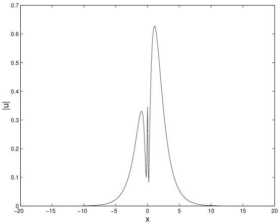
Figure 8.1: Reconstruction of the spatial structure of solutions from the two-mode ansatz (5.2-5.3), compared with full PDE solutions, for orbits reflected and transmitted in the case of $\eta=0.5$.

These comments illustrate what we believe to be rather general issues relevant to understanding the successes and failures of finite-dimensional or collective coordinate ODE reductions in reproducing PDE dynamics. Of course any correspondence between the solutions to a PDE and its variational ODE approximation depends on the assumption that the PDE solution remains close to the ansatz used in the approximation. This may or may not happen, and it is risky to draw quantitative information from the ODE model, for example regarding how solutions of the PDE depend on a certain parameter that is varied. Indeed, many such studies amount to numerically solving both the ODE and PDE, and noticing that the behavior is similar.

A more nuanced approach that is advocated in this paper and others, is that the ODE can be used to illuminate a mechanism that underlies a behavior seen in numerical simulations of the PDE. For example, we have seen that the existence of a critical velocity in the PDE can be explained by finding separatrices in the reduced ODE dynamics.

We may even take this a step further. An eventual goal of this research is to understand the behavior of gap solitons interacting with defects in Bragg gratings [2]. The derivation of a variational ODE for that system is complicated by the fact that gap solitons possess internal modes, which would require additional degrees of freedom in any collective coordinate ansatz, as in [34]. Nonetheless, NLCME gap solitons interacting with defects share many qualitative behaviors with the ODEs (5.9) derived in this study. We may draw a bifurcation diagram much like Figure 2.1 for this PDE. Further, low amplitude gap solitons are either coherently transmitted or reflected, whereas high amplitude gap solitons are captured when sufficiently slow, and pass by the defect if they have enough kinetic energy. Both of these behaviors were seen in the numerical experiments of Section 6. We may postulate that mechanisms similar to those seen in section 7 are responsible for the “resonance” between solitons and defects described in [2].

Acknowledgements:  RG was supported by NSF DMS-9901897 and Bell Laboratories/Lucent Technologies under the Postdoctoral Fellowship with Industry Program and by NSF DMS-0204881. PH was partially supported by DoE: DE-FG02-95ER25238. We thank D. Pelinovsky for stimulating discussions early in this project. Parts of this paper were presented at ‘Mathematics as a Guide to the Understanding of Applied Nonlinear Problems,’ a conference in honor of Klaus Kirchgässner’s 70th birthday, Kloster Irsee, Germany, Jan 6-10, 2002, and an early version appeared in the informal festschrift for that meeting, edited by H-J. Kielhöfer, A. Mielke, and J. Scheurle.

Appendix: Detailed calculations

Fixed points on ${{\mathcal{P}}_{0}}$

We verify the claim that the fixed points $(\psi,a)=(\pi,a^{*})$ on ${{\mathcal{P}}_{0}}$ are saddle centers. The center behavior within ${{\mathcal{P}}_{0}}$ follows from the structure of the restricted Hamiltonian (7.4), and behavior transverse to ${{\mathcal{P}}_{0}}$ is determined by the linearization given in (7.15), evaluated at $(\pi,a^{*})$. The resulting (constant) matrix has zero trace and determinant

$$D=(c-a^{*})^{2}\left((c-a^{*})-\sqrt{(a^{*})^{2}-1}\right)\stackrel{{\scriptstyle\rm{def}}}{{=}}(c-a^{*})^{2}\tilde{D}(a^{*}),$$ (8.1)

so, provided $\tilde{D}(a^{*})<0$, the remaining eigenvalues $\lambda=\pm\sqrt{-D}$ are real, implying hyperbolic saddle type behavior in the $(Z,V)$ directions. Note that $\tilde{D}(a^{*})<0$ iff

$$a^{*}>a_{c}=\frac{c^{2}+1}{2c}.$$ (8.2)

From (7.13) the fixed point value $a^{*}$ is given by solution of

$$L(a)\stackrel{{\scriptstyle\rm{def}}}{{=}}\frac{c^{2}}{2}+c-(c+1)a=\frac{(2a^{2}-ca-1)}{\sqrt{a^{2}-1}}\stackrel{{\scriptstyle\rm{def}}}{{=}}R(a).$$ (8.3)

Now $L(a)$ is monotonically decreasing and $R(a)$ is monotonically increasing (in the range $a\in(1,c)$), so if we can show that $L(a_{c})>R(a_{c})$, it follows that $a^{*}>a_{c}$ and hence that $\tilde{D}(a^{*})<0$, as required. But

$$L(a_{c})=\frac{(c^{2}-c-1)}{2c}\ \ {\rm{and}}\ \ R(a_{c})=-\frac{1}{c},$$

and so the claim is true.

The cross section $\Sigma_{\pi}$

To verify that $\Sigma_{\pi}=\{(Z,V,\psi,a)|a\in(a^{*},c),\psi=\pi\}$ is a cross section for the flow it suffices to show that $\dot{\psi}\neq 0$ on $\Sigma_{\pi}$. From (5.9c) we have

$$\dot{\psi}|_{\psi=\pi} = \frac{c^{2}-2ca}{2}-\frac{V^{2}}{2}+(c-a)\operatorname{sech}^{2}{Z}-\frac{(2a^{2}-ca-1)}{\sqrt{a^{2}-1}}\operatorname{sech}{Z}$$ (8.4)

$$= -\frac{V^{2}}{2}+(1-\operatorname{sech}Z)\left[\frac{c^{2}-2ca}{2}-(c-a)\operatorname{sech}Z\right]$$

$$\hskip 14.22636pt-\left(\frac{(2a^{2}-ca-1)}{\sqrt{a^{2}-1}}-\left[\frac{c^{2}-2ca}{2}+(c-a)\right]\right)\operatorname{sech}Z$$

$$\leq (1-\operatorname{sech}Z)\left[\frac{c^{2}-2ca}{2}-(c-a)\operatorname{sech}^{2}{Z}\right]$$

$$\hskip 14.22636pt-[R(a)-L(a)]\operatorname{sech}Z,$$

where $R(a)$ and $L(a)$ are defined in (8.3). Now $\operatorname{sech}Z<1$ for $|Z|<\infty$, so the sign of the leading term in (8.4) is determined by the expression in square brackets. The second term of this is always negative for $1<a<c$ and the first is also negative for $a>a^{*}$, since $a^{2}>a_{c}>c/2$, as shown above. Finally, since $R(a)$ is monotonically increasing and $L(a)$ monotonically decreasing and $a>a^{*}$, the point at which $R(a^{*})=L(a^{*})$, the last term is also strictly negative. We conclude that $\dot{\psi}<0$ on $\Sigma_{\pi}$, as required.

Reduction and the Melnikov function

We summmarise the modified reduction procedure and Melnikov calculation developed by Holmes and Marsden [35] for two degree-of-freedom Hamiltonian systems in the form (7.7), in which the frequency of the action-angle mode depends upon the phase variables in the other degree of freedom. (The procedure is also outlined in [36], where it is applied to Kirchhoff’s equations for equilibria of an elastic rod.) As in Melnikov’s ‘standard’ method [26, 27], transverse intersections of stable and unstable manifolds of a perturbed system are found by examining the zeros of an integral computed along the homoclinic orbit of the unperturbed system.

Consider the perturbed two-degree-of-freedom system with Hamiltonian

$$H=H_{0}(V,p;I)+\mu H_{1}(V,p;I,\psi)=h\;(=\rm{const.}),$$ (8.5)

and let

$$\Omega=\frac{\partial H_{\mu}}{\partial I}=\frac{\partial H_{0}}{\partial I}+O(\mu)=\Omega_{0}+O(\mu).$$ (8.6)

Then, provided $\Omega>0$, Equation (8.5) may be inverted and solved for $I$ in terms of $V$, $p$, $\psi$ and the constant $h$. As shown in [35], we may therefore eliminate $I$ and replace time by the conjugate variable $\psi$ and write the reduced three-dimensional system on the constant energy surface as a periodically forced single degree of freedom system with Hamiltonian $-I(V,p,\psi;L,h)$, and evolution equations

$$V^{\prime}=-\frac{\partial I}{\partial p},\quad p^{\prime}=\frac{\partial I}{\partial V},$$ (8.7)

where $(\cdot)^{\prime}$ denotes $d/d\psi(\cdot)$. This implies conservation of three-dimensional phase-space volume on the constant energy manifolds, and area preservation in the two-dimensional Poincaré maps defined below. Moreover, in [35] it is shown that the reduced Hamiltonian $I$ of (8.7) may be written

$$I={\mathcal{I}}_{0}(V,p;L,h)+\mu{\mathcal{I}}_{1}(V,p,\psi;L,h)+O(\mu^{2}),$$ (8.8)

where ${\mathcal{I}}_{1}$ is $2\pi$-periodic in $\psi$. Thus, reduction yields the standard form of a periodically perturbed single-degree-of freedom system for application of Melnikov’s method [26, 27]. In fact, inserting the series (8.8) into the Hamiltonian (7.7), we find

$${\mathcal{I}}_{0} =H_{0}(V,p)^{-1}(h),$$ (8.9)

$${\mathcal{I}}_{1} =-\frac{H_{1}(V,p,{\mathcal{I}}_{0},\psi)}{\Omega_{0}(V,p,{\mathcal{I}}_{0})}.$$ (8.10)

When $\mu=0$, the reduced Hamiltonian system (8.7) has a phase portrait which coincides with that of the full system, since the vector field is given by

$$\left(-\frac{\partial I}{\partial p},\frac{\partial I}{\partial V}\right)=\frac{1}{\Omega_{0}}\left(\frac{\partial H}{\partial p},-\frac{\partial H}{\partial V}\right);$$

it therefore also has a homoclinic orbit. When $\mu>0$, the system (8.7) is non-autonomous, and thus we may no longer draw a phase portrait, but we may instead construct the Poincaré map on the cross section $\Sigma_{\psi_{0}}=\{(V,p,\psi=\psi_{0})\}$ [27]. By a theorem of McGehee [25] the periodic orbit at infinity, $\beta$, and its stable and unstable manifolds $W^{s}(\beta)$ and $W^{u}(\beta)$ persist for small values of $\mu$.

To prove transverse intersection of $W^{s}(\beta)$ and $W^{u}(\beta)$, we apply the Melnikov method to the Poincaré map $P_{\psi_{0}}:\Sigma_{\psi_{0}}\to\Sigma_{\psi_{0}}$ that results from following the flow from $\psi=\psi_{0}$ to $\psi=\psi_{0}+2\pi$. As noted at the beginning of Section 7, and treated in greater detail for the analogous Sine-Gordon problem in [5], a result of McGehee [25] allows us to apply the Melnikov method even though the fixed point at infinity is not hyperbolic. The Melnikov integral can be interpreted as a normalized distance between the stable and unstable manifolds at a specified point on the cross section $\Sigma$. As in [36], we may then apply a version of the usual Melnikov method [26, 27] to the reduced system (8.7). This would lead to a Poisson bracket involving involving ${\mathcal{I}}_{0}$ and ${\mathcal{I}}_{1}$ in the Melnikov integrand, but, via Equations (8.9-8.10), this is equivalent to the ‘$p-V$’ Poisson bracket of the original functions $H_{0}$ and $H_{1}$. This yields Theorem 2 as stated in Section 7.1.

References

- [1] K. Forinash, M. Peyrard, B. Malomed, Interaction of discrete breathers with impurity modes, Phys. Rev. E 49 (1994) 3400–3411.
- [2] R. H. Goodman, R. E. Slusher, M. I. Weinstein, Stopping light on a defect, J. Opt. Soc. Am. B 19 (2002) 1635–1632.
- [3] Y. Kivshar, S. Gredeskul, A. Sánchez, L. Vázquez, Localization decay induced by strong nonlinearity in disordered systems, Phys. Rev. Lett. 64 (15) (1990) 1693–1696.
- [4] J. Bronski, Nonlinear scattering and analyticity properties of solitons, Journal of Nonlinear Science 8 (2) (1998) 161–182.
- [5] R. H. Goodman, P. J. Holmes, M. I. Weinstein, Interaction of sine-Gordon kinks with defects: Phase space transport in a two-mode model, Physica D 161 (2002) 21–44.
- [6] X. D. Cao, B. A. Malomed, Soliton-defect collisions in the nonlinear Schrödinger equation, Phys. Lett. A 206 (1995) 177–182.
- [7] S. Albeverio, F. Gesztesy, R. Hëgh-Krohn, H. Holden, Solvable models in quantum mechanics, Springer Verlag, New York, 1988.
- [8] R. Weder, The continuity of the Schrödinger wave operators on the line, Comm. Math. Phys. 208 (1999) 507–520.
- [9] T. Kato, G. Ponce, Commutator estimates and the Euler and Navier-Stokes equations, Comm. Pure Appl. Math. 41 (1988) 891–907.
- [10] V. E. Zakharov, A. B. Shabat, Exact theory of two-dimensional self-focusing and one dimensional self-modulation of waves in nonlinear media, Sov. Phys. JETP 34 (1972) 62–69.
- [11] H. A. Rose, M. I. Weinstein, On the bound states of the nonlinear Schrödinger equation with a linear potential, Physica D 30 (1988) 207–218.
- [12] M. I. Weinstein, Lyapunov stability of ground states of nonlinear dispersive evolution equations, Commun. Pure Appl. Math. 39 (1986) 51–68.
- [13] A. Soffer, M. I. Weinstein, Multichannel nonlinear scattering theory for nonintegrable equations, Commun. Math. Phys. 133 (1990) 119–146.
- [14] A. Soffer, M. I. Weinstein, Multichannel nonlinear scattering for nonintegrable equations II. the case of anistropic potentials and data, J. Diff. Eqns. 98 (1992) 376–390.
- [15] C.-A. Pillet, C. E. Wayne, Invariant manifolds for a class of dispersive, Hamiltonian, partial differential equations, J. Diff. Eqns. 141 (1997) 310–326.
- [16] V. S. Buslaev, G. Perel’man, Scattering for the nonlinear schrödinger equation: states close to a soliton, St. Petersburg Math. J. 4 (1993) 1111–1142.
- [17] R. Weder, Center manifold for nonintegrable nonlinear Schrödinger equations on the line, Comm. Math. Phys. 215 (2000) 343–356.
- [18] Z. Fei, V. M. Pérez-García, L. Vázquez, Numerical simulations of nonlinear Schrödinger systems: a new conservative scheme, Applied Math and Computation 71 (1995) 165–177.
- [19] B. A. Malomed, Variational methods in nonlinear fiber optics and related fields, Progress in Optics 43 (2002) 71–193.
- [20] V. Arnold, Mathematical Methods of Classical Mechanics, Springer Verlag, New York, 1978.
- [21] P. Anninos, S. Oliveira, R. Matzner, Fractal structure in the scalar model, Phys. Rev. D 44 (1991) 1147–1160.
- [22] D. Campbell, J. Schonfeld, C. Wingate, Resonance structure in kink-antikink interactions in theory, Physica D 9 (1983) 1–32.
- [23] Z. Fei, Y. S. Kivshar, L. Vázquez, Resonant kink-impurity interactions in the sine-Gordon model, Phys. Rev. A 45 (1992) 6019–6030.
- [24] J. Yang, Y. Tan, Fractal dependence of vector-soliton collisions in birefringent fibers, Phys. Lett. A 280 (2001) 129–138.
- [25] R. McGehee, A stable manifold theorem for degenerate fixed points with applications to celestial mechanics, J. Differential Equations 14 (1973) 70–88.
- [26] V. K. Melnikov, On the stability of the center for time periodic perturbations, Trans. Moscow Math. Soc. 12 (1963) 1–57.
- [27] J. Guckenheimer, P. Holmes, Nonlinear Oscillations, Dynamical Systems, and Bifurcations of Vector Fields, Springer-Verlag, New York, 1983.
- [28] V. Rom-Kedar, S. Wiggins, Transport in two-dimensional maps, Arch. Rational Mech. and Analysis 109 (1990) 239–298.
- [29] S. Wiggins, Chaotic Transport in Dynamical Systems, Springer-Verlag, New York, 1992.
- [30] H. Dankowicz, P. Holmes, The existence of transverse homoclinic points in the Sitnikov problem, J. Differential Equations 116 (1995) 468–483.
- [31] P. Holmes, Chaotic motions in a weakly nonlinear model for surface waves, J. Fluid Mech. 162 (1986) 365–388.
- [32] P. Hartman, Ordinary Differential Equations, second, corrected Edition, Wiley Publishing Co., New York., 1964.
- [33] A. Soffer, M. I. Weinstein, Resonances and radiation damping in Hamiltonian nonlinear wave equations, Invent. Math. 136 (1999) 9–74.
- [34] Z. Fei, Y. S. Kivshar, L. Vázquez, Resonant kink-impurity interactions in the model, Phys. Rev. A 46 (1992) 5214–5220.
- [35] P. J. Holmes, J. E. Marsden, Horseshoes and Arnol′d diffusion for Hamiltonian systems on Lie groups, Indiana Univ. Math. J. 32 (1983) 273–309.
- [36] A. Mielke, P. Holmes, Spatially complex equilibria of buckled rods, Arch. Rational Mech. Anal. 101 (1988) 319–348.