Instabilities and Spatio-temporal Chaos of Long-wave Hexagon Patterns in Rotating Marangoni Convection

Abstract

We consider surface-tension driven convection in a rotating fluid layer. For nearly insulating boundary conditions we derive a long-wave equation for the convection planform. Using a Galerkin method and direct numerical simulations we study the stability of the steady hexagonal patterns with respect to general side-band instabilities. In the presence of rotation steady and oscillatory instabilities are identified. One of them leads to stable, homogeneously oscillating hexagons. For sufficiently large rotation rates the stability balloon closes, rendering all steady hexagons unstable and leading to spatio-temporal chaos.

In the study of the formation of patterns the origin of spatial and temporal disorder is an important question. In recent years quite some progress has been made in the understanding of various states of spatio-temporal chaos that arise from stripe-like patterns, as they are found in the convection of fluids heated from below, or from spatially homogeneous oscillations. Much less is known about spatio-temporally chaotic states that are based on hexagonal patterns. We therefore investigate the classic surface-tension-driven Marangoni convection in a modification in which the system is rotated around a vertical axis. In buoyancy-driven roll convection such a rotation is known to induce chaotic dynamics through the Küppers-Lortz instability. In order to obtain a systematic reduced description of the fluid system we consider the case of long-wave convection and derive the appropriate order-parameter equation. Its stability analysis reveals regimes in which hexagons of all wavenumbers are unstable leading to a spatio-temporally chaotic state. In addition, homogeneously oscillating hexagon states are found.

1 Introduction

In the classic, buoyancy-driven Rayleigh-Bénard convection rotation of the system has been found to lead to very interesting new dynamic patterns. The origin of the dynamics is the Küppers-Lortz instability [1], which renders all straight roll patterns unstable with respect to a set of rolls rotated with respect to the original ones. It occurs above a critical rotation rate. In simple low-dimensional models the instability is found to a heteroclinic cycle connecting roll patterns rotated with respect to each other by $120^{o}$ [2, 3]. In experiments (e.g. [4, 5]) as well as in numerical computations of the Navier-Stokes equations (e.g. [5]) and of model equations (e.g. [6]) more complex behavior is found. Patches of convection rolls of various orientations arise and the roll orientation changes through the propagation of the fronts separating them or by the nucleation of rolls with a new orientation.

The other classic convection system is surface-tension-driven Marangoni convection of a liquid layer in contact with another liquid or a gas layer (for a recent review see [7]). Two different instability mechanisms have been identified that drive this type of convection: a short-wave instability, which occurs independent of any deflections of the interface [8] and a long-wave instability, for which deformations of the interface are essential [9, 10]. Not too far from threshold, the short-wave instability typically leads to convection patterns with hexagonal planform (e.g. [11, 12]), while the long-wave instability induces isolated dry spots or high spots [13, 14]. The stability of the hexagonal short-wave pattern with respect to sideband instabilities (the ’stability balloon’) has been determined in weakly nonlinear [15] and in fully nonlinear numerical approaches [16]. Further above onset the short-wave hexagon pattern is often observed to undergo a transition to squares [17, 18, 19, 11, 20, 12]. If the mean surface tension of the fluid is not too large the short-wave convection mode has to be coupled to a weakly damped long-wave mode that corresponds to the local layer height of the fluid [21, 22]. A different type of long-wave instability has been identified theoretically for the case when the fluid layer is bounded above and below by poor thermal conductors [8]. The mechanism for this instability is the same as for the short-wave instability. Due to the poor conductivity the critical wavenumber is, however, shifted to small values. Again one finds that near onset the planform is usually hexagonal. It turns out that experimentally this limit of long wavelengths is difficult to achieve. Theoretically, however, it is a very useful limit since it allows to derive simplified evolution equations systematically from the basic fluid equations without the restriction to small amplitudes, although restrictions on the control parameter remain [23, 24, 25]. Moreover, compared to the weakly nonlinear Ginzburg-Landau equations the long-wave equations have the additional great advantage of preserving the isotropy of the system. This will play an important role in the present paper.

With the interesting behavior ensuing from the Küppers-Lortz instability, it is natural to ask whether rotation has also an interesting impact on hexagonal convection patterns. Within the general context of small-amplitude expansions and Ginzburg-Landau equations this question has been addressed previously [26, 27, 28, 29, 30, 31, 32, 33]. These analyses were aimed at a general investigation of hexagonal patterns in rotating systems and apply also to weakly non-Boussinesq Rayleigh-Bénard convection. It was found that in a rotating system a new state of oscillating hexagons can appear. This transition replaces then the transition from hexagons to rolls that is obtained in non-Boussinesq Rayleigh-Bénard convection. In Marangoni convection this transition does not occur and no oscillating hexagons of this type are expected. Instead, in the absence of rotation a transition to squares is found [17, 18, 19]. The effect of rotation on this transition has not been studied yet. For the usual, steady hexagons the weakly nonlinear analysis indicates the possibility of persistent chaotic dynamics coexisting with the steady hexagons for the same parameter values [31]. However, these dynamics cannot be captured by the Ginzburg-Landau equations employed. To make reliable statements about this chaotic state, which is characterized by a spatially isotropic Fourier spectrum, equations have to be studied that preserve the isotropy of the system. A first step in this direction was the study of a Swift-Hohenberg model, which was generalized to capture the breaking of the chiral symmetry that characterizes the rotation. A detailed analysis of the resulting equation, which was not derived from any physical system, revealed that steady hexagons of all wavenumbers can become unstable already for amplitudes below the transition to the oscillating hexagons, leaving a range in the control parameter over which no simple periodic solution is stable [34] and in which chaotic dynamics are found in numerical simulations.

Motivated by the previous results of weakly nonlinear approaches to hexagons in rotating systems, our goal for the present paper is to obtain a systematic description of Marangoni convection in a rotating system that is not limited to small amplitudes and that preserves the isotropy of the system. We therefore turn to the long-wave limit that is obtained for poorly conducting top and bottom boundaries and extend the derivation of [23, 24] to the case of a rotating system. The poor heat conductivity is expressed in terms of a small Biot number $Bi$. While the true limit of long wavelengths ($Bi\ll 1$) may not be attainable in experiments [14] we expect to gain valuable insight into the system for moderate wavelengths by expanding in $Bi$. The form of the resulting long-wave equation is the same as that found for buoyancy-driven convection with poorly conducting boundaries [35] and for buoyancy-driven convection in binary mixtures with positive separation ratio [36]. In the latter case the critical wavenumber goes to 0 at a critical value of the separation ratio. In both cases quadratic terms arise only if the vertical symmetry is broken by imposing different boundary conditions at the top and the bottom plate (free-slip vs. no-slip or fixed temperature vs. fixed heat flux). The focus of [35] is the effect of rotation on the system. In contrast to our work, however, there the competition between strictly periodic roll and square planforms is considered. The work is performed analytically in the weakly nonlinear regime, supplemented by a few simulations of a small system.

In sec.2 we introduce the basic fluid equations and associated boundary conditions. The general linear stability analysis that identifies the long-wave regime is performed in sec.3. The long-wave equation is derived in sec.4. The stability and dynamics of the hexagon patterns is then studied numerically in sec.5. The main results of the simulations are periodic and chaotic dynamics arising from secondary instabilities of the hexagons as well as from a resonant mode interaction.

2 Formulation of the problem

2.1 Basic equations

We consider a thin viscous and incompressible fluid layer heated from below with a free surface and rotating around a vertical axis. The mean surface tension is assumed to be large enough to suppress surface deformations even in the presence of rotation. The Navier-Stokes and the heat equation then read

$${\rho}\left(\partial_{t}+{\bf v}\cdot\nabla\right){\bf v} = -\nabla p+\frac{\rho}{2}\nabla|\Omega{\bf e}_{z}\times{\bf r}|^{2}+2\rho\Omega{\bf e}_{z}\times{\bf v}+\eta\Delta{\bf v}-\rho g{\bf e}_{z},$$ (1)

$$\nabla\cdot{\bf v} = 0,$$ (2)

$$\left(\partial_{t}+{\bf v}\cdot\nabla\right)T = \kappa\nabla^{2}T.$$ (3)

In this paper we focus on fluid layers that are sufficiently thin that buoyancy can be ignored. The density is then taken to be constant, $\rho=\rho_{0}$. The dynamic viscosity $\eta$ is related to the kinematic viscosity $\nu$ through $via$ $\nu=\eta/\rho_{0}$ and $\kappa$ is the thermal diffusivity. The equations in dimensionless form can be obtained if the space, time, angular velocity, temperature, pressure and velocity fields are respectively divided by the constants $d$, $d^{2}/\kappa$, $\kappa/d^{2}$, $\Delta T$, $\rho_{0}\kappa\nu/d^{2}$ and $\kappa/d$. Here $d$ is the thickness of the fluid layer and $\Delta T$ is the temperature difference across the liquid layer in the conductive state. They are written as follows,

$$\frac{1}{\mathcal{P}}\left(\partial_{t}+{\bf u}\cdot\nabla\right){\bf u} = -\nabla p+\frac{\mathcal{P}}{2}\nabla|{\bf\Omega}\times{\bf r}|^{2}+2{\bf\Omega}\times{\bf u}+\nabla^{2}{\bf u}-{\mathcal{G}}{\bf e}_{z},$$ (4)

$$\nabla\cdot{\bf u} = 0,$$ (5)

$$\left(\partial_{t}+{\bf u}\cdot\nabla\right)\theta = \nabla^{2}\theta,$$ (6)

where ${\mathcal{P}}=\nu/\kappa$ is the Prandtl number and ${\mathcal{G}}=d^{3}\rho g/(\eta\nu)$ is the Galileo number. In this paper we consider the limit of infinite Prandtl number.

We eliminate the pressure from the Navier-Stokes equations (4) by using the incompressibility condition (2). Taking the curl and the double curl of (1) we obtain [37]

$$\nabla^{4}w-2\Omega\,\partial_{z}\zeta = 0,$$ (7)

$$\nabla^{2}\zeta+2\Omega\,\partial_{z}w = 0,$$ (8)

where $w$ is the $z$-component of the velocity ${\bf u}=(u,v,w)$ and $\zeta$ is the $z$-component of the vorticity $\nabla\times{\bf u}$. We also introduce the horizontal Laplacian $\Delta_{H}=(\partial^{2}_{xx}+\partial^{2}_{yy})$. Note that the rotation couples the vertical velocity and the vertical vorticity. Thus, while in the absence of rotation the vertical vorticity vanishes in many solutions of interest, with rotation the vertical vorticity is in general non-zero.

The equations for the $x$ and $y$-components of the velocity field are obtained considering that the velocity field ${\bf u}=(u,v,w)$ is expressed in terms of the poloidal and the toroidal stream functions $\phi$ and $\xi$ as follows: ${\bf u}=(\partial_{x}\partial_{z}\phi+\partial_{y}\xi,\partial_{y}\partial_{z}\phi-\partial_{x}\xi,-\Delta_{H}\phi)$. Then the equations for $u$ and $v$ are:

$$-\Delta_{H}u = \partial_{x}\partial_{z}w+\partial_{y}\zeta,$$ (9)

$$-\Delta_{H}v = \partial_{y}\partial_{z}w-\partial_{x}\zeta.$$ (10)

These equations together with (7)-(8) are equivalent to (4)-(5) [24].

2.2 Boundary conditions

In order to obtain the velocity boundary condition at the top free surface we take into account thermocapillary effects and assume a linear dependence of the surface tension on the temperature, $\sigma=\sigma_{0}-\gamma(T-T_{0})$. Furthermore, for sufficiently large mean surface tension and not too high rotation rates we can take the free surface to be flat. The boundary conditions at the upper free surface are then given by

$$\rho\nu\left(\frac{\partial w}{\partial x}+\frac{\partial u}{\partial z}\right) = -\gamma\left(\frac{\partial T}{\partial x}\right),$$ (11)

$$\rho\nu\left(\frac{\partial w}{\partial y}+\frac{\partial v}{\partial z}\right) = -\gamma\left(\frac{\partial T}{\partial y}\right).$$ (12)

After taking derivatives of (11) and (12) with respect to $x$ and $y$, respectively, and addition of both expressions, one is led to

$$\rho\nu\left(\frac{\partial^{2}w}{\partial z^{2}}\right) = -\gamma\Delta_{H}T.$$ (13)

Introducing the Marangoni number $M=\gamma d\Delta T/(\rho\nu\kappa)$ the boundary condition can be written as

$$\frac{\partial^{2}w}{\partial z^{2}} = M\Delta_{H}\theta\qquad\mbox{ at }z=1.$$ (14)

From the Marangoni equations (11-12) and from the underformability of the surface the other boundary conditions at the top are

$$w=\partial_{z}\zeta=0, {\rm at}\,z=1.$$ (15)

At the bottom we take no-slip boundary conditions for the velocity [38, 39, 40, 35],

$$w=\zeta=\partial_{z}w=0, {\rm at}\,z=0.$$ (16)

The critical wavenumber at which convection sets in depends sensitively on the temperature boundary conditions. Long wavelengths are obtained if the boundaries are poor conductors. The Newton law at the bottom plate can be expressed as

$${\rm k}\partial_{z}T_{fb} = h_{1}(T_{fb}-T_{b})\qquad\mbox{ at }z=0,$$ (17)

where $T_{fb}$ is the temperature of the fluid at the bottom plate and $T_{b}$ is the temperature of the plate at some distance below this interface. The thermal conductivity of the liquid is given by k and $h_{1}$ is the heat exchange coefficient at the bottom. We non-dimensionalize the temperature field by setting $\theta=(T-T_{fbc})/\Delta T$, where $T_{fbc}$ is the temperature of the fluid in the conductive state at the bottom plate and $\Delta T$ is again the temperature difference across the layer in the conductive state, i.e. $\Delta T=T_{fbc}-T_{ftc}$ with $T_{ftc}$ the upper temperature of the fluid in the conductive state. In terms of $\theta$ the boundary condition (17) is then given by

$$\partial_{z}\theta = Bi_{1}\theta-1\qquad\mbox{ at }z=0$$ (18)

with the Biot number $Bi_{1}=h_{1}d/{\rm k}$. Here we have made use of the conservation of heat flux at the interface, $h_{1}(T_{fbc}-T_{b})=-{\rm k}/d(T_{fbc}-T_{ftc})$. In a similar way the temperature boundary condition at the top is found to be

$$\partial_{z}\theta = -Bi_{2}\theta-1-Bi_{2}\qquad\mbox{ at }z=1.$$ (19)

These expressions agree with those used in [41] when the limit of a single layer is taken (in their notation this limit corresponds to $\Theta_{1}=\Theta_{2}$, $\kappa=1$ and $a=0$).

3 Linear stability analysis

In order to motivate the long-wavelength analysis we first discuss the linear stability of the conductive solution. The normal modes of the linearized system (6-8) together the boundary conditions (14-16), (18-19), take the form

$$({\bf u},\theta)=(\hat{{\bf u}}(z),\hat{\theta}(z))e^{i{\bf q}\cdot{\bf r}+\Lambda t},$$

where $\Lambda$ is the growth rate, ${\bf q}$ is the wavevector and r is the position vector $(x,y)$. Since we are interested only in thermocapillary effects the Marangoni number is the sole control parameter. At the critical value $M_{c}$ of the Marangoni number, determined by a vanishing real part of $\Lambda$, the conductive state first becomes unstable. If the growth rate is $\Lambda=0$ at $M_{c}$ the bifurcation is steady, while if $\Lambda=i\omega$ for some nonzero real frequency $\omega$, the bifurcation is oscillatory. In this work we examine only the steady bifurcation. It is known that for sufficiently large rotation rates an oscillatory bifurcation may occur [42]. In the absence of rotation, the linearized system (6-8) yields the critical Marangoni number $M_{c}$ as a function of the wave number $|{\bf q}|$ and the Biot numbers $Bi_{1,2}$

$${M}=8{q}\left({\vrule height=4.40002pt,width=0.0pt,depth=4.40002pt}\right.\!\!\left(\!\,-{q}^{2}\,{\rm cosh}q+{q}\,{\rm cosh}q^{2}\,{\rm sinh}q\,\!\right)\,(Bi_{1}+Bi_{2})$$ (20)

$$\mbox{}+\left(\!\,-{q}\,{\rm sinh}q+{\rm cosh}q^{3}-{\rm cosh}q\,\!\right)\,Bi_{1}Bi_{2}$$

$$+{q}^{2}\,{\rm cosh}q^{3}-{q}^{2}\,{\rm cosh}q-{q}^{3}\,{\rm sinh}q\!\!\left.{\vrule height=4.40002pt,width=0.0pt,depth=4.40002pt}\right)/A,$$

where,

$${\rm A}=\left(\!\,{\rm cosh}q^{2}\,{\rm sinh}q-{\rm sinh}q-{q}^{3}\,{\rm cosh}q\,\!\right)\,Bi_{1}+{q}^{3}\,{\rm cosh}q$$ (21)

$$\mbox{}-2\,{q}^{2}\,{\rm sinh}q+{q}\,{\rm cosh}q^{3}-{q}\,{\rm cosh}q-{q}^{4}\,{\rm sinh}q\!\!\left.{\vrule height=4.40002pt,width=0.0pt,depth=4.40002pt}\right).$$ (22)

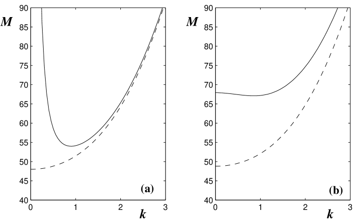
Figure 1: (a) Linear stability curve obtained from the full governing equations without rotation for $Bi_{1}=Bi_{2}=0$ (dashed line) and for $Bi_{1}>0$ and $Bi_{2}>0$ (solid line); (b) Linear stability analysis of the full governing equations for $Bi_{1}=Bi_{2}=0$ at $\Omega=1$ (dashed line) and $\Omega=5$ (solid line).

As shown in Fig.1a the critical wavenumber $q_{c}$ vanishes for $Bi_{1}=Bi_{2}=0$, while for $Bi_{1}>0$ and $Bi_{2}>0$ one has $q_{c}>0$. A series expansion of (20) around $Bi_{1}=Bi_{2}=0$ shows that $q_{c}=((Bi_{1}+Bi_{2})405/27)^{1/4}$. Thus, for poorly conducting boundary conditions the wavenumber of the growing pattern is still small enough to allow the description by a long-wave model. In Fig.1b the marginal curve is shown for $Bi_{1}=Bi_{2}=0$ and two values of the rotation rate, $\Omega=1$ and $\Omega=5$. We see that small values of the rotation rate do not modify the critical wavenumber. However for $\Omega>\Omega_{c}\equiv 3.7513$ a minimum develops in the neutral curve even for $Bi_{1}=Bi_{2}=0$ and the critical wavenumber changes sharply from zero to a finite value. Thus, our study will be valid only for $\Omega<\Omega_{c}$. In this regime the critical Marangoni number at $q=0$ as a function of $\Omega$ is given by

$$M_{c}(\Omega)|_{q=0}={\frac{4\,{\Omega}^{3/2}\left(2\,\cos(\sqrt{\Omega})\sin(\sqrt{\Omega})-\sinh(2\,\sqrt{\Omega})\right)}{4\,\sinh(\sqrt{\Omega})\sin(\sqrt{\Omega})+\cos(2\,\sqrt{\Omega})-\cosh(2\,\sqrt{\Omega})}}.$$ (23)

4 Derivation of the Long-Wave Equation

Here we derive the long-wavelength model for rotating Marangoni convection and consider the system (3)-(10) together with the boundary conditions (14)-(15). Expanding $\theta$ and ${\bf u}$ around the conductive solution, we rewrite the equations in terms of the deviations from the basic solution. To avoid excessive notation we keep the same notation $\theta$ and ${\bf u}$ for deviations of the temperature and velocity fields and obtain

$$\nabla^{4}w-2\Omega\partial_{z}\zeta = 0,$$ (24)

$$\nabla^{2}\zeta+2\Omega\partial_{z}w = 0,$$ (25)

$$\Delta_{H}u+\partial_{x}\partial_{z}w+\partial_{y}\zeta = 0,$$ (26)

$$\Delta_{H}v+\partial_{y}\partial_{z}w-\partial_{x}\zeta = 0,$$ (27)

$$\left(\partial_{t}+{\bf u}\cdot\nabla\right)\theta = w+\Delta\theta.$$ (28)

The boundary conditions are:

$$\theta_{z}-Bi_{1}\theta=w=\zeta=w_{z}=0, {\rm at}\,z=0,$$ (29)

$$w_{zz}-M\Delta_{H}\theta=\theta_{z}+Bi_{2}\theta=w=\zeta_{z}=0, {\rm at}\,z=1.$$ (30)

We define a small parameter $\epsilon$ which measures distance from the critical Marangoni number by setting:

$$M=M_{c}(1+\epsilon^{2}\mu).$$ (31)

Here $\mu$ is a parameter which allows to introduce changes in the Marangoni number independently of $\epsilon$. We assume that the heat loss is small,

$$Bi=\epsilon^{4}b.$$ (32)

As discussed above, this implies that the dimensionless wavelength of the initial instability is long, of order $\epsilon^{-1}$. This allow us to introduce the slow scales,

$$X=\epsilon x,\,\,\,\,\,\,\,Y=\epsilon y.$$ (33)

The vertical coordinate $z$ is not rescaled. The evolution occurs on the slow time $T$,

$$t=\epsilon^{4}T,$$ (34)

as suggested by the linear stability analysis [23]. These scalings of space and time suggest the scaling of the fields involved. Specifically, the Marangoni condition (30) suggests that the vertical velocity be taken to be small while the deviation of the temperature from the linear profile can be large,

$$(w,\theta)=(\epsilon^{2}W,\Theta).$$ (35)

Equations (26) and (27) point out the scaling for the $x$ and $y$ component of the velocity,

$$(u,v)=(\epsilon U,\epsilon V).$$ (36)

From the definition of the $z$-component of the vorticity and considering the previous scaling we have,

$$\zeta=\epsilon^{2}Z.$$ (37)

With these definitions the equations (24)-(28) become:

$${\rm D}^{4}W+2\epsilon^{2}{\rm D}^{2}\Delta_{H}W+\epsilon^{4}\nabla_{H}^{4}-2\Omega{\rm D}Z = 0,$$ (38)

$${\rm D}^{2}Z+2\Omega{\rm D}W+\epsilon^{2}\Delta_{H}Z = 0,$$ (39)

$$\Delta_{H}U+W_{Xz}+Z_{Y} = 0,$$ (40)

$$\Delta_{H}V+W_{Yz}-Z_{X} = 0,$$ (41)

$$\epsilon^{4}\Theta_{T}-{\rm D}^{4}\Theta-\epsilon^{2}\Delta_{H}\Theta-\epsilon^{2}W = -\epsilon^{2}U\Theta_{X}-\epsilon^{2}W\Theta_{Y}-\epsilon^{2}W{\rm D}\Theta,$$ (42)

with D$\equiv\partial/\partial z$. The boundary conditions are,

$$W={\rm D}W=Z={\rm D}\Theta-b_{1}\epsilon^{4}\Theta=0, \,\,{\rm on}\,z=0,$$ (43)

$$W={\rm D}^{2}W-M_{c}(1+\epsilon^{2}\mu)\Delta_{H}\Theta={\rm D}Z={\rm D}\Theta-b_{2}\epsilon^{4}\Theta=0, \,\,{\rm on}\,z=1.$$ (44)

Proceeding as in Refs. [24, 23], we expand the temperature as follows,

$$\Theta=\Theta_{0}(X,Y,z,T)+\epsilon^{2}\Theta_{1}(X,Y,z,T)+...,$$

and similarly for the other fields. Because in (38)-(44) only even powers of $\epsilon$ appear, the expansion of the fields can also be restricted to even powers. If we insert these expansions in (38)-(44) we obtain at ${\mathcal{O}}(\epsilon^{0})$

$$\Theta_{0} = F(X,Y,T),$$ (45)

$$W_{0} = M\,\Delta_{H}F\,f_{1}(\Omega,z),$$ (46)

$$Z_{0} = M\,\Delta_{H}F\,f_{2}(\Omega,z),$$ (47)

$$U_{0} = -M\,(F_{X}\,{\rm D}f_{2}+F_{Y}\,f_{1}),$$ (48)

$$V_{0} = -M\,(F_{Y}\,{\rm D}f_{2}-F_{X}\,f_{1}).$$ (49)

In contrast to the non-rotating case the vertical vorticity $Z$ does not vanish and at each order we must solve two coupled inhomogeneous differential equations instead of only one as in [24]. In these expressions $F(X,Y,T)$ is the planform function whose governing equation we are looking for. The functions $f_{1}$ and $f_{2}$ are complicated functions of $\Omega$ and $z$. In the limit $\Omega\to 0$ the function $f_{2}$ vanishes and $f_{1}$ is the same as in [24].

At ${\mathcal{O}}(\epsilon^{2})$ we obtain,

$${\rm D^{2}}\Theta_{1}=-\Delta_{H}F-M\,f_{1}\,\Delta_{H}F-M\,{\rm D}f_{1}\,|\nabla_{H}F|^{2}.$$

The critical Marangoni number at $k=0$ is obtained from the solvability condition in agreement with the expression (23) obtained in the linear stability analysis. For the fields we obtain

$$\Theta_{1} = f_{3}(\Omega,z)\Delta_{H}F+f_{4}(\Omega,z)|\nabla_{H}F|^{2}+F_{2}(X,Y,T),$$ (50)

$$W_{1} = f_{5}(\Omega,z)\Delta_{H}F+f_{6}(\Omega,z)\Delta_{H}^{2}F+f_{7}(\Omega,z)\Delta_{H}|\nabla_{H}F|^{2}+$$ (51)

$$f_{8}(\Omega,z)\Delta_{H}F_{2},$$

$$Z_{1} = f_{9}(\Omega,z)\Delta_{H}F+f_{10}(\Omega,z)\Delta_{H}^{2}F+f_{11}(\Omega,z)\Delta_{H}|\nabla_{H}F|^{2}+$$ (52)

$$f_{12}(\Omega,z)\Delta_{H}F_{2},$$

$$U_{1} = -f_{9}\,F_{Y}-f_{10}\,\Delta_{H}F_{Y}-f_{11}\,(|\nabla_{H}F|^{2})_{Y}-f_{12}\,F_{2,Y}-f_{5,z}\,F_{X}-$$ (53)

$$f_{6,z}\,\Delta_{H}F_{X}-f_{7,z}(|\nabla_{H}F|^{2})_{X}-f_{8,z}F_{2,X},$$

$$V_{1} = f_{9}\,F_{X}+f_{10}\,\Delta_{H}F_{X}+f_{11}\,(|\nabla_{H}F|^{2})_{X}+f_{12}\,F_{2,X}-f_{5,z}\,F_{Y}-$$ (54)

$$f_{6,z}\,\Delta_{H}F_{Y}-f_{7,z}(|\nabla_{H}F|^{2})_{Y}-f_{8,z}F_{2,Y}.$$

Here $F_{2}$ is the $O(\epsilon^{2})$-correction to the planform function $F$. The functions $f_{3}$, $f_{4}$, $f_{5}$, $f_{6}$, $f_{7}$, $f_{8}$, $f_{9}$, $f_{10}$, $f_{11}$ and $f_{12}$ are again complicated functions of $z$ and $\Omega$. The functions $f_{3}$ and $f_{4}$ are related to integrals of $f_{1}$ with respect to $z$. It turns out that after the integration these functions contain terms that are singular at $\Omega=0$ and do not depend on $z$ in this limit. In order to cancel these singularities and to recover the expressions of [24] in the limit $\Omega\to 0$, the planform function $F_{2}$, which is undetermined at this order, must contain the same singular constants with the opposite sign. Since the integral expressions are too complicate to present here, this is best illustrated by the simple example

$$\int\sin(\Omega z)dz=-\frac{1}{\Omega}\cos(\Omega z)+C.$$ (55)

This integral is not finite in the limit $\Omega\to 0$. If a finite value is required for it, the arbitrary constant $C$ must be chosen as $1/\Omega$. Analogously, in $f_{3}$ and $f_{4}$ constants appear that need to be chosen appropriately. Since they do not depend on $z$ they can be absorbed in $F_{2}$ and therefore do not affect the long-wave equation for $F$.

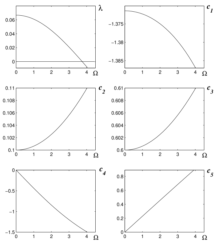
Figure 2: The constants $\lambda$, $c_{1}$, $c_{2}$, $c_{3}$, $c_{4}$ and $c_{5}$ plotted as functions of the rotation rate $\Omega$.

Finally, at ${\mathcal{O}}(\epsilon^{4})$ the solvability condition for D${}^{2}\Theta_{2}$ yields the required equation for the planform function $F(X,Y,T)$,

$$F_{T} = -(b_{1}+b_{2})F-\mu\Delta_{H}F-\lambda\Delta_{H}^{2}F-c_{1}\nabla_{H}\cdot|\nabla_{H}F|^{2}\nabla_{H}F-$$ (56)

$$c_{2}\nabla_{H}\cdot\Delta_{H}F\nabla_{H}F-c_{3}\Delta_{H}|\nabla_{H}F|^{2}-c_{4}{\bf e}_{z}\cdot\nabla_{H}F\times\nabla_{H}\left\{\Delta F\right\}$$

$$+c_{5}{\bf e}_{z}\cdot\nabla_{H}F\times\nabla_{H}\left\{(\nabla_{H}F)^{2}\right\}.$$

Here $\mu$ is the control parameter (cf. (31)) The constants $\lambda$, $c_{1}$, $c_{2}$, $c_{3}$, $c_{4}$ and $c_{5}$ are complicated functions of the rotation rate $\Omega$. We plot them in Fig. 2. A series expansion of these functions around $\Omega=0$, shows that in the limit $\Omega\to 0$, the same equation as in [24] is obtained:

$$\lambda = {\frac{1}{15}}-{\frac{7}{1200}}{\Omega}^{2}+\mathcal{O}\left({\Omega}^{4}\right),$$

$$c_{1} = -{\frac{48}{35}}-{\frac{104}{121275}}{\Omega}^{2}+\mathcal{O}\left({\Omega}^{4}\right),$$

$$c_{2} = {\frac{1}{10}}+{\frac{1}{1575}}{\Omega}^{2}+\mathcal{O}\left({\Omega}^{4}\right),$$

$$c_{3} = {\frac{3}{5}}+{\frac{1}{1575}}{\Omega}^{2}+\mathcal{O}\left({\Omega}^{4}\right),$$

$$c_{4} = -{\frac{233}{525}}\Omega+{\frac{404}{72765}}{\Omega}^{3}+\mathcal{O}\left({\Omega}^{5}\right),$$

$$c_{5} = {\frac{8}{35}}\Omega-{\frac{122}{1576575}}{\Omega}^{3}+\mathcal{O}\left({\Omega}^{5}\right).$$

5 Numerical results

We now turn to the stability and dynamics of hexagon patterns described by (56). One of our goals is to identify parameter regimes in which regular hexagon patterns become unstable at all wavenumbers. In the weakly nonlinear case hexagons can be described by three coupled Ginzburg-Landau equations. Within this framework their stability and dynamics has been studied in detail without and with rotation [43, 44, 45, 46, 31, 32, 47]. It has been found that for small amplitudes there is always a range of wavenumbers over which the hexagons are stable. In a simple Swift-Hohenberg model, situations were identified in which somewhat further above onset the stability balloon closes, leading to persistent chaotic dynamics [34]. In this paper we therefore do not reduce (56) to small-amplitude Ginzburg-Landau equations. Instead determine the stability of the hexagon solutions of (56) and the resulting dynamics numerically without any restriction to small amplitudes.

The stability of the hexagon patterns is determined with a Fourier-Galerkin code on a hexagonal lattice. We then determine their stability with respect to side-band perturbations using a Floquet analysis with a Floquet parameter ${\bf p}=p(\cos\theta,\sin\theta)$. Due to the isotropy of the system and the discrete rotational symmetry of the hexagons we can restrict our analysis to perturbation wavevectors subtending an angle $\theta$ of up to $\pm 30^{o}$ relative to the hexagon modes. It turns out that accurate solutions of (56) require a large number of Fourier modes. One measure of the accuracy of a solution is obtained with the stability analysis by determining the magnitude of the eigenvalue corresponding to the translation mode given by the Floquet parameter ${\bf p}=0$. For the exact solution one has $\sigma({\bf p})=0$, while numerically truncated solutions will have $\sigma({\bf p})\neq 0$. The dependence of $\sigma({\bf p})$ as a function of the number $n$ of harmonics retained is illustrated in table 1, where $n=1$ corresponds to the basic hexagon solution.

$\mu$	$\Omega$	q	$n=7$	$n=11$	$n=15$
$0.07$	$3.0$	$0.98$	$-0.16\cdot 10^{-3}$	$-0.28\cdot 10^{-5}$	$-0.56\cdot 10^{-7}$
$0.17$	$2.5$	$0.95$	$-0.25\cdot 10^{-1}$	$-0.53\cdot 10^{-2}$	$-0.60\cdot 10^{-3}$

Table 1: Translation eigenvalue $\sigma({\bf p}=0)$ as a function of the truncation parameter $n$ of the Fourier expansion for $b_{1}+b_{2}=0.025$ illustrating the poor convergence for larger amplitudes.

Fig.3 shows the resulting stability limits in the absence of rotation ($\Omega=0$) for $b_{1}+b_{2}=0.025$. They are given by steady long-wave instabilities with $p\ll 1$ (cf.[43, 44, 47]). Numerical simulations for selected parameter values (marked by plusses and crosses in fig.3) confirm that the instabilities lead to the formation of defects which then change the wavevector of the pattern.

Figure 3: Stability limits of the steady hexagons for $\Omega=0$ and $b_{1}+b_{2}=0.025$. The dashed line gives the neutral curve. The stability limit is given by a steady long-wave instability (solid line). The plusses and crosses indicate stable and unstable solutions according to the numerical simulation.

Rotation strongly modifies the stability limits as shown in fig.4 for $\Omega=3$ and $b_{1}+b_{2}=0.025$. The most striking aspect is that the stability balloon closes for $\mu>0.07$. This closing is due to a steady short-wave instability (triangles) which supersedes the usual steady long-wave instability (open circles) for larger $\mu$. In the short-wave regime the largest growth rates are obtained for $p\approx 0.6q$ and $\theta\approx 25^{o}-30^{o}$. The appearance of a short-wave instability is somewhat similar to the result found in the weakly nonlinear analysis. There it has been found that in the presence of rotation a steady or oscillatory instability arises at finite modulation wavenumbers and preempts the long-wave oscillatory instability that emerges from the interaction of the two long-wave phase modes [31].

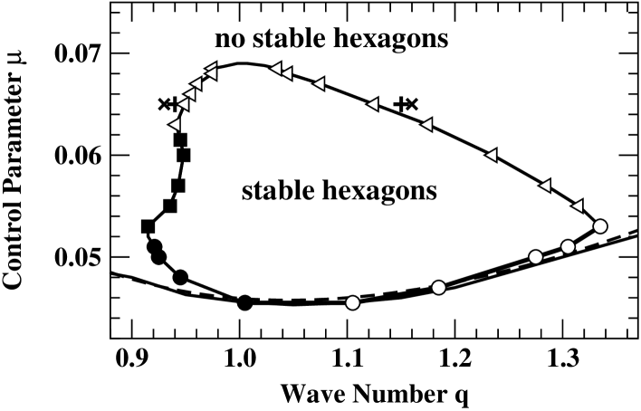
Figure 4: Stability limits of the steady hexagons for $\Omega=3$ and $b_{1}+b_{2}=0.025$. Hexagons are only stable inside the closed loop. The neutral and saddle-node lines are given by thin dashed and solid lines. The symbols identify the character of the relevant instabilities: long-wave steady (open circles), short-wave steady (open left-triangles), long-wave oscillatory (solid circles), homogeneously oscillatory (solid squares). The plusses and crosses denote simulations in which the steady hexagons were stable/unstable (see text).

A further interesting feature of the stability limits for $\Omega=3$ is the oscillatory instability that limits the stability balloon on the low-$q$ side (solid symbols). For low values of $\mu$ it is a long-wave side-band instability, i.e. its growth rate and frequency vanish for ${\bf p}=0$ (solid circles). For larger $\mu$, however, the largest growth rate occurs at ${\bf p}=0$ and the hexagon pattern is unstable to a homogeneous oscillatory mode (solid squares). In the weakly nonlinear analysis such a homogeneous oscillatory instability has only been identified in the context of the transition from hexagons to rolls [26, 27, 31]. No such connection is apparent in the present system.

Anticipating interesting dynamics for values of $\mu$ above the closing of the stability balloon, we have studied its dependence on the rotation rate. As a function of $\Omega$, fig.5 shows the maximal control parameter $\mu$ for which there are still stable steady hexagons (solid squares). To indicate the $\mu$-range of stable hexagons the critical control parameter $\mu_{c}$ is also given (dashed line). With decreasing $\Omega$ that $\mu$-range grows rapidly. To resolve the stability limits for yet smaller values of $\Omega$ a very large number of modes is needed; $n=19$ is not sufficient (cf. table 1).

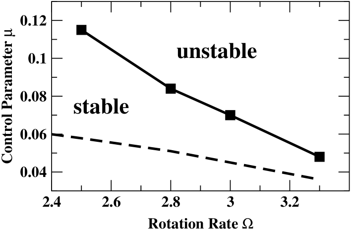
Figure 5: Maximal value of the control parameter for which there are still steady hexagons (solid line) and onset of hexagons (dashed line) ($b_{1}+b_{2}=0.025$).

The nonlinear evolution ensuing from the linear instabilities is investigated by simulating (56) numerically with a pseudo-spectral Fourier code using an integrating-factor, fourth-order Runge-Kutta scheme. It turns out that for larger values of $\mu$ the nonlinear gradient terms in (56) can under certain conditions lead to an apparently spurious blow-up of the numerical solution in which very high wavenumbers are excited [48]. However, if a sufficiently smooth initial condition was used no such numerical divergencies occurred. As already indicated earlier (cf. table 1) the proper resolution of the patterns requires a large number of Fourier modes. In all simulations we have used a rectangular computational domain of size $L_{X}=2L$ and $L_{Y}=2L/\sqrt{3}$ to accommodate undeformed hexagon patterns. Specifically, for $L=N\,2\pi/q$ this domain allows $N$ periods of the pattern in the $x$- and $y$-direction.

To test the stability results we have performed simulations near the stability limits depicted in figs.3,4. The plusses denote parameters for which a small modulation of the pattern did not destabilize it, while at the crosses the hexagons became unstable. These simulations were performed in systems of size $L=4\cdot 2\pi/q$. For this aspect ratio some of the instabilities are still slightly suppressed shifting the stability limits somewhat. The limits obtained in the simulations are, however, consistent with the stability results if the modulation wavenumbers ${\bf p}$ are restricted to those compatible with the computational domain used in the simulations.

We first address the nonlinear evolution of the homogeneous oscillatory instability (solid squares). Simulations for $\mu=0.060$ and $q=0.93$ show that this stability limit is due to a supercritical Hopf bifurcation, i.e. the spatially homogeneous oscillations saturate and lead to a state of oscillating hexagons. They are similar in appearance to the oscillating hexagons that arise in the Hopf bifurcation that replaces the instability of hexagons to the mixed mode, which is associated with the transition to rolls. As mentioned earlier, this transition to the mixed mode and to rolls has not been seen in the present system. A time sequence of snapshots of the oscillating hexagons is shown in fig.6.

see figures homosz.0149.c.jpg homosz.0156.c.jpg homosz.0159.c.jpg homosz.0163.c.jpg

Figure 6: Snapshots of oscillating hexagons for $\Omega=3$ and $b_{1}+b_{2}=0.025$, $\mu=0.060$, and $q=0.93$ at times $t=0$, $t=\frac{1}{3}T$, $t=0.43T$, and $t=\frac{2}{3}T$, where the period $T=140$ (time progressing left to right, top to bottom; red denotes positive, blue negative values).

Now we turn to the nonlinear evolution arising from the steady short-wave instability (open left-triangles in fig.4). In fig.7 and fig.8 a sequence of the pattern and the temporal evolution of two modes is shown, respectively in a system of size $L_{X}=20.8$ for $\mu=0.07$ (using $128\times 128$ modes). For this value of the control parameter no stable hexagon patterns exist in the infinite system. In this case the temporal evolution does not become periodic for the time period investigated.

see fig7artc.jpg

Figure 7: Snapshots of typical patterns obtained for $\Omega=3$ and $b_{1}+b_{2}=0.025$ at $L_{X}=20.8,\mu=0.07$ at times 6299, 6349, 6449, 6499, 6549, 6599, 6649, 6749 (left to right and top to bottom)

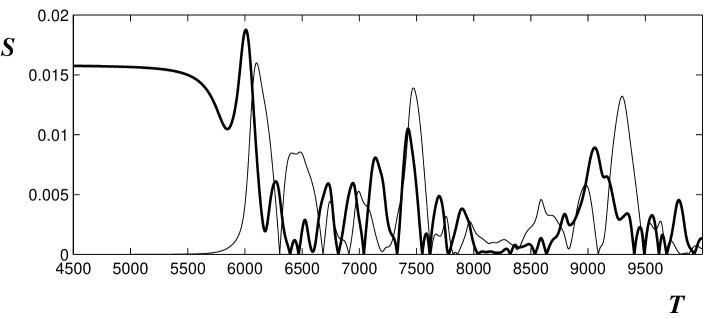
Figure 8: Time series obtained for $\Omega=3$ and $b_{1}+b_{2}=0.025$ at $L_{X}=20.8$, $\mu=0.07$. It shows the energy $S$ associated with the Fourier modes with wavevectors $(2\pi/20.8,2\cdot 2\pi\sqrt{3}/20.8)$ with thin and thick solid lines, respectively. Note the long onset time for the instability.

In fig.9 typical snapshots for the evolution of the pattern in a system of size $L_{X}=48$ are shown for $\mu=0.08$ (using $256\times 256$ modes). The associated time series for two Fourier modes are shown in fig.10. Again, for these parameter values no steady stable hexagons exist in large systems resulting in persistent chaotic dynamics. While the pattern is spatially quite disordered a tendency to form locally square arrangements can be observed. This presumably reflects the fact that in the absence of the quadratic terms in (56) even in the rotating system square patterns are preferred over roll patterns [35].

fig9artc.jpg

Figure 9: Typical patterns obtained for $\Omega=3$ and $b_{1}+b_{2}=0.025$ at $L_{X}=48,\mu=0.08$ at times 2699, 3749, 3899, 11549 (left to right and top to bottom).

see fig10.jpg

Figure 10: Time series obtained for $\Omega=3$ and $b_{1}+b_{2}=0.025$ at $L_{X}=48,\mu=0.08$. The energy $S$ associated with the amplitude of the Fourier modes with wavevector $(2\cdot 2\pi/48,4\cdot 2\pi\sqrt{3}/48)$ and $(0,4\cdot 2\pi\sqrt{3}/48)$ are shown with thin and thick solid lines, respectively.

see fig11artc.jpg

Figure 11: Patterns in a cycle obtained for $\Omega=3$ and $b_{1}+b_{2}=0.025$ at $L_{X}=17$, $\mu=0.058$ at times 4079.2, 4159.2, 4239.2, 4319.2, 4399.2, 4479.2, 4559.2, 4639.2 (left to right and top to bottom).

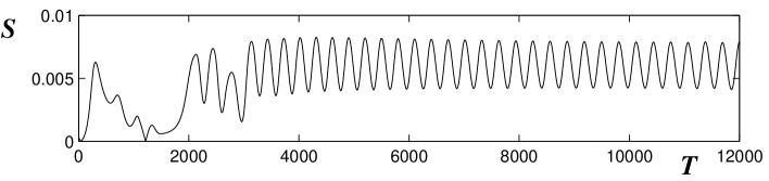
Figure 12: Time series obtained for $\Omega=3$ and $b_{1}+b_{2}=0.025$ at $L_{X}=17$, $\mu=0.058$. It shows the energy $S$ associated with the Fourier mode with wavevector $(2\pi/17,2\cdot 2\pi\sqrt{3}/17)$.

Finally, in Figs.11, 12 we show the temporal evolution in a quite small system of size $L_{X}=17$ for $\mu=0.058$ (using $64\times 64$ Fourier modes). For such a small system the stability limits as shown in figs.4 do not really apply. The initial condition was a regular hexagon pattern with wavenumber $q=1.478$. After a transient during which defects appeared and changed the number of cells the time dependence of the pattern becomes quite regular. The time series (cf. fig.12) is, however, not strictly periodic but shows small ($\approx 1\%$) irregular variations of the oscillation amplitude. A closer inspection of the neutral curve, which in terms of the system size and of the number $N$ of wavelengths contained in the system is given by

$$\mu(L_{x})=b\left(\frac{L_{X}}{4\pi N}\right)^{2}+\lambda\left(\frac{4\pi N}{L_{X}}\right)^{2},$$ (57)

shows that the parameters for this simulation are close to the codimension-two point at which hexagons with $q=0.74$ and hexagons with $q=1.48$ first arise. This is illustrated in fig.13 which gives the neutral curve (57) for various values of $N$. In this small system we associate the origin of the dynamics with the low-dimensional interaction of the two modes associated with the codimension-two point.

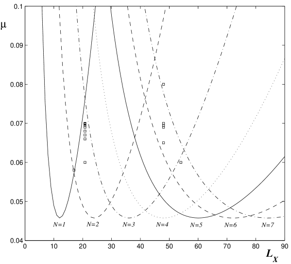
Figure 13: The neutral curve $\mu(L_{X})$ plotted for different values of $N$, the number of wavelengths contained in the system. The parameters are $b_{1}+b_{2}=0.025$ and $\lambda=0.0209$ (which corresponds to a rotation rate of $\Omega=3$). Squares stand for numerical simulations performed in different boxes at different $\mu$ values.

6 Conclusion

In this paper we have considered Marangoni convection in the presence of rotation. In order to derive systematically a set of reduced equations that - unlike the Ginzburg-Landau equations - preserve the isotropy of the system we have considered poorly conducting boundary conditions. Under these conditions convection sets in first at long wavelengths, which allows the derivation of a long-wave equation. Extending previous analyses [24, 49], we have derived the long-wave equation in the presence of rotation and obtained the coefficients as a function of the rotation rate $\Omega$. Using a Galerkin approach we have then determined the linear stability of steady hexagonal convection with respect to general side-band perturbations without and with rotation. We have employed direct numerical simulations of the long-wave equation to investigate the fate of these instabilities.

In the absence of rotation the band of stable steady hexagons in large systems is determined solely by a steady long-wave instability for the range of the control parameter considered. With rotation, however, steady long- and short-wave instabilities as well as oscillatory instabilities arise. The latter can be a long-wave side-band instability or an instability that is spatially homogeneous at its onset. Interestingly, the latter is supercritical and leads to stable, spatially homogeneous oscillations of the hexagons. This state resembles the oscillating-hexagon branch that arises in non-Boussinesq buoyancy-driven convection in connection with the transition from hexagon to roll convection [26, 27, 31]. In the present system no transition to rolls has been identified and in experiments on Marangoni convection a transition from hexagons to squares is observed instead [17, 19]. We find temporally almost periodic and spatially more complex states that appear to arise from a resonant $q:2q$ mode interaction. This and other resonances could be studied in future work. Most interesting is the fact that for sufficiently large rotation rates the stability limits close for larger values of the control parameter. In the numerical simulations this is shown to lead to spatially and temporally chaotic patterns.

So far, there have been very few experimental studies of spatio-temporal chaos arising from a hexagonal planform [50]. Therefore, it would be particularly interesting to see whether the complex dynamics of the disordered hexagonal patterns predicted by the long-wave model (56) can be obtained in experiments. It is yet to be seen to what extent in the current system the deformation of the free surface by the centrifugal force modifies the results presented here. Similarly, the derivation of the long-wave equation depends on the poor thermal conductivity of the horizontal boundaries. For experimentally realizable boundary conditions the wavelength of the convecting state may not be as large [14]. As is often the case, however, the instabilities predicted by the long-wave equation (56) may persist qualitatively beyond the asymptotic long-wave limit. A study of this question will presumably require the derivation of the Ginzburg-Landau equations with nonlinear gradient terms or, more likely due to the finite amplitudes at the closing of the stability balloon, a numerical analysis of the full fluid equations (cf.[16]).

References

- [1] G. Küppers and D. Lortz. Transition from laminar convection to thermal turbulence in a rotating fluid layer. J. Fluid Mech., 35:609, 1969.
- [2] F.H. Busse and R.M. Clever. Nonstationary convection in a rotating system. In U. Müller, K.G. Roesner, and B. Schmidt, editors, Recent developments in theoretical and experimental fluid mechanics, page 376, Berlin, 1979. Springer.
- [3] F.H. Busse and K.E. Heikes. Convection in a rotating layer: a simple case of turbulence. Science, 208:173, 1980.
- [4] F. Zhong, R. Ecke, and V. Steinberg. Rotating Rayleigh-Bénard convection: the Küppers-Lortz transition. Physica D, 51:596, 1991.
- [5] Y. Hu, W. Pesch, G. Ahlers, and R. E. Ecke. Convection under rotation for Prandtl numbers near one: Küppers-Lortz instability. Phys. Rev. E, 58:5821, 1998.
- [6] M.C. Cross, D. Meiron, and Y. Tu. Chaotic domains: a numerical investigation. Chaos, 4:607, 1994.
- [7] M. F. Schatz and G. P. Neitzel. Experiments on thermocapillary instabilities. Ann. Rev. Fluid Mech., 33(6):93, June 2001.
- [8] J.R.A. Pearson. On convective cells induced by surface tension. J. Fluid Mech., 4:489, 1958.
- [9] L.E. Scriven and C.V. Sternling. On celular convection driven by surface-tension gradients: effects of mean surface tension and surface viscosity. J. Fluid Mech., 19:321, 1964.
- [10] K.A. Smith. On convective instability induced by surface-tension gradients. J. Fluid Mech., 24:401, 1966.
- [11] A. Juel, J. M. Burgess, W.D. McCormick, J.B. Swift, and Harry L. Swinney. Surface tension-driven convection patterns in two liquid layers. Physica D, 143:169, 2000.
- [12] A. Engel and J. B. Swift. Planform selection in two-layer Bénard-Marangoni convection. Phys. Rev. E, 62(5):6540–6553, November 2000.
- [13] S.J. VanHook, M.F. Schatz, W.D. McCormick, J.B. Swift, and H.L. Swinney. Long-wavelength instability in surface-tension-driven Bénard convection. Phys. Rev. Lett., 75:4397, 1995.
- [14] S.J. VanHook, M.F. Schatz, J.B. Swift, W.D. McCormick, and H.L. Swinney. Long-wavelength surface-tension-driven Bénard convection: experiment and theory. J. Fluid Mech., 345:45–78, 1997.
- [15] B. Echebarria and C. Pérez-Garcia. Stability of hexagonal patterns in Bénard-Marangoni convection. Phys. Rev. E, 63(6):066307, June 2001.
- [16] M. Bestehorn. Phase and amplitude instabilities for Bénard-Marangoni convection in fluid layers with large aspect ratio. Phys. Rev. E, 48:3622, 1993.
- [17] K. Nitschke and A. Thess. Secondary instability in surface-tension-driven Bénard convection. Phys. Rev. E, 52:5772, 1995.
- [18] K. Eckert, M. Bestehorn, and A. Thess. Square cells in surface-tension-driven Bénard convection: Experiment and theory. J. Fluid Mech., 356(2):155–197, February 1998.
- [19] M. F. Schatz, S. J. VanHook, W. D. McCormick, J. B. Swift, and H. L. Swinney. Time-independent square patterns in surface-tension-driven Bénard convection. Phys. Fluids, 11(9):2577–2582, September 1999.
- [20] W. A. Tokaruk, T. C. A. Molteno, and S. W. Morris. Bénard-Marangoni convection in two-layered liquids. Phys. Rev. Lett., 84:3590, 2000.
- [21] A.A. Golovin, A.A. Nepomnyashchy, and L.M. Pismen. Interaction between short-scale Marangoni convection and long-scale deformational instability. Phys. Fluids, 6:34, 1994.
- [22] A.A. Golovin, A.A. Nepomnyashchy, L.M. Pismen, and H. Riecke. Steady and oscillatory side-band instabilities in Marangoni convection with deformable interface. Physica D, 106:131–147, 1997.
- [23] G. Sivashinsky. Large cells in nonlinear Marangoni convection. Physica D, 4:227, 1982.
- [24] E. Knobloch. Pattern selection in long-wavelength convection. Physica D, 41:450, 1990.
- [25] A. A. Golovin, A. A. Nepomnyashchy, and L. M. Pismen. Pattern-formation in large-scale Marangoni convection with deformable interface. Physica D, 81(1-2):117–147, February 1995.
- [26] J.W. Swift. Convection in a rotating fluid layer. In Contemporary Mathematics Vol. 28, page 435, Providence, 1984. American Mathematical Society.
- [27] A.M. Soward. Bifurcation and stability of finite amplitude convection in a rotating layer. Physica D, 14:227–241, 1985.
- [28] H. F. Goldstein, E. Knobloch, and M. Silber. Planform selection in rotating convection - hexagonal symmetry. Phys. Rev. A, 46(8):4755–4761, October 1992.
- [29] D.N. Riahi. Nonlinear Bénard-Marangoni convection in a rotating layer. Int. J. Eng. Sci., 32:877, 1994.
- [30] J. Millán-Rodríguez, C. Perez-Garcia, M. Bestehorn, M. Fantz, and R. Friedrich. Pattern formation in convection of rotating fluids with broken vertical symmetry. Phys. Rev. A, 46:4729, 1992.
- [31] B. Echebarria and H. Riecke. Instabilities of hexagonal patterns with broken chiral symmetry. Physica D, 139:97–108, 2000.
- [32] B. Echebarria and H. Riecke. Defect chaos of oscillating hexagons in rotating convection. Phys. Rev. Lett., 84:4838, 2000.
- [33] B. Echebarria and H. Riecke. Stability of oscillating hexagons in rotating convection. Physica D, 143:187, 2000.
- [34] F. Sain and H. Riecke. Instabilities and spatio-temporal chaos of hexagonal patterns with broken chiral symmetry. Physica D, 144:124, 2000.
- [35] S.M. Cox. Long-wavelength rotating convection between poorly conducting boundaries. SIAM J. Appl. Math., 58:1338, 1998.
- [36] E. Knobloch. Pattern selection in binary-fluid convection at positive separation ratios. Phys. Rev. A, 40(3):1549–1559, August 1989.
- [37] F. Marqués, M. Net, J.M. Massaguer, and I. Mercader. Thermal-convection in vertical cylinders - a method based on potentials of velocity. Computer Methods in Applied Mechanics and Engineering, 110:157, 1993.
- [38] A. Vidal and A. Acrivos. The influence of Coriolis force on surface-tension-driven convection. J. Fluid Mech., 26:807, 1966.
- [39] A. Kaddame and G. Lebon. Bénard-Marangoni convection in a rotating fluid with and without surface deformation. Appl. Sci. Res., 52:295, 1994.
- [40] J.J. Jou, K.Y. Kung, and C.H. Hsu. Effects of Coriolis force and surface tension on Bénard-Marangoni convective instability. Int. J. Heat Mass Transfer, 40:1447, 1997.
- [41] A.A. Golovin, A.A. Nepomnyashchy, and L.M. Pismen. Pattern formation in large-scale Marangoni convection with deformable interface. Physica D, 81:117–147, 1995.
- [42] G.A. McConaghy and B.A. Finlayson. Surface tension driven oscillatory instability in a rotating fluid layer. J. Fluid Mech., 39:49, 1969.
- [43] J. Lauzeral, S. Metens, and D. Walgraef. On the phase dynamics of hexagonal patterns. Europhys. Lett., 24:707, 1993.
- [44] M.M. Sushchik and L.S. Tsimring. The Eckhaus instability in hexagonal patterns. Physica D, 74:90, 1994.
- [45] B. Echebarria and C. Pérez-García. Phase instabilities in hexagonal patterns. Europhys. Lett., 43:35, 1998.
- [46] A.E. Nuz, A.A. Nepomnyashchy, A.A. Golovin, A.A. Hari, and L.M. Pismen. Stability of rolls and hexagonal patterns in non-potential systems. Physica D, 135:233–262, 2000.
- [47] Y. Young and H. Riecke. Mean flow in hexagonal convection: stability and nonlinear dynamics. Physica D, 2002.
- [48] F. Sain. Instabilities and Spatio-Temporal chaos of hexagons in the presence of rotation. PhD thesis, Northwestern University, 2000.
- [49] L. Shtilman and G. Sivashinsky. Hexagonal structure of large-scale Marangoni convection. Physica D, 52:477, 1991.
- [50] Q. Ouyang and H.L. Swinney. Transition to chemical turbulence. Chaos, 1:411, 1991.