Comment on “Analysis of chaotic motion and its shape dependence in a generalized piecewise linear map”

Abstract

Rajagopalan and Sabir [Phys. Rev. E 63, 057201 (2001)] recently discussed deterministic diffusion in a piecewise linear map using an approach developed by Fujisaka et al. We first show that they rederived the random walk formula for the diffusion coefficient, which is known to be the exact result for maps of Bernoulli type since the work of Fujisaka and Grossmann [Z. Physik B 48, 261 (1982)]. However, this correct solution is at variance to the diffusion coefficient curve presented in their paper. Referring to another existing approach based on Markov partitions, we answer the question posed by the authors regarding solutions for more general parameter values by recalling the finding of a fractal diffusion coefficient. We finally argue that their model is not suitable for studying intermittent behavior, in contrast to what was suggested in their paper.

The study of deterministic diffusion in simple chaotic maps on the line appears to have originated about twenty years ago (see, e.g., Ref. [3] and further references therein). Already in the seminal work by Fujisaka and Grossmann [4], a variety of piecewise linear models was defined and analyzed by means of stochastic modeling. All these maps are of the form $x_{n+1}=M_{h}(x_{n})$, where $h\in N$ is a control parameter, and $x_{n}$ is the position of a point particle at discrete time $n$. $M_{h}(x)$ is continued periodically beyond the interval $[0,1)$ onto the real line by a lift of degree one, $M_{h}(x+1)=M_{h}(x)+1$. The map defined in Ref. [5], which is sketched again in Fig. 1, provides a straightforward generalization of the one introduced in Ref. [6], which is recovered at $h=1/2$. For this type of maps, indeed a vast literature exists on how to obtain exact analytical results at specific cases of parameter values; Refs. [3, 7] sumarize some of these methods, with more complete lists of references therein. It is furthermore well-known that the calculations are particularly simple if the parameter is such that the map exhibits the Bernoulli property [8].

We first wish to present a considerable shortcut to the diffusion coefficient calculations published in Ref. [5]. Based on a theory which appears to be a precursor of what was called “Fujisaka’s characteristic function method” in Ref. [5], Fujisaka and Grossmann have shown [4] that the diffusion coefficient formula

$$D=\frac{<j^{2}(x_{n})>}{2}$$ (1)

provides the exact solution for types of maps as the one studied in Ref. [5], i.e., if they share the Bernoulli property. Here $j(x_{n})$ is the jump velocity defined as $j(x_{n}):=[x_{n+1}]-[x_{n}]$ with $[x]$ being the largest integer less than $x$, and $<\ldots>$ denotes the average over the invariant probability density. This expression is just identical to the familiar random walk formula for diffusion on a one-dimensional lattice, where the length of jumps squared is weighted with the probability to perform such jumps (see Ref. [9] and further references therein). Evaluating this equation for the map under consideration leads to

$$D(h,r)=\sum_{j=1}^{h}j^{2}\delta(j,r)$$ (2)

with $h\in N,0<r<1$, where $2\delta(j,r)$ denotes the probability to jump over a distance of $j$ steps and is easily calculated to

$$\delta(j,r)=\frac{2}{m_{j}}\;,$$ (3)

$m_{j}$ being the slopes of the map. Combining the above two equations yields Eq. (17) of Ref. [5]. We conclude that Rajagopalan and Sabir have confirmed again Eq. (1) of Fujisaka and Grossmann as applied to their specific map. We now focus on the author’s special case of the map defined by the relation for the slopes

$$m_{0}=3+\frac{4(1-r^{h})}{r^{h}(1-r)}$$ (4)

with $m_{i}/m_{i-1}=r$. Solutions for Eqs. (2), (3) under this constraint are shown in Fig. 2 for different $h$. This figure corrects the erroneous result shown in Fig. 3 of Ref. [5], which only includes a few data points and appears to indicate a rather irregular curve for the diffusion coefficient at $h=2$. Below we will explain why all the curves shown in Fig. 2 must indeed be simple functions of $r$.

However, first we would like to recall a second method which is not restricted to special cases of parameters such as integer heights, in contrast to the one outlined in Refs. [4, 5]. The basic idea of this method is to directly solve the Frobenius-Perron equation of the dynamical system,

$$\rho_{n+1}(x)=\int dy\;\rho_{n}(y)\;\delta(x-M_{h}(y))\;,$$ (5)

where $\rho_{n}(x)$ is the probability density for points on the real line. There exists a dense set of parameter values $h$ for which one can construct Markov partitions of the map, and for each of these parameter values this equation can be written as a matrix equation [3, 10],

$$\mbox{\boldmath$\rho$}_{n+1}=\,T(h,r)\,\mbox{\boldmath$\rho$}_{n}\;.$$ (6)

$\mbox{\boldmath$\rho$}_{n}$ represents a column vector of the probability densities defined on each part of the Markov partition at time $n$, and $T(h,r)$ is a topological transition matrix which can be constructed from the Markov partition. This setup provides two ways of solution: one way is to solve the eigenvalue problem of $T(h,r)$ and to relate the diffusion coefficient to its eigenvalues. As is shown in detail in Refs. [10], in special cases all calculations can be performed analytically. For the simple map defined in Ref. [5] these calculations are straightforward and confirm again Eqs. (2), (3). For more general cases, the matrix equation can simply be iterated [3, 9] yielding numerically exact solutions for the probability density vector $\mbox{\boldmath$\rho$}_{n}$ at any time step $n$, as well as for any other dynamical quantity based on probability density averages. Both such methods were previously applied to various examples of piecewise linear maps [3, 9, 10]. Fig. 1 presents analogous results for the map studied in Ref. [5] at $h=2$ and $r=0.5$, cp. to Fig. 3.1 on p.54 of Ref. [3]. The probability density is a Gaussian on a coarse scale, whereas the fine scale is determined by the invariant density of the map on the unit interval. These deviations from an exact Gaussian can quantitatively be evaluated, e.g., by calculating the curtosis of the respective map density; for a more detailed discussion of such aspects we refer to Chapter 3 of Ref. [3]. This interplay between fine and coarse structure of the probability densities was furthermore discussed in terms of the spectrum of eigenmodes of the Frobenius-Perron operator, see [3, 10]. These known results appear to be recovered in Ref. [5] by a respective analysis of the fluctuation spectrum, which provides an alternative way to look at the probability density of the map.

In their outlook to further work, the authors of Ref. [5] raised the question of how to compute the diffusion coefficient for maps with fractional heights $h$, and how it may look like. The application of the arsenal of methods outlined above has already given a full answer to this problem. As a central result, it was found that the diffusion coefficient for these maps is a fractal function of the parameter $h$. To present an example, Fig. 3 depicts the result for a mirrored zigzag-map with uniform slope, which has some similarities with the one studied in Ref. [5]; for details see Refs. [3, 9]. Knowing these results, it is straightforward to conclude that, for arbitrary height $h$, the map studied in Ref. [5] will just yield another fractal diffusion coefficient; further evidence for that statement is provided by the numerical and analytical data presented in Ref. [11].

So why can the diffusion coefficient of the map in Ref. [5] not be fractal as a function of $r$ at integer values of the height? One way to look at this problem is to inquire how the topology of the map is affected by parameter variation. A fundamental tool providing detailed information about the topology of a dynamical system are Markov partitions. Varying $r$ at integer heights does not change the Markov partition, thus the topology of the map does not change, and any quantity resulting from an average over the invariant density is a simple function of the parameter [12]. However, changing the height changes the Markov partition in a complicated way and reflects the topological instability of the map under this type of parameter variation. This topological instability results in fractal transport coefficients.

Finally, we comment on the conclusion of Rajagopalan and Sabir that the map studied in their paper is “suited in describing diffusion systems showing intermittency”. In this aspect the authors appear to follow Ref. [6], where the map shown in Fig. 1 at $h=1/2$ was introduced for the purpose of modeling “strong correlations between successive steps… as realized in Brownian motion with directional persistence”. Indeed, Grossmann and Thomae revealed a persistent dynamics which they characterized as “intermittent-like” behavior. They linked these correlations to deviations from a pure Gaussian probability density such as the ones discussed above.

In the following we use the term “intermittency” in the sense of Pomeau and Manneville (see, e.g., Ref. [8] for a tutorial about their results). Particularly, we wish to distinguish it from the denotation “intermittency-like” in the sense of Grossmann and Thomae. Extensive studies of diffusion in one-dimensional intermittent maps led to the conclusion that, generally, in this case a diffusion coefficient does not exist [13]. Furthermore, all maps studied in these references are inherently nonlinear. For piecewise linear expanding maps which are uniquely ergodic if restricted to compact spaces, such as the one of Refs. [5, 6], there is no evidence for intermittency nor for anomalous diffusion [3]. Applying the concept of conjugacy enables to transform piecewise linear maps onto nonlinear ones. However, the diffusive dynamics is invariant under conjugacy [6], thus the corresponding nonlinear map is again non-intermittent and normal diffusive. To our knowledge the only piecewise linear map exhibiting intermittency was introduced in Ref. [14], and it belongs to a very different class than the one of Refs. [5, 6].

In summary, by relating the piecewise linear map studied in Ref. [5] to intermittent behavior the authors confuse the meaning of intermittency, in the sense of Pomeau and Manneville, with the existence of intermittent-like behavior, in the sense of persistence in the diffusive motion. Intermittency generally leads to anomalous diffusion, whereas persistence in piecewise linear maps shows up in form of local extrema of the fractal diffusion coefficient at integer and half-integer heights, see Fig. 3. We conclude that the analysis of chaotic motion and its shape dependence as performed in Ref. [5] has nothing to do with intermittency, but instead recovers features of the parameter-dependent normal diffusion coefficient as studied in Refs. [3, 4, 6, 7, 8, 9, 10, 11, 12].

The author thanks N.Korabel and J.R.Dorfman for helpful remarks.

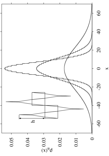
FIG. 1.: Time-dependent probability density $\rho_{n}(x)$ for the map sketched in the figure as it evolves starting from a uniform density in a box situated around $x=0$. The results have been obtained from iterating transition matrices as explained in the text. Included are Gaussian solutions from the ordinary diffusion equation corresponding to the exact diffusion coefficient $D(h,r)$ of the map, where $h=2,r=0.5$. These dashed lines are almost indistinguishable from the map densities, however, they are lacking the step-like fine structure. From above to below, the time steps are $n=20$, $n=50$, $n=200$. The quantities plotted in this and in the following figures are dimensionless.

FIG. 2.: The diffusion coefficient $D(h,r)$ for the map shown in Fig. 1 according to Eqs. (2), (3). Solutions are shown for the values of the height $h=2,3,4,5$ starting from below. The case $h=2$ corrects the erroneous result in Fig. 3 of Ref. [3].

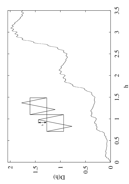
FIG. 3.: Fractal diffusion coefficient $D(h)$ for the mirrored zigzag-map sketched in the figure as a function of the height $h$. Shown are 13376 data points. The data is from Refs. [1,5].

REFERENCES

- [1]
- [2] Electronic address: rklages@mpipks-dresden.mpg.de.
- [3] R. Klages, Deterministic diffusion in one-dimensional chaotic dynamical systems (Wissenschaft & Technik-Verlag, Berlin, 1996).
- [4] H. Fujisaka and S. Grossmann, Z. Physik B 48, 261 (1982).
- [5] S. Rajagopalan and M. Sabir, Phys. Rev. E 63, 057201 (2001).
- [6] S. Grossmann and S. Thomae, Phys. Lett. A 97, 263 (1983).
- [7] P. Gaspard, Chaos, Scattering, and Statistical Mechanics (Cambridge University Press, Cambridge, 1998); J.R. Dorfman, An Introduction to Chaos in Nonequilibrium Statistical Mechanics (Cambridge University Press, Cambridge, 1999); R. Artuso, Classical and quantum zeta-functions and periodic orbit theory; in: G. Casati, I. Guarneri, and U. Smilansky, Editors, New Directions in Quantum Chaos, (IOS Press, Amsterdam, 2000); P. Cvitanović et al., Classical and Quantum Chaos (Niels Bohr Institute, Copenhagen, 2001).
- [8] H.G. Schuster, Deterministic Chaos, 2nd ed. (VCH Verlagsgesellschaft mbH, Weinheim, 1989).
- [9] R. Klages and J.R. Dorfman, Phys. Rev. E 55, R1247 (1997).
- [10] R. Klages and J.R. Dorfman, Phys. Rev. Lett. 74, 387 (1995); Phys. Rev. E 59, 5361 (1999); P. Gaspard and R. Klages, Chaos 8, 409 (1998).
- [11] H.-C. Tseng et al., Phys. Lett. A 195, 74 (1994).
- [12] R. Stoop and W.-H. Steeb, Phys. Rev. E 55, 7763 (1997).
- [13] T. Geisel and S. Thomae, Phys. Rev. Lett. 52, 1936 (1984); T. Geisel, J. Nierwetberg, and A. Zacherl, Phys. Rev. Lett. 54, 616 (1985); R. Artuso, G. Casati, and R. Lombardi, Phys. Rev. Lett. 71, 62 (1993); X.-J. Wang and C.-K. Hu, Phys. Rev. E 48, 728 (1993).
- [14] P. Gaspard and X.-J. Wang, Proc. Nat. Acad. Sci. USA 85, 4591 (1988).