Inverse cascade in Charney-Hasegawa-Mima turbulence

Abstract

The inverse energy cascade in Charney-Hasegawa-Mima turbulence is investigated. Kolmogorov law for the third order velocity structure function is shown to be independent on the Rossby number, at variance with the energy spectrum, as shown by high resolution direct numerical simulations. In the asymptotic limit of strong rotation, coherent vortices are observed to form at a dynamical scale which slowly grows with time. These vortices form an almost quenched pattern and induce strong deviation form Gaussianity in the velocity field.

The existence of an inverse cascade is the most remarkable property of two dimensional turbulence. It was predicted by Kraichnan [1] for Navier–Stokes equation: as a consequence of inviscid enstrophy conservation, energy is forced to flow to large scales. The inverse cascade can be sustained only in presence of an external forcing injecting energy at a characteristic scale into the system. At scales larger than the forcing the turbulent flow is essentially random with Gaussian velocity difference statistics following Kolmogorov scaling [2]. Thus, the presence of the inverse energy cascade prevents the formation of the large scale coherent structures observed in the case of decaying turbulence [3].

Large scale coherent structures in presence of the inverse cascade have been observed only in presence of a characteristic scale breaking scale invariance. A well known example is the so-called Bose-Einstein condensation, when the energy accumulates at the largest available scale [4] forming vortices at the system size.

Another example of vortex formation is the quasi-crystallization phenomenon observed in Charney-Hasegawa-Mima (CHM) turbulence, a paradigm for both geostrophic motion in planetary atmospheres [5] and drift-wave turbulence in magnetically confined plasma [6]. For the stream function $\psi({\bf x},t)$ CHM equation is written as:

$${\partial\over\partial t}(\nabla^{2}\psi-\lambda^{2}\psi)+J(\nabla^{2}\psi,\psi)=D+F$$ (1)

where $J$ denotes the Jacobian and $D$ and $F$ are damping and forcing respectively. In this case, vortices have been observed to form, in a quasi-crystal structure, at the intrinsic scale $1/\lambda$, corresponding to the Rossby deformation radius in the atmosphere [7] or to the effective ion Larmor radius in plasma [8].

In this Letter we focus on dynamics on scales much larger than $\lambda^{-1}$. In this regime there is no intrinsic scale involved in the evolution of the system, which nevertheless exhibits formation of strong vortices. In this case we observe that the scale of vortices is a dynamical one which increases in time as a consequence of vortex merging. The characteristic time of evolution slows down leading, in the limit of large Reynolds numbers, to a disordered pattern of quenched vortices. Despite the presence of strong vortices, we find that the two-dimensional $3/2$ Kolmogorov law for the third-order velocity structure function holds, independently on the value of $\lambda$. As a consequence, the kinetic energy spectrum follows Kolmogorov scaling but with a different constant with respect to the Navier–Stokes turbulence.

The CHM equation (1) has two quadratic inviscid invariants corresponding to total energy

$$E=E_{k}+E_{\lambda}={1\over 2}\langle(\nabla\psi)^{2}+\lambda^{2}\psi^{2}\rangle$$ (2)

where $\langle...\rangle$ denotes spatial average, and total enstrophy

$$Z=Z_{k}+Z_{\lambda}={1\over 2}\langle(\nabla^{2}\psi)^{2}+\lambda^{2}(\nabla\psi)^{2}\rangle$$ (3)

Both the inviscid invariants consist of two terms, the first corresponding to kinetic contribution and the second to potential one. The kinetic terms are, by definition, the only ones which survive in the Navier–Stokes limit $\lambda\to 0$.

The range of scales are separated by the characteristic wavenumber $\lambda$. For $k\gg\lambda$ the kinetic contributions dominate in (2-3), at very large scales $k\ll\lambda$ the leading terms are the potential ones. In the following we will assume that the forcing $F$ is limited to a narrow band of wavenumber around $k_{f}$. This will be the other relevant wavenumber in our problem.

Kolmogorov-like dimensional analysis can be easily extended to the present problem [8, 9, 10]. If $k_{f}\gg\lambda$ we recover the well-known energy spectra for two-dimensional Navier–Stokes turbulence with energy spectrum $E(k)\propto k^{-5/3}$ and $E(k)\propto k^{-3}$ for $\lambda<k<k_{f}$ and $k>k_{f}$ respectively. When $k_{f}\ll\lambda$ one obtains the prediction $E(k)\propto k^{-11/3}$ for $k<k_{f}$ and $E(k)\propto k^{-5}$ for $k_{f}>k>\lambda$. Dimensionally predicted spectra have been confirmed by direct numerical simulations [8, 11, 12] but little is known about structure functions and probability density functions.

The starting point for a statistical approach to turbulent cascade is the energy flux, written in the physical space as [13]

$$\varepsilon(\ell)=-{\partial\over\partial t}{1\over 2}\langle{\bf\nabla}\psi({\bf x})\cdot{\bf\nabla}\psi({\bf x}+\ell)+\lambda^{2}\psi({\bf x})\psi({\bf x}+\ell)\rangle|_{NL}$$ (4)

where the subscript $NL$ stands for the nonlinear contribution of (1) to the time derivative. Making use of (1) and of integration by parts we easily obtain

$$\varepsilon(\ell)={1\over 2}\langle\psi({\bf x})J(\psi({\bf x}+\ell),\nabla^{2}\psi({\bf x}+\ell))\rangle+({\bf x}\leftrightarrow{\bf x}+\ell)$$ (5)

in which the parameter $\lambda$ has formally disappeared. As a consequence we can make use of the well known result for Navier–Stokes (i.e. $\lambda=0$) and write [14]

$$\langle(\delta u_{L})^{3}\rangle={3\over 2}\varepsilon\ell$$ (6)

where $\delta u_{L}$ represents the longitudinal increment of the velocity ${\bf v}=(\partial_{y}\psi,-\partial_{x}\psi)$ and $\varepsilon$ is the energy input due to the forcing. We thus have a new degree of universality for the 3/2 Kolmogorov law in two-dimensional turbulence, with respect to the class of equations (1) parameterized by $\lambda$. From a dimensional point of view, (6) implies a scaling exponent $h=1/3$ for velocity increments and thus a scaling exponent $4/3$ for $\psi$, as in Navier–Stokes turbulence. From (2) one obtains the different predictions for the spectrum discussed above. In particular, the kinetic spectrum has the form

$$E_{k}(k)=C_{\lambda}\varepsilon^{2/3}k^{-5/3}$$ (7)

for any value of $\lambda$, but with a Kolmogorov constant $C_{\lambda}$ which, in principle, can depend on $\lambda$. A simple physical argument for this dependency is as follows. The scaling of the eddy turnover time depends on the scaling exponent. In the kinetic limit $k\gg\lambda$ one has the standard Kolmogorov scaling $\tau(k)\simeq\varepsilon^{-1/3}k^{-2/3}$ [13]. On the other hand, in the potential limit $k\ll\lambda$, (1) gives $\tau(k)\simeq(\lambda/k)^{2}\varepsilon^{-1/3}k^{-2/3}$. Thus, for $k\ll\lambda$, the efficence of energy transfer is reduced and one expects a larger value of the constant in (7).

We have numerically investigated the inverse cascade in the potential energy regime by direct numerical simulations. In order to avoid complications induced by the crossover from the kinetic domain to the potential domain, we study the system in the limit $\lambda\to\infty$. This is to be seen only as a formal procedure, equivalent to considering wavenumbers much smaller than $\lambda$, which physically might be the case for magnetized plasma in presence of a strong magnetic field. Indeed this limit provides us with a model suitable for any $\lambda\gg k_{f}$: because the energy is transferred to large scale, the dominance of the potential term will be assured in all the inertial range. In the limit $\lambda\gg k_{f}$, rescaling the time $t\to t/\lambda^{2}$, one obtains the so-called asymptotic model [9]

$${\partial\psi\over\partial t}=J(\nabla^{2}\psi,\psi)+D+F$$ (8)

for which the conserved quantities become

$$E = {1\over 2}\langle\psi^{2}\rangle$$ (9)

$$Z = {1\over 2}\langle(\nabla\psi)^{2}\rangle$$ (11)

FIG. 1.: Potential energy spectrum $E_{\lambda}(k)$ at times $t=4\times 10^{-3}$ ($\times$) and $t=10^{-2}$ ($+$) and kinetic energy spectrum $E_{k}(k)$ at time $t=10^{-2}$ ($*$) averaged over $14$ realizations. The continuous line represents the dimensional prediction $k^{-11/3}$, the dashed line is the Kolmogorov spectrum $E_{k}(k)=C_{\lambda}\varepsilon^{2/3}k^{-5/3}$ with constant $C_{\lambda}=11$. In the inset we plot the average energy flux at time $t=10^{-2}$ with the line $\epsilon=1.24$.

We have integrated (8) with a standard pseudo-spectral code in a double periodic domain of size $L=2\pi$ at resolution $N=512$. The forcing is white in time in a narrow band of wavenumbers around $k_{f}=160$. The dissipative term in (8) has the role of removing potential enstrophy at small scales and, as customary, it is numerically substituted by a hyperviscous term (of order $8$ in our simulations). Time evolution is obtained by a standard second-order Runge-Kutta scheme starting from a zero initial condition. The run is stopped at a given time $T$ at which the energy containing scales are still much smaller than the computational box in order to avoid condensation effects [4] (see Figure 1). All the results discussed in the following are taken after averaging over $14$ independent realizations.

The limitation in the resolution ($N=512$) is due to the discussed scaling of the characteristic time. Even with this moderate resolution, the ratio of the large scale characteristic time with the forcing scale time is about $2000$ and thus time evolution is very expensive ($10^{6}$ time steps for each realization). In the case of Navier–Stokes turbulence ($\lambda=0$) this would correspond to an integration covering about $5$ decades of inertial range.

In Figure 1 we plot the potential energy spectrum $E_{\lambda}(k)$ at two different times. The scaling exponent $-11/3$ is clearly visible even if some accumulation at the largest mode is evident. This accumulation is not due to condensation as it is still well below the largest mode and it moves in time. We think that the existence of this “bump” is a genuine effect, probably due to the rapid growth of characteristic times and to the presence of intense vortices, as discussed below. The energy flux $\varepsilon\simeq 1.24$ is estimated by the plateau of the energy flux shown in the inset.

FIG. 2.: Third-order longitudinal structure function $\langle(\delta u_{L}(r))^{3}\rangle$ compensated with the dimensional prediction $\varepsilon r$ at times $t=4\times 10^{-3}$ ($\times$) and $t=10^{-2}$ ($+$) averaged over $14$ independent realizations. The line represents the Kolmogorov law (6).

The “$3/2$” law for the longitudinal velocity structure function is shown in Figure 2, also plotted at two different times. The compensation with the theoretical prediction (6) is remarkable, taking into account the limited resolution of our runs. As expected, the extension of the inertial range increases with time without changing small scale statistics. The oscillations observed at small scales are due to the contamination of the forcing. A similar effect was observed also in NS simulations.

As discussed above, the fact that the “$3/2$” law is independent on $\lambda$ (and thus the velocity scaling exponent has always the Kolmogorov value $h=1/3$) do not imply that the statistics, and in particular the form of the pdf of velocity differences, is the same as for Navier–Stokes equation. For example, in Figure 1 we also plot the kinetic energy spectrum $E_{k}(k)$ at final time $t=10^{-2}$. The scaling exponent is compatible with the Kolmogorov value $5/3$ as predicted by (7), but the Kolmogorov constant $C_{\lambda}\simeq 11$ is about two times that of Navier–Stokes [2]. A larger constant means a suppression of the energy flux which is a direct consequence of the dilatation of the characteristic times.

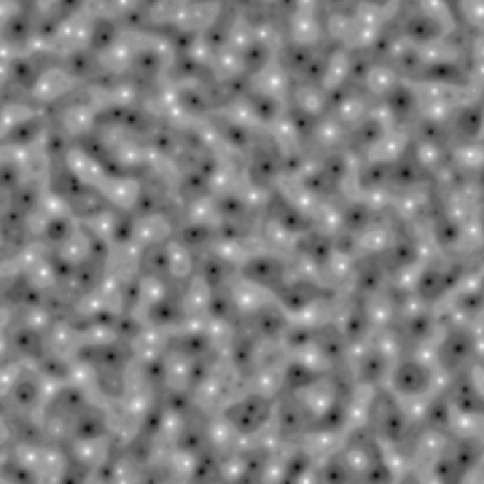
FIG. 3.: Grayscale plot of the stream function $\psi$ at time $t=10^{-2}$. The characteristic scale of vortices $\ell_{E}\sim L/10$ corresponds to the peak of the energy spectrum in Figure 1.

A more significant difference with respect to Navier–Stokes inverse cascade is the presence of strong vortices, as shown in Figure 3. Vortices in CHM turbulence are injected at the forcing scale and they organize themselves to form a random pattern on the characteristic scale $\ell_{E}$. This dynamical scale is associated to the peak of the spectrum of Figure 1. Vortex dynamics slows down as $\ell_{E}$ increases as $\tau(\ell_{E})\sim\ell_{E}^{8/3}$. Thus, in the limit of large Reynolds number the system will end in a disordered pattern of quenched vortices forming a kind of “turbulent glass”.

An important consequence of the presence of strong vortices is that the statistics of the velocity field strongly deviates from Gaussianity. In Figure 4 we plot the pdf of longitudinal and transverse velocity differences at three different scales within the inertial range. The effect of vortices is evident by the presence of large “wings” in the tails, in particular on the transverse velocity differences which are more sensible to a rotating structure.

In conclusion, we have shown that Kolmogorov “3/2” law for two-dimensional energy cascade in Charney-Hasegawa-Mima turbulence is independent on the value of the intrinsic scale $\lambda$. Velocity statistics satisfies Kolmogorov scaling with non-universal coefficients. In the asymptotic limit $\lambda\to\infty$ the Kolmogorov constant is found to be about $2$ times the Navier–Stokes case [10]. Strong coherent vortices are found to emerge at the forcing scale and aggregate to form a pattern of quenched vortices at large scale. As a consequence of the presence of vortices, strong deviations from Gaussianity are observed in the velocity field.

FIG. 4.: Probability density functions of longitudinal (a) and transverse (b) velocity differences at separations $\ell=0.05$ ($+$), $\ell=0.1$ ($\times$) and $\ell=0.2$ ($*$) at time $t=10^{-2}$. Dashed line represents Gaussian distribution.

- [1] R.H. Kraichnan, Phys. Fluids, 10, 1417, (1967).
- [2] G. Boffetta, A. Celani and M. Vergassola, Phys. Rev. E 61, R29 (2000)
- [3] J. McWilliams, J. Fluid Mech. 146, 21 (1984).
- [4] L.M. Smith and V. Yakhot, Phys. Rev. Lett. 71, 352 (1993).
- [5] J.C. Charney, J. Atmos. Sciences 28 1087 (1971).
- [6] A. Hasegawa and K. Mima, Phys. Fluids 21 87 (1978).
- [7] R. Salmon R., Geophysical Fluid Dynamics (Oxford University Press, New York, 1998).
- [8] N. Kukharkin, S.A. Orszag and V. Yakhot, Phys. Rev. Lett. 75, 2486 (1995).
- [9] V.D. Larichev V.D. and J.C. McWilliams J.C., Phys. Fluids A 3, 938 (1991).
- [10] M. Ottaviani and J.A. Krommers, Phys. Rev. Lett. 69, 2923 (1992).
- [11] D. Fyfe and D. Montgomery, Phys. Fluids 22, 246 (1979).
- [12] T. Watanabe, H. Fujisaka and T. Iwayama, Phys. Rev. E 55, 5575 (1997).
- [13] U. Frisch, Turbulence. The legacy of A.N. Kolmogorov (Cambridge University Press, Cambridge, 1995).
- [14] V. Yakhot, Phys. Rev. E 60, 5544 (1999).