Angular momentum localization in oval billiards

Abstract

Angular momentum ceases to be the preferred basis for identifying dynamical localization in an oval billiard at large excentricity. We give reasons for this, and comment on the classical phase-space structure that is encoded in the wave functions of “leaky” dielectric resonators with oval cross section.

PACS: 05.45.Mt, 42.15.-i, 42.25.-p

Geometric optics is an important engineering tool because of its explanatory and predictive power, even when wave effects are present, as is the case in resonant cavities. Nevertheless, quantum chaos has not been widely recognized as an issue in optical resonators until recently [1], because the engineer often has the freedom to choose geometries for which either the ray picture is simple or the wave equation is separable (up to small perturbations). This is a luxury that we do not usually have in naturally occuring, “self-assembled” optical resonators such as, e.g., aerosol droplets [2, 3] or microcrystallites [4].; these examples typically have mixed phase spaces. What we learn from such systems in turn allows us to accept chaotic ray dynamics as a way to introduce added freedom into the design of optical devices in a wide range of material systems, such as semiconductor microdisks [5, 6], polymers and glasses [7, 8, 9]. One of the essential phenomena that makes chaotic resonators useful in this respect is dynamical localization, because it allows cavity resonances with decay rates that exceed the values expected from classical ray considerations. Mixed dynamics does not necessarily make it impossible to identify localization [10], provided the classical phase space stucture is properly taken into account. In this paper, we discuss how localization can be characterized in oval dielectric cavities.

From the quantum-chaos perspective, dielectric microcavities allow us to study the ray-wave duality in a class of open billiard systems bounded by “penetrable” walls which introduce an escape condition in phase space [11]. This openness arises because the internal and external region are coupled across the dielectric-air interface. In many cases this interface can be considred as abrupt on the scale of the wavelength, in which case one arrives at a set of polarization-dependent dielectric boundary conditions which in the ray limit correspond to Fresnel’s laws of reflection. The latter have two basic consequences: (a) if the cavity has refractive index $n$ and the outside is assumed to be air, then rays hitting the surface with angle of incidence greater than $\chi_{c}\equiv\arcsin 1/n$, measured with respect to the normal, undergo total internal reflection. (b) the interface exhibits a finite reflectivity even at normal incidence, $\chi=0$, given by $R=(n-1)^{2}/(n+1)^{2}$; this “ray splitting” implies that rays violating the total-internal-reflection condition may still continue along an internal trajectory with attenuated amplitude [12]. In fact, for large refractive index $n$, the limit of a closed cavity with reflectivity $R=1$ is approached.

In the quantum-classical transition under such circumstances, the competition between the internal time scales (as set most prominently by the density of levels) and the state-dependent decay rates must be taken into account [13, 14, 15]. This becomes especially interesting in cavities with mixed phase spaces because of their intricate temporal evolution [16, 17]. The main objects of study in microlaser design are single, isolated resonances. The reason is that the properties of a laser are typically determined by the spatial and emission characteristics of only one or a few quasibound states. In a single-mode laser, it is the state whose $k$ lies closest to the real axis [18]. In contrast to the random-wave assumption that is justified in the presence of hard chaos [19], highly anisotropic intensity patterns of wave functions are typical for mixed systems. These are in fact desirable in a laser because anisotropy can translate to focused emission[20]. Individual quasibound states can be studied in great detail in microlaser experiments, because one can make spatially and spectrally resolved images of the emitter under various observation angles [3].

The numerical aspects of the electromagnetic scattering problem are challenging and have several decades of history, particularly in atmospheric sciences. If the dielectric constant can be assumed piecewise constant in the spatial domains defining the scatterer, one computational method is that of wavefunction matching: in each dielectric region, a “Treftz basis” is introduced [21], consisting of free-space stationary solutions at a fixed wavenumber $k$. The unknown expansion coefficients of a true wave solution in this basis are determined by imposing the dielectric boundary conditions. In the present study, we are interested in quasibound states of a cylindrical dielectric surrounded by air. For simplicity, we specialize to the case where the electric field is polarized parallel to the cylinder axis, so that Maxwell’s equations reduce to a scalar wave equation [22]. The internal and external wave functions

$$\psi_{\rm int}(r,\phi) = \sum\limits_{m}A_{m}\,J_{m}(nkr)\,e^{im\,\phi},$$ (1)

$$\psi_{\rm ext}(r,\phi) = \sum\limits_{m}B_{m}\,H_{m}^{(1)}(kr)\,e^{im\,\phi}.$$ (2)

satisfy the usual quantum mechanical boundary conditions at the interface,

$$\psi_{\rm int}=\psi_{\rm ext}\quad{\rm and}\quad\partial\psi_{\rm int}/\partial{\bf e}=\partial\psi_{\rm ext}/\partial{\bf e}.$$ (3)

Here, $r$ and $\phi$ are polar coordinates, ${\bf e}$ the outward normal; $k$ is the free-space wavenumber, and $m$ labels angular momentum. Implicit in the form of $\psi_{\rm ext}$ is the condition that only outgoing cylindrical waves be present in the exterior, i.e. the solutions will represent emission without any incoming wave [26] – appropriate for fluorescence or lasing. The resulting homogenous system of Eq. (3) for the $A_{m}$, $B_{m}$ has a nontrivial solution only at a set of discrete, complex values of $k$.

One advantage of Eq. (1) is that it permits a reformulation in terms of the internal scattering matrix of the 2D cross-sectional billiard, in the sense of the “scattering approach to quantization” [23]. However, it is by no means clear that these expansions in angular momentum eigenfunctions with coefficients $A_{m}$, $B_{m}$ converge. The assumption that this is in fact the case is known as the Rayleigh hypothesis [24, 25]. For definiteness, the convex boundaries which shall serve as our model systems are parametrized in polar coordinates by two-dimensional multipoles of constant area,

$$r(\phi)=R\,\left(1+\epsilon\cos(\nu\phi)\right)/\sqrt{1+\epsilon^{2}/2},$$ (4)

where $\nu=1,\,2\ldots$ and $\epsilon$ measures the fractional deformation. The simplest cases are the Limacon shape ($\nu=1$) and the quadrupole ($\nu=2$). Convergence problems arise if the cross section is too strongly deformed, so that the radii of convergence of the inner or outer expansion, Eqs. (1) and (2) intersect the boundary; this can make it impossible to formulate the matching conditions.

As long as the shape is convex, however, numerical experience shows [26] that the problem can be regularized over a wide range of deformations by performing the wavefunction matching at a discrete number $N$ of points in real space and making the number $M$ of angular momenta $m$ in Eq. (1) smaller than $N$. The resulting rectangular matrix problem can then be solved by singular-value decomposition [27]. Additional improvment can be achieved by finding two or more choices of origin for the polar coordinates such that the respective domains of convergence for all resulting versions of Eq. (1), taken together, cover the boundary completely. The additional unknowns in these expansions are then connected by analytical continuation. A simple example for this analytical-continuation approach is the annular billiard [28, 29], in which a circle with an eccentric circular inclusion permits expansions of the type Eq. (1), centered either at the inner or outer circle; the connection between the two expansions is given analytically via the addition theorems for Bessel functions.

There are no truly bound states in this finite-sized 2D photonic system; the same is true for the generalization to a three-dimensionally confined cavity of finite extent. This is the reason for having to permit complex $k$ above, assuming $n$ is real. The fact that all states are metastable distinguishes these systems from the otherwise similar subject of attractive wells in quantum mechanics. This is a reminder of the inequivalence between optical and quantum-mechanical wave equations. Microwave experiments [30, 31, 32] can under certain restrictions emulate of Schrödinger’s equation, if the genuinely electrodynamic aspects of the resonator (resulting from the vectorial nature and hyperbolic charactistics of Maxwell’s time-dependent wave equations) are not important. In dielectric optical cavities, on the other hand, one is often forced by the intended applications to go beyond this analogy [33].

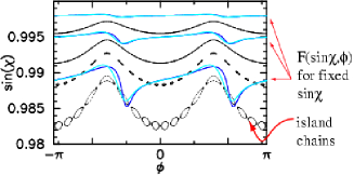
Figure 1: A narrow strip of the Poincaré section for a quadrupole with $\epsilon=0.1$, magnifying the whispering-gallery region. Superimposed on the high-order island chains and invariant KAM curves are plots of the kick strength functions.

As was first argued in Ref. [20], the Poincaré map of the billiard, Eq. (4), contains the essential information determining the emission characteristics of the corresponding resonator. Therefore, it is necessaery to understand the properties of this map in detail. It can be written in the form

$$\sin{\bar{\chi}} = \sin\chi+F({\bar{s}},\sin\chi),$$ (5)

$${\bar{s}} = s+G(s,\sin\chi),$$ (6)

where $s$ is the arc length along the boundary and the bar denotes the new coordinates after one iteration of the map. The functions $F$ and $G$ contain the nonlinearity of the dynamics, as shown in Fig. 1 where we plot $F$ versus final position $s$ for three fixed values of $\sin\chi$. Note that the amplitude of the nonlinearity goes to zero as $\sin\chi\to 1$. To quantify this, Fig. 2 plots the root-mean-square of $F$ versus starting $\sin\chi$. A fit with $(1-\sin^{2}\chi)^{3/2}$ shows good agreement. The reason for this functional form with its non-analyticity at $\sin\chi=1$ is understandable from very general considerations:

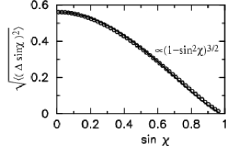
Figure 2: RMS deviation of $\sin\chi$ from its initial value for one iteration of the billiard map for the quadrupole at $\epsilon=0.08$, averaged over final position ${\bar{s}}$. Circles are from the exact ray dynamics, solid line is a fit with $(1-\sin^{2}\chi)^{3/2}$.

If one considers $F$ as a function of $\cos\chi$ instead of $\sin\chi$, then a Taylor expansion around $\cos\chi=0$ yields a mapping equation of the form

$$\cos{\bar{\chi}}\approx f_{0}({\bar{s}})+f_{1}({\bar{s}})\,\cos\chi+f_{2}({\bar{s}})\,\cos^{2}\chi+\ldots$$ (7)

We expect $f_{0}\equiv 0$ since a trajectory starting with $\cos\chi=0$ must end up with $\cos{\bar{\chi}}=0$ (corresponding to “rolling” or “grazing” motion along the convex surface. Using this expansion for $\sin\chi\to 1$ in Eq. (5), we obtain

$$\sin{\bar{\chi}}\approx\sin\chi-f_{1}({\bar{s}})\,f_{2}({\bar{s}})\,(1-\sin^{2}\chi)^{3/2}.$$ (8)

The resulting $\sin\chi$ - dependence in Fig. 2 suggests that the map of the convex billiard should exhibit invariant curves in the “whispering-gallery” (WG) region ($\sin\chi\to 1$) at arbitrarily large deformations, where other KAM curves (such as the one belonging to the inverse golden mean winding number) have been broken up.

The last statement is in fact implied by Lazutkin’s theorem [34], which however requires 553 continuous derivatives of $r(\phi)$ to prove that invariant WG tori exist with nonzero Lebesgue measure. Here, we can go beyond the mere existence statement and ask what consequences the existence of a stable WG region has for the neighboring phase space. We shall find that only a much smaller number of 3 continuous derivatives enters the physical considerations describing the phaes space of the convex billiard. We base our argument on an adiabatic approximation used in Ref. [35], which will be discussed further below. There, the unknown multiplier $f_{1}({\bar{s}})\,f_{2}({\bar{s}})$ of Eq. (8) is determined from geometric considerations to yield

$$\sin{\bar{\chi}}=\sin\chi-\frac{2\kappa^{\prime}({\bar{s}})}{3\kappa^{2}({\bar{s}})}\,(1-\sin^{2}\chi)^{3/2},$$ (9)

where $\kappa(s)$ is the curvature and $\kappa^{\prime}$ its derivative. In Ref. [35], this together with a similar approximation for the position mapping function $G({\bar{s}},\sin\chi)$ is used to convert the amplitudes of the two mapping equations, Eq. (5) and Eq. (6), into a differential equation:

$$\frac{d\sin\chi}{ds}\approx\frac{\sin{\bar{\chi}}-\sin\chi}{{\bar{s}}-s}=\frac{F({\bar{s}},\sin\chi)}{G({\bar{s}},\sin\chi)}\approx\frac{F(s,\sin\chi)}{G({s,\sin\chi)}},$$ (10)

which can be solved by separation of variables to obtain an adiabatic invariant curve

$$p(s)\approx\sqrt{1-\left(1-\sigma^{2}\right)\,\kappa^{3/2}(s)}.$$ (11)

Here, we use the abbreviation

$$p\equiv\sin\chi,$$ (12)

which is the momentum conjugate to $s$. The intergation constant $\sigma$ parametrizes the value around which $p(s)=\sin\chi(s)$ oscillates.

The range of validity of Eq. (9) extends beyond the WG limit $\sin\chi\approx 1$, as Fig. 2 already suggests. A position mapping equation which also yields reasonable agreement for the whole range of possible initial $\sin\chi$ has been derived in Ref. [26] by introducing a generating function $Z({\bar{s}},p)$ for the billiard map. From $Z$, the new momentum and old positions are obtained as partial derivatives,

$${\bar{p}}=\left.\frac{\partial Z}{\partial{\bar{s}}}\right|_{p},\qquad s=\left.\frac{\partial Z}{\partial p}\right|_{\bar{s}}.$$ (13)

This definition guarantees that the map is area preserving. The first equation above is just what we already obtained in Eq. (9), so we can infer $Z({\bar{s}},p)$ by integrating Eq.  (9) over ${\bar{s}}$. This leads to

$$Z({\bar{s}},p)=p\,{\bar{s}}+\frac{2}{3\kappa({\bar{s}})}\,(1-p^{2})^{3/2}+c(p),$$ (14)

where $c(p)$ is the integration constant which may still depend on $p$. Applying the second of Eqs. (13) to this result, we arrive at the position mapping equation,

$$s={\bar{s}}+c^{\prime}(p)-\frac{2p}{\kappa({\bar{s}})}\,(1-p^{2})^{1/2}.$$ (15)

This can in principle be inverted to get ${\bar{s}}$ as a function of $p$ and $s$. We dispose of the arbitrary $c^{\prime}(p)$ in such a way that Eq. (15) reduces to the exact expression in the circular billiard where $\kappa\equiv 1$. The result is, reinstating $\sin\chi$ for $p$,

$$s={\bar{s}}-2\,\arccos(\sin\chi)+2\,(1-\frac{1}{\kappa({\bar{s}})})\,\sin\chi\,(1-\sin^{2}\chi)^{1/2}.$$ (16)

In contrast to the analogous result in Ref. [35], this position map remains well-defined over the whole range of $|\sin\chi|=0\ldots 1$. The billiard shape enters in Eqs. (9) and (16) only through the curvature as a function of ${\bar{s}}$.

The “effective map” as defined through Eqs. (9) and (16) reproduces the global structure as well as local detail of the true Poincaré sections for the Limacon and quadrupole billiards [26]. Although some additional rescaling of the deformation parameter $\epsilon$ is required for best agreement, one can use the effictive map to understand classical properties of the billiard, such as the existnce of Lazutkin’s invariant tori. The utility of this approach consists in breaking the billiard problem up into two distinct subproblems: the geometric analysis leading to the Poincaré mapping on the one hand, and the nonlinear dynamics of that map on the other hand. We now wish to apply Eqs. (9) and (16) to our understanding of Lazutkin’s theorem.

The adiabatic approximation leading to Eq. (9) relies on the fact that for trajectories in the whispering-gallery region, there is a separation of time scales between slow changes in the average $\sin\chi$ and a fast circulation in arc length $s$ around the boundary; this separation becomes infinitely wide as $\sin\chi\to 1$, as required by Lazutkin’s theorem. In other words, if multiple iterations of the map return ${\bar{s}}$ to an inifintesimal neighborhood $\Delta s$ of its initial value $s$, then the same will automatically be true for the second variable $\sin\chi$, in such a way that the derivative in Eq. (10) exists. Now let us approach the adiabatic limit from the side of a chaotic trajectory described by the effective map, for which that derivative is ill-defined but a finite separation of time scales still exists. Then we can then ask for the local diffusion constant, defined as the proportionality constant between the rms spread of $\sin\chi$ (averaged over ${\bar{s}}$) and the number of mapping iterations $n$,

$$\langle\left(\Delta p(n)\right)^{2}\rangle = D(p_{0})\,n$$

$$D(p_{0}) = \frac{4}{9}\,\frac{1}{2\pi}\,(1-p_{0}^{2})^{3}\,\int\limits_{0}^{L}\left[\frac{{\dot{\kappa}}(s)}{\kappa^{2}(s)}\right]^{2}\,ds,$$ (17)

where $L$ is the circumference of the boundary. The assumption of a diffusive growth in the variance of $\sin\chi$ leads us to make the random phase approximation [36] for $s$, as contained in the integral over $s$ above.

In fact, this approximation is hard to justify in generic billiards with a mixed phase space, but improvements can in principle be made by including an average over a finite number of mapping steps in the definition of $D$. The main conclusion from Eq. (17) is that the diffusion constant follows the $\sin\chi$ dependence of Fig. 2 (squared) and hence vanishes for $\sin\chi\to 1$. Now define the (discrete) diffusion time in $p$, $\tau_{p}$ to be the number of iterations it takes to diffuse across the whole allowed $p$-interval; define further the phase randomization time $\tau_{s}$ as the number of reflections necessary before $s$ has wrapped once around the boundary. Then from Eq. (17),

$$\tau_{p}\propto\frac{1}{(1-p^{2})^{3}},$$ (18)

and from Eq. (16),

$$\tau_{s}\propto\frac{1}{p\,\sqrt{1-p^{2}}}.$$ (19)

The proportionality constants are functions of the deformation alone. As the whispering-gallery limit is approached, $\tau_{p}$ diverges much faster than $\tau_{s}$, so that the existence of invariant curves can be inferred as $\sin\chi\to 1$. Since no more than the first derivative of $\kappa$ appears in the “kick strength” of the analytic mapping of Eqs. (9) and (16), this suggests that only three continuous derivatives of the boundary suffice to explain Lazutkin’s tori.

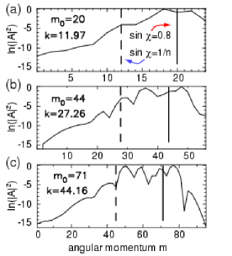
Figure 3: Decadic logarithm of the angular momentum coefficients $|A_{m}|^{2}$ in Eq. (1) for three differnt quasibound states of the dielectric quadrupole with $n=2$ and $\epsilon=0.08$; all states are semiclassically quantized at approximately the same value of the adiabatic constant $\sigma$, at wavenumbers $kR\approx 11.97,\,27.26,$ and $44.16$.

As an example of how the above remarks on phase space transport properties in a convex billiard help us understand the quasibound states of the corresponding resonator, Fig. 3 shows how dynamical localization can be discerned in the numerical solutions of the wave problem. The same states displayed here have been investigated in Ref. [37] as a function of the deformation $\epsilon$. There, an adiabatic quantization based on the invariant curves Eq. (11) was introduced, according to which all three states were found to correspond to approximately the same value of $\sigma$, i.e. the adiabatic invariant characterizing the phase-space location of the state. The wavenumbers $k$ of the lowest and highest state in Fig. 3 differ by roughly a factor of four, and as a consequence the decay rates in the limit of a circular resonator range over approximately ten orders of magnitude. However, at large deformation $\epsilon$ where the escape from the resonator is dominated by classical ray diffusion, the resonance widths $\delta k$ are found to be nearly wavelength independent. As a correction to this classical behavior, one observes a tendency toward slightly faster decay at larger wavenumber $k$. This correction, together with the fact that the adiabatic quantization for the resonance positions actually agreed better with the exact results at smaller $k$ led to the hypothesis [37] that dynamical localization is present in the states under consideration, especially at low $k$.

Figure 3 allows us to identify qualitatively the effect of dynamical localization in a mixed phase space with open boundary conditions. The solid vertical lines in the figure indicate the semiclassically expected maxima of the angular momentum distribution for the three wavefunctions. This semiclassical quantization is performed by applying the EBK method to the invariant curves of Eq. (11). The quantized values of $\sigma$ are then translated back to angular momentum by using the approximate semiclassical relation known from the circle,

$$m=n\,kR\,\sin\chi.$$ (20)

We use this together with our classical considerations to estimate the spread in $m$ that is evident in the wavefunctions.

The interval of $m$ on the horizontal axis corresponds to the range $0\leq\sin\chi\leq 1$; the dashed vertical lines indicate the “ionization border” $\sin\chi=1/n$. At $\epsilon=0.08$ in the quadrupole, unbroken KAM curves exist only above $\sin\chi\approx 0.9$. The sharp falloff in $|A_{m}|$ at large $m$ is due to the classical inaccessibility of the high-$\sin\chi$ region by diffusion – it directly shows the imbalance in the nonlinearity between large and small $\sin\chi$.

Exponential localization is identifiable in Fig. 3 only to the left of a plateau surrounding the semiclassical maxima, of width $\Delta m\approx 4$ in (a) and $\Delta m\approx 10$ in (b). The explanation for this is that the adiabatic curve, Eq. (11), for $\sigma=0.8$ oscillates between $\sin\chi_{max}\equiv=0.89$ and $\sin\chi_{min}=0.72$. The latter translates to an angular momentum spread of $\Delta m\approx 4,\,9,\,$ and $14$, respectively, for the states quantized at $kR\approx 11.97,\,27.26,$ and $44.16$. The agreement with the Figure confirms that the semiclassical maximum, ionization border and width of the plateau in $m$ all scale proportional to $kR$. This leaves us with an $m$ interval $\delta m$ to the right of the escape threshold, of width $\delta m\approx n\,kR\,(\sin\chi_{min}-\sin\chi_{c})=n\,kR\,(0.72-0.5)$, corresponding to a classically diffusive region in which a probability decay should be observed. In the Figure, an exponential decrease away from the semiclassical plateau is discernible for $kR=11.97$ (a) and $27.26$ (b), whereas the state at $kR=44.16$ (c) exhibits large angular momentum components over the whole classically confined region. The localization lengths $\xi$ estimated from the observed slopes for the two lower-$kR$ states are approximately in a ratio of $2\,:\,1$, in reasonable agreement with the factor of two between the respective wavelengths. This is the expected behavior [38], because the diffusion constant entering $\xi$ is the same in all resonances.

Angular momentum as a prefered basis for measuring dynamical localization is a useful initial choice in the oval billiard, but as the existence of the plataeus above indicates, it is not strictly the correct one. Recall that $\sigma$, and not $\sin\chi$ or angular momentum, is the adiabatic invariant in the semiclassical quantization for the states in Fig. 3. This can be made very clear by comparing to the special case of the ellipse where the adiabatic curve Eq. (11) becomes exact. Then $\sigma$, which in the circle is the angular momentum, acts as a constant of the motion while $\sin\chi$ still oscillates. Clearly, there is no diffusion although the angular momentum decomposition shows a spread $\Delta m$ whose width is determined by the eccentricity. For the oval billiard, this means that $\sigma$ should be considered as the diffusing variable. Classically, the transformation from $\sin\chi$ to $\sigma$ is given by Eq. (11). Wave-mechanically, the goal will be to project the true wave function $\psi$ onto a Treftz basis defined by these adiabatic invariant curves.

Judging by the results presented here, this is a worthwile program for future work because a better-adapted basis significantly expands the interval over which one is allowed to assume the separation of time scales which leads to classical diffusion in the first place. In billiards that remain close to a circle, such as a short stadium [38] or rough billiard [39, 40] this problem does not arise. However, in oval billiards, these classical considerations apply. Moreover, the breakdown of the Rayleigh hypothesis makes it not only desirable but necessary to abandon angular momentum as the basis in which to detect dynamical localization.

I would like to thank Steve Tomsovic for valuable discussions.

References

- [1] Stone, A. D., contribution in this issue
- [2] Mekis, A. et al. Phys. Rev. Lett.75, 2682 (1995).
- [3] Chang, S. et al., submitted to J. Opt. Soc. Am. B (2000)
- [4] Vietze, U. et al., Phys. Rev. Lett. 81, 4628 (1998)
- [5] Yamamoto, Y. and Slusher, R. E., Physics Today 46, 66 (1993)
- [6] Zhang, J. P. et al., Phys. Rev. Lett. 75, 2678 (1995)
- [7] Dodabalpur, A. et al., Science 277, 1787 (1997)
- [8] Collot, L., Lefevre-Seguin, V., Raimond, M. and Haroche, S., Europhys. Lett. 23, 327 (1993)
- [9] Serpengüzel, A., Arnold, S. and Griffel, G., Opt. Lett. 20, 654 (1995)
- [10] Robinson, J. C. et al., Phys. Rev. Lett. 75, 3963 (1995)
- [11] Borgonovi, F., Guarneri, I. and Shepelyansky, D. L., Phys. Rev. A 43, 4517 (1991)
- [12] Kohler, A. and Blümel, R., Ann. Phys. New York 267, 249 (1998)
- [13] Prigogine, I., Phys. Rep. 219, 93 (1992)
- [14] Kohler, S. et al., Phys. Rev. E 58, 7219 (1998)
- [15] Braun, D., Braun, P. L. and Haake, F., Physica D 131, 265 (1999)
- [16] Zaslavsky, G. M., Physics Today 52, 39 (1999)
- [17] Huckestein, B., Ketzmerick, R. and Lewenkopf, C. H., Phys. Rev. Lett. 84, 5504 (2000)
- [18] Misirpashaev, T. Sh., Beenakker, C.W.J., Phys. Rev. A 57, 2041 (1998)
- [19] Eckhardt, B., Dörr, U., Kuhl, U. and Stöckmann, H.-J., Europhys. Lett. 46, 134 (1999)
- [20] Nöckel, J. U., Stone, A. D. and Chang, R. K., Optics Letters 19, 1693 (1994);
- [21] Petrov, P. K. and Babenko, V. A., J. Quant. Spectroscop. Rad. Trans. 63, 237 (1999)
- [22] Nöckel, J. U. and Stone, A. D., in: “ Optical Processes in Microcavities”, edited by R. K. Chang and A. J. Campillo (World Scientific, Singapore, 1996)
- [23] Smilanski, U., in: Proc. 1994 Les Houches Summer School LXI on Mesoscopic Quantum Physics, edited by E. Akkermans, G. Montambaux, J. L. Pichard and J.Zinn-Justin, p. 373 (Elsevier, Amsterdam 1995)
- [24] van den Berg, P. M. and Fokkema, J. T., IEEE Trans. Anten. Propag. AP-27, 577 (1979)
- [25] Barton, J. P., Appl. Opt. 36, 1312 (1997)
- [26] Nöckel, J. U., Dissertation Thesis, Yale University (1997)
- [27] Penrose, R., Proc. Cambridge Phil. Soc., no. 52 (1956)
- [28] Doron, E. and Frischat, S., Phys. Rev. Lett. 75, 3661 (1995)
- [29] Hackenbroich, G. and Nöckel, J. U., Europhys. Lett. 39, 371 (1997)
- [30] Stein, J. and Stöckmann, H.-J., Phys. Rev. Lett. 68, 2867 (1992)
- [31] Alt, H. et el., Phys. Rev. E 54, 2303 (1996)
- [32] Sridhar, S. and Heller, E., Phys. Rev. A 42, R1728 (1992)
- [33] Hentschel, M. and Nöckel, J. U. (to be published in Proceedings of the Royal Netherlands Academy of Arts and Sciences, 2000
- [34] Lazutkin, V. F., “ KAM Theory and Semiclassical Approximations to Eigenfunctions”, (Springer, New York,1993)
- [35] M. Robnik and Berry, M. V., J. Phys. A: Math. Gen. 18, 1361 (1985)
- [36] Lichtenberg, A. J. and Lieberman, M. A., Physica D 33, 211 (1988)
- [37] Nöckel, J. U. and Stone, A. D., Nature 385, 45 (1997)
- [38] Borgonovi, F., Casati, G. and Li, B., Phys. Rev. Lett. 77, 4744 (1996)
- [39] Frahm, K. and Shepelyansky, D. L., Phys. Rev. Lett. 79, 1833 (1997)
- [40] Starykh, O. A. et al., cont-mat/0001017