From Coupled Dynamical Systems to Biological Irreversibility

Abstract

In the first half of the paper, some recent advances in coupled dynamical systems, in particular, a globally coupled map are surveyed. First, dominance of Milnor attractors in partially ordered phase is demonstrated. Second, chaotic itinerancy in high-dimensional dynamical systems is briefly reviewed, with discussion on a possible connection with a Milnor attractor network. Third, infinite-dimensional collective dynamics is studied, in the thermodynamic limit of the globally coupled map, where bifurcation to lower-dimensional attractors by the addition of noise is briefly reviewed.

Following the study of coupled dynamical systems, a scenario for developmental process of cell society is proposed, based on numerical studies of a system with interacting units with internal dynamics and reproduction. Differentiation of cell types is found as a natural consequence of such a system. “Stem cells” that either proliferate or differentiate to different types generally appear in the system, where irreversible loss of multipotency is demonstrated. Robustness of the developmental process against microscopic and macroscopic perturbations is found and explained, while irreversibility in developmental process is analyzed in terms of the gain of stability, loss of diversity and chaotic instability. Construction of a phenomenology theory for development is discussed in comparison with the thermodynamics.

1 Introduction

How should we understand the origin of biological irreversibility?

As an empirical fact, we know that the direction from the alive to the dead is irreversible. At a more specific level, we know that, in a multicellular-organism with a developmental process, there is a definite temporal flow; Through the developmental process, the multipotency, i.e., the ability to create a different type of cells, decreases. Initially, the embryonic stem cell has totipotency, and has the potentiality to create all types of cells in the organism. Then a stem cell can create a limited variety of cells, having multipotency. This hierarchical loss of multipotency terminates at a determined cell, which can only replicate its own type, in the normal developmental process. The degree of determination increases in the normal course of development. How can one understand such irreversibility?

Of course this question is not easy to answer. However, it should be pointed that

1) It is very difficult to imagine that this irreversibility is caused by a set of specific genes. The present irreversibility is too universal to be attributed to characteristics of a few molecules.

2) It is also impossible to simply attribute this irreversibility to the second law of thermodynamics. One can hardly imagine that the entropy, even if it were possible to be defined, suddenly increases at the death, or successively increases at the cell differentiation process. Furthermore, it should be generally very difficult to define a thermodynamic entropy to a highly nonequilibrium system such as a cell.

Then what strategy should we choose?

A biological system contains always sufficient degrees of freedom, say, a set of chemical concentrations in a cell, which change in time. Then, one promising strategy for the study of a biological system lies in the use of dynamical systems[1]. By setting a class of dynamical systems, we search for universal characteristics that are robust against microscopic and macroscopic fluctuations.

A biological unit, such as a cell, has always some internal structure that can change in time. As a simple representation, the unit can be represented by a dynamical system. For example, consider a representation of a cell by a set of chemical concentrations. A cell, however, is not separated from the outside world completely. For example, isolation by a biomembrane is flexible and incomplete. In this way, the units, represented by dynamical systems, interact with each other through the external environment. Hence, we need a model consisting of the interplay between inter-unit and intra-unit dynamics. For example, the complex chemical reaction dynamics in each unit (cell) is affected by the interaction with other cells, which provides an interesting example of “intra-inter dynamics”. In the ‘intra-inter dynamics’, elements having internal dynamics interact with each other. This type of intra-inter dynamics is not necessarily represented only by the perturbation of the internal dynamics by the interaction with other units, nor is it merely a perturbation of the interaction by adding some internal dynamics.

As a specific example of the scheme of intra-inter dynamics, we will mainly discuss the developmental process of a cell society accompanied by cell differentiation. Here, the intra-inter dynamics consists of several biochemical reaction processes. The cells interact through the diffusion of chemicals or their active signal transmission.

If $N$ cells with $k$ degrees of freedom exist, the total dynamics is represented by an $Nk$-dimensional dynamical system (in addition to the degrees of freedom of the environment). Furthermore, the number of cells is not fixed in time, but they are born by division (and die) in time.

After the division of a cell, if two cells remained identical, another set of variables would not be necessary. If the dynamical system for chemical state of a cell has orbital instability (such as chaos), however, the orbits of chemical dynamics of the (two) daughters will diverge. Hence, the number of degrees of freedom, $Nk$, changes in time. This increase in the number of variables is tightly connected with the internal dynamics. It should also be noted that in the developmental process, in general, the initial condition of the cell states is chosen so that their reproduction continues. Thus, a suitable initial condition for the internal degrees of freedom is selected through interaction.

Now, to study a biological system in terms of dynamical systems theory, it is first necessary to understand the behavior of a system with internal degrees of freedom and interaction[4], This is the main reason why I started a model called Coupled Map Lattice [5] (and later Globally Coupled Map[6]) about 18 years ago. Indeed, several discoveries in GCM seem to be relevant to understand some basic features in a biological system. GCM has provided us some novel concepts for non-trivial dynamics between microscopic and macroscopic levels, while the dynamic complementarity between a part and the whole is important to study biological organization[7]. In the present paper, we briefly review the behaviors of GCM in §2, and discuss some recent advances in §3 - §5, about dominance of Milnor attractors, chaotic itinerancy, and collective dynamics. Then we will switch to the topic of development and differentiation in an interacting cell system. After presenting our model based on dynamical systems in §6, we give a basic scenario discovered in the model, and interpret cell differentiation in terms of dynamical systems. Then, the origin of biological irreversibility is discussed in §9. Discussion towards the construction of phenomenology theory of development is given in §10.

2 High-dimensional chaos revisited

The simplest case of global interaction is studied as the “globally coupled map” (GCM) of chaotic elements [6]. A standard example is given by

$$x_{n+1}(i)=(1-\epsilon)f(x_{n}(i))+\frac{\epsilon}{N}\sum_{j=1}^{N}f(x_{n}(j))$$ (1)

where $n$ is a discrete time step and $i$ is the index of an element ($i=1,2,\cdots,N$ = system size), and $f(x)=1-ax^{2}$. The model is just a mean-field-theory-type extension of coupled map lattices (CML)[5].

Through the interaction, elements are tended to oscillate synchronously, while chaotic instability leads to destruction of the coherence. When the former tendency wins, all elements oscillate coherently, while elements are completely desynchronized in the limit of strong chaotic instability. Between these cases, elements split into clusters in which they oscillate coherently. Here a cluster is defined as a set of elements in which $x(i)=x(j)$ [6]. Attractors in GCM are classified by the number of synchronized clusters $k$ and the number of elements for each cluster $N_{i}$. Each attractor is coded by the clustering condition $[k,(N_{1},N_{2},\cdots,N_{k})]$. Stability of each clustered state is analyzed by introducing the split exponent [6, 9].

An interesting possibility in the clustering is that it provides a source for diversity. In clustering it should be noted that identical chaotic elements differentiate spontaneously into different groups: Even if a system consists of identical elements, they split into groups with different phases of oscillations. Hence a network of chaotic elements gives a theoretical basis for isologous diversification and provides a mechanism for the origin of diversity and complexity in biological networks [11, 10].

In a globally coupled chaotic system in general, the following phases appear successively with the increase of nonlinearity in the system ($a$ in the above logistic map case) [6]:

(i) Coherent phase: Only a coherent attractor ($k=1$) exists.

(ii) Ordered phase: All attractors consist of few ($k=o(N)$) clusters.

(iii) Partially ordered phase: Attractors with a variety of clusterings coexist, while most of them have many clusters ($k=O(N)$).

(iv) Turbulent phase: Elements are completely desynchronized, and all attractors have $N$ clusters.

The above clustering behaviors have universally been confirmed in a variety of systems.

In the partially ordered (PO) phase, there are a variety of attractors with a different number of clusters, and a different way of partitions $[N_{1},N_{2},\cdots,N_{k}]$. The clustering here is typically inhomogeneous: The partition $[N_{1},N_{2},\cdots,N_{k}]$ is far from equal partition. Often this clustering is hierarchical as for the number of elements, and as for the values. For example, consider the following idealized clustering: First split the system into two equal clusters. Take one of them and split it again into two equal clusters, while leave the other without split. By repeating this process, the partition is given by $[N/2,N/4,N/8,\cdots]$. In this case, the difference of the values of $x_{n}(i)$ is also hierarchical. The difference between the values of $x_{n}(i)$ decreases as the above process of partition is iterated. Although the above partition is too much simplified, such hierarchical structure in partition and in the phase space is typically observed in the PO phase. The partition is organized as an inhomogeneous tree structure, as in the spin glass model [8].

We have also measured the fluctuation of the partitions, using the probability $Y$ that two elements fall on the same cluster. In the PO phase, this $Y$ value fluctuates by initial conditions, and the fluctuation remains finite even if the size goes to infinity [12, 13]. It is noted that such remnant fluctuation of partitions is also seen in spin glass models [8].

3 Chaotic Itinerancy and Milnor attractors

In the Partially ordered (PO) phase, there coexist a variety of attractors depending on the partition[12]. To study the stability of an attractor against perturbation, we introduce the return probability $P(\sigma)$, defined as follows[14]: Take an orbit point $\{x(i)\}$ of an attractor in an $N$-dimensional phase space, and perturb the point to $x(i)+\frac{\sigma}{2}rnd_{i}$, where $rnd_{i}$ is a random number taken from $[-1,1]$, uncorrelated for all elements $i$. Check if this perturbed point returns to the original attractor via the original deterministic dynamics (1). By sampling over random perturbations and the time of the application of perturbation, the return probability $P(\sigma)$ is defined as (# of returns )$/$ (# of perturbation trials). As a simple index for robustness of an attractor, it is useful to define $\sigma_{c}$ as the largest $\sigma$ such that $P(\sigma)=1$. This index measures what we call the strength of an attractor.

The strength $\sigma_{c}$ gives a minimum distance between the orbit of an attractor and its basin boundary. In contrast with our naive expectation from the concept of an attractor, we have often observed ‘attractors’ with $\sigma_{c}=0$, i.e., $P(+0)\equiv\lim_{\delta\rightarrow 0}P(\delta)<1$. If $\sigma_{c}=0$ holds for a given state, it cannot be an “attractor” in the sense with asymptotic stability, since some tiny perturbations kick the orbit out of the “attractor”. The attractors with $\sigma_{c}=0$ are called Milnor attractors[15, 16]. In other words, Milnor attractor is defined as an attractor that is unstable by some perturbations of arbitrarily small size, but globally attracts orbital points. The basin of attraction has a positive Lebesgue measure. (The basin is riddled here [17, 18].) Since it is not asymptotically stable, one might, at first sight, think that it is rather special, and appears only at a critical point like the crisis in the logistic map[15]. To our surprise, the Milnor attractors are rather commonly observed around the PO phase in our GCM. The strength and basin volume of attractors are not necessarily correlated. Attractors with $\sigma_{c}=0$ often have a large basin volume.

Still, one might suspect that such Milnor attractors must be weak against noise. Indeed, by a very weak noise with the amplitude $\sigma$, an orbit at a Milnor attractor is kicked away, and if the orbit is reached to one of attractors with $\sigma_{c}>\sigma$, it never comes back to the Milnor attractor. Rather, an orbit kicked out from a Milnor attractor is often found to stay in the vicinity of it[16]. The orbit comes back to the original Milnor attractor before it is kicked away to other attractors with $\sigma_{c}>\sigma$. Furthermore, by a larger noise, orbits sometimes are more attracted to Milnor attractors. Such attraction is possible, since Milnor attractors here have global attraction in the phase space, in spite of their local instability.

Dominance of Milnor attractors gives us to suspect the computability of our system. Once the digits of two variable $x(i)=x(j)$ agree down to the lowest bit, the values never split again, even though the state with the synchronization of the two elements may be unstable. As long as digital computation is adopted, it is always possible that an orbit is trapped to such unstable state. In this sense a serious problem is cast in numerical computation of GCM in general .

Existence of Milnor attractors may lead us to suspect the correspondence between a (robust) attractor and memory, often adopted in neuroscience (and theoretical cell biology). It should be mentioned that Milnor attractors can provide dynamic memory [19, 4] allowing for interface between outside and inside, external inputs and internal representation.

4 Chaotic Itinerancy

Besides the above static complexity, dynamic complexity is more interesting at the PO phase. Here orbits make itinerancy over ordered states with partial synchronization of elements, via highly chaotic states. This dynamics, called chaotic itinerancy (CI), is a novel universal class in high-dimensional dynamical systems. Our CI consists of a quasi-stationary high-dimensional state, exits to “attractor-ruins” with low effective degrees of freedom, residence therein, and chaotic exits from them. In the CI, an orbit successively itinerates over such “attractor-ruins”, ordered motion with some coherence among elements. The motion at “attractor-ruins” is quasistationary. For example, if the effective degrees of freedom is two, the elements split into two groups, in each of which elements oscillate almost coherently. The system is in the vicinity of a two-clustered state, which, however, is not a stable attractor, but keeps attraction to its vicinity globally within the phase space. After staying at an attractor-ruin, an orbit exits from it due to chaotic instability, and shows a high-dimensional chaotic motion without clear coherence. This high-dimensional state is again quasistationary, although there are some holes connecting to the attractor-ruins from it. Once the orbit is trapped at a hole, it is suddenly attracted to one of attractor ruins, i.e., ordered states with low-dimensional dynamics.

This CI dynamics has independently been found in a model of neural dynamics by Tsuda [19], optical turbulence [20], and in GCM. It provides an example of successive changes of relationships among elements.

Note that the Milnor attractors satisfy the condition of the above ordered states constituting chaotic itinerancy. Some Milnor attractors we have found keep global attraction, which is consistent with the observation that the attraction to ordered states in chaotic itinerancy occurs globally from a high-dimensional chaotic state. Attraction of an orbit to precisely a given attractor requires infinite time, and before the orbit is really settled to a given Milnor attractor, it may be kicked away. When Milnor attractors that lose the stability ($P(0)<1$) keep global attraction, the total dynamics can be constructed as the successive alternations to the attraction to, and escapes from, them. If the attraction to robust attractors from a given Milnor attractor is not possible, the long-term dynamics with the noise strength $\rightarrow+0$ is represented by successive transitions over Milnor attractors. Then the dynamics is represented by transition matrix over among Milnor attractors. This matrix is generally asymmetric: often, there is a connection from a Milnor attractor A to a Milnor attractor B, but not from B to A. The total dynamics is represented by the motion over a network, given by a set of directed graphs over Milnor attractors.

In general, the ‘ordered states’ in CI may not be exactly Milnor attractors but can be weakly destabilized states from Milnor attractors. Still, the attribution of CI to Milnor attractor network dynamics is expected to work as one ideal limit .

As already discussed about the Milnor attractor, computability of the switching over Milnor attractor networks has a serious problem. In each event of switching, which Milnor attractor is visited next after the departure from a Milnor attractor may depend on the precision. In this sense, the order of visits to Milnor attractors in chaotic itinerancy may not be undecidable in a digital computer. In other words, motion at a macroscopic level may not be decidable from a microscopic level. With this respect, it may be interesting to note that there are similar statistical features between (Milnor attractor) dynamics with a riddled basin and undecidable dynamics of a universal Turing-machine[21].

5 Collective Dynamics

If the coupling strength $\epsilon$ is small enough, oscillation of each element has no mutual synchronization. In this turbulent phase, $x(i)$ takes almost random values almost independently, and the number of degrees of freedom is proportional to the number of elements $N$, i,e., the Lyapunov dimension increases in proportion to $N$. there remains some coherence among elements. Even in such case, the macroscopic motion shows some coherent motion distinguishable from noise, and there remains some coherence among elements, even in the limit of $N\rightarrow\infty$. As a macroscopic variable we adopt the mean field,

$$h_{n}={1\over N}\sum_{i=1}^{N}f(x_{n}(i)).$$ (2)

In almost all the parameter values, the mean field motion shows some dynamics that is distinguishable from noise, ranging from torus-like to higher dimensional motion. This motion remains even in the thermodynamic limit[24].

This remnant variation means that the collective dynamics $h_{n}(i)$ keeps some structure. One possibility is that the dynamics is low-dimensional. Indeed in some system with a global coupling, the collective motion is shown to be low-dimensional in the limit of $N\rightarrow\infty$ ( see [25, 26].) In the GCM eq.(1), with the logistic or tent map, low-dimensional motion is not detected generally, although there remains some collective motion in the limit of $N\rightarrow\infty$. The mean field motion in GCM is regarded to be infinite dimensional, even when the torus-like motion is observed [27, 28, 29, 30]. Then it is important to clarify the nature of this mean-field dynamics.

It is not so easy to examine the infinite dimensional dynamics, directly. Instead, Shibata, Chawanya and the author have first made the motion low-dimensional by adding noise, and then studied the limit of noise $\rightarrow 0$. To study this effect of noise, we have simulated the model

$$x_{n+1}(i)=(1-\epsilon)f(x_{n}(i))+\frac{\epsilon}{N}\sum_{j=1}^{N}f(x_{n}(j))+\sigma\eta_{n}^{i},$$ (3)

where $\eta_{n}^{i}$ is a white noise generated by an uncorrelated random number homogeneously distributed over [-1,1].

The addition of noise can destroy the above coherence among elements. In fact, the microscopic external noise leads the variance of the mean field distribution to decrease with $N$ [24, 32]. This result also implies decrease of the mean field fluctuation by external noise.

Behavior of the above equation in the thermodynamic limit $N\rightarrow\infty$ is represented by the evolution of the one-body distribution function $\rho_{n}(x)$ at time step $n$ directly. Since the mean field value

$$h_{n}=\int f(x)\rho_{n}(x)dx$$ (4)

is independent of each element, the evolution of $\rho_{n}(x)$ obeys the Perron-Frobenius equation given by,

$$\rho_{n+1}(x)=\int dy{1\over\sqrt{2\pi}\sigma}e^{-{\left(F_{n}(y)-x\right)^{2}\over 2\sigma^{2}}}\rho_{n}(y),$$ (5)

with

$$F_{n}(x)=(1-\epsilon)f(x)+\epsilon h_{n}.$$ (6)

By analyzing the above Perron-Frobenius equation[31], it is shown that the dimension of the collective motion increases as $log(1/\sigma^{2})$, with $\sigma$ as the noise strength. Hence in the limit of $\sigma\rightarrow 0$, the dimension of the mean field motion is expected to be infinite. Note that the mean field dynamics (at $N\rightarrow\infty$) is completely deterministic, even under the external noise.

With the addition of noise, high-dimensional structures in the mean-field dynamics are destroyed successively, and the bifurcation from high-dimensional to low-dimensional chaos, and then to torus proceeds with the increase of the noise amplitude. With a further increase of noise to $\sigma>\sigma_{c}$, the mean field goes to a fixed point through Hopf bifurcation. This destruction of the hidden coherence leads to a strange conclusion. Take a globally coupled system with a desynchronized and highly chaotic state, and add noise to the system. Then the dimension of the mean field motion gets lower with the increase of noise.

The appearance of low-dimensional ‘order’ through the destruction of small-scale structure in chaos is also found in noise-induced order[33]. Note however that in a conventional noise-induced transition[34], the ordered motion is still stochastic, since the noise is added into a low-dimensional dynamical system. On the other hand, the noise-induced transition in the collective dynamics occurs after the thermodynamic limit is taken. Hence the low-dimensional dynamics induced by noise is truly low-dimensional. When we say a torus, the Poincare map shows a curve without thickness by the noise, since the thermodynamic limit smears out the fluctuation around the tours. Also, it is interesting to note that a similar mechanism of the destruction of hidden coherence is observed in quantum chaos.

This noise-induced low-dimensional collective dynamics can be used to distinguish high-dimensional chaos from random noise. If the irregular behavior is originated in random noise, (further) addition of noise will result in an increase of the fluctuations. If the external application of noise leads to the decrease of fluctuations in some experiment, it is natural to assume that the irregular dynamics there is due to high-dimensional chaos with a global coupling of many nonlinear modes or elements.

6 Cell Differentiation and development as dynamical systems

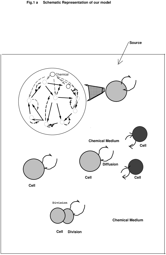
Figure 1: Schematic representation of our model.

Now we come back to the problem of cell differentiation and development. A cell is separated from environment by a membrane, whose separation, however, is not complete. Some chemicals pass through the membrane, and through this transport, cells interact with each other. When a cell is represented by a dynamical system the cells interact with each other and with the external environment. Hence, we need a model consisting of the interplay between inter-unit and intra-unit dynamics. Here we will mainly discuss the developmental process of a cell society accompanied by cell differentiation, where the intra-inter dynamics consist of several biochemical reaction processes. Cells interact through the diffusion of chemicals or their active signal transmission, while they divide into two when some condition is satisfied with the chemical reaction process in it. (See Fig.1 for schematic representation of our model).

We have studied several models[35, 2, 3, 36, 37, 38] with (a) internal (chemical) dynamics of several degrees of freedom, (b) cell-cell interaction type through the medium, and (c) the division to change the number of cells.

As for the internal dynamics, auto-catalytic reaction among chemicals is chosen. Such auto-catalytic reactions are necessary to produce chemicals in a cell, required for reproduction[41]. Auto-catalytic reactions often lead to nonlinear oscillation in chemicals. Here we assume the possibility of such oscillation in the intra-cellular dynamics [42, 43]. As the interaction mechanism, the diffusion of chemicals between a cell and its surroundings is chosen.

To be specific, we mainly consider the following model here. First, the state of a cell $i$ is assumed to be characterized by the cell volume and a set of functions $x^{(m)}_{i}(t)$ representing the concentrations of $k$ chemicals denoted by $m=1,\cdots,k$. The concentrations of chemicals change as a result of internal biochemical reaction dynamics within each cell and cell-cell interactions communicated through the surrounding medium.

For the internal chemical reaction dynamics, we choose a catalytic network among the $k$ chemicals. The network is defined by a collection of triplets ($\ell$,$j$,$m$) representing the reaction from chemical $m$ to $\ell$ catalyzed by $j$. The rate of increase of $x^{\ell}_{i}(t)$ (and decrease of $x^{m}_{i}(t)$) through this reaction is given by $x^{(m)}_{i}(t)(x^{(j)}_{i}(t))^{\alpha}$, where $\alpha$ is the degree of catalyzation ($\alpha=2$ in the simulations considered presently). Each chemical has several paths to other chemicals, and thus a complex reaction network is formed. The change in the chemical concentrations through all such reactions, thus, is determined by the set of all terms of the above type for a given network. (These reactions can include genetic processes).

Cells interact with each other through the transport of chemicals out of and into the surrounding medium. As a minimal case, we consider only indirect cell-cell interactions through diffusion of chemicals via the medium. The transport rate of chemicals into a cell is proportional to the difference in chemical concentrations between the inside and the outside of the cell, and is given by $D(X^{(\ell)}(t)-x^{({\ell})}_{i}(t))$, where $D$ denotes the diffusion constant, and $X^{(\ell)}(t)$ is the concentration of the chemical at the medium. The diffusion of a chemical species through cell membrane should depend on the properties of this species. In this model, we consider the simple case in which there are two types of chemicals, one that can penetrate the membrane and one that cannot. For simplicity, we assume that all the chemicals capable of penetrating the membrane have the same diffusion coefficient, $D$. With this type of interaction, corresponding chemicals in the medium are consumed. To maintain the growth of the organism, the system is immersed in a bath of chemicals through which (nutritive) chemicals are supplied to the cells.

As chemicals flow out of and into the environment, the cell volume changes. The volume is assumed to be proportional to the sum of the quantities of chemicals in the cell, and thus is a dynamical variable. Accordingly, chemicals are diluted as a result of the increase of the cell volume.

In general, a cell divides according to its internal state, for example, as some products, such as DNA or the membrane, are synthesized, accompanied by an increase in cell volume. Again, considering only a simple situation, we assume that a cell divides into two when the cell volume becomes double the original. At each division, all chemicals are almost equally divided, with random fluctuations.

Of course, each result of simulation depends on the specific choice of the reaction network. However, the basic feature of the process to be discussed does not depend on the details of the choice, as long as the network allows for the oscillatory intra-cellular dynamics leading to the growth in the number of cells. Note that the network is not constructed to imitate an existing biochemical network. Rather, we try to demonstrate that important features in a biological system are a natural consequence of a system with internal dynamics, interaction, and reproduction. From the study we try to extract a universal logic underlying a class of biological systems.

7 Scenario for Cell Differentiation

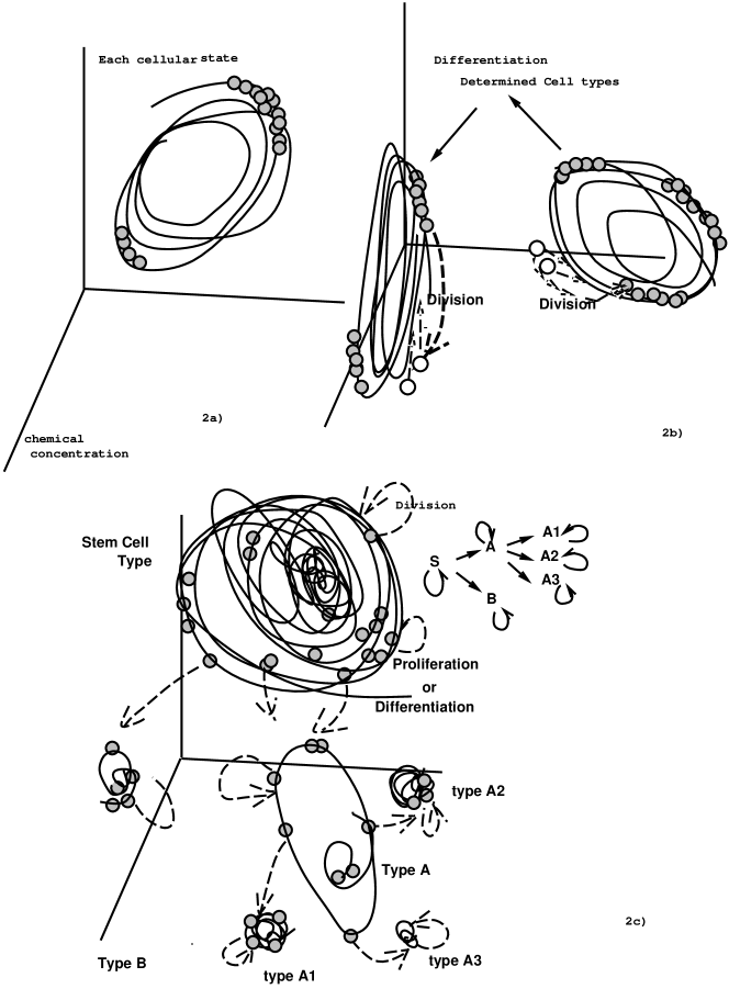
Figure 2: Schematic representation of cell differentiation process, plotted in the phase space of chemical concentrations.

From several simulations of the models starting from a single cell initial condition, we have shown that cells undergo spontaneous differentiation as the number is increased. (see Fig.2 for schematic representation): The first differentiation starts with the clustering of the phase of the oscillations, as discussed in globally coupled maps (see Fig.2a). Then, the differentiation comes to the stage that the average concentrations of the biochemicals over the cell cycle become different. The composition of biochemicals as well as the rates of catalytic reactions and transport of the biochemicals become different for each group.

After the formation of cell types, the chemical compositions of each group are inherited by their daughter cells. In other words, chemical compositions of cells are recursive over divisions. The biochemical properties of a cell are inherited by its progeny, or in other words, the properties of the differentiated cells are stable, fixed or determined over the generations (see Fig. 2b). After several divisions, such initial condition of units is chosen to give the next generation of the same type as its mother cell.

The most interesting example here is the formation of stem cells, schematically shown given in Fig.2c [37]. This cell type, denoted as ‘S’ here, either reproduces the same type or forms different cell types, denoted for example as type A and type B. Then after division events $S\rightarrow S,A,B$ occur. Depending on the adopted chemical networks, the types A and B replicate, or switch to different types. For example $A\rightarrow A,A1,A2,A3$ is observed in some network. This hierarchical organization is often observed when the internal dynamics have some complexity, such as chaos.

The differentiation here is “stochastic”, arising from chaotic intra-cellular chemical dynamics. The choice for a stem cell either to replicate or to differentiate looks like stochastic as far as the cell type is concerned. Since such stochasticity is not due to external fluctuation but is a result of the internal state, the probability of differentiation can be regulated by the intra-cellular state. This stochastic branching is accompanied by a regulative mechanism. When some cells are removed externally during the developmental process, the rate of differentiation changes so that the final cell distribution is recovered.

In some biological systems such as the hematopoietic system, stem cells either replicate or differentiate into different cell type(s). This differentiation rule is often hierarchical [45, 46]. The probability of differentiation to one of the several blood cell types is expected to depend on the interaction. Otherwise, it is hard to explain why the developmental process is robust. For example, when the number of some terminal cells decreases, there should be some mechanism to increase the rate of differentiation from the stem cell to the differentiated cells. This suggests the existence of interaction-dependent regulation of the differentiation ratio, as demonstrated in our results.

Microscopic Stability

The developmental process is stable against molecular fluctuations. First, intra-cellular dynamics of each cell type are stable against such perturbations. Then, one might think that this selection of each cell type is nothing more than a choice among basins of attraction for a multiple attractor system. If the interaction were neglected, a different type of dynamics would be interpreted as a different attractor. In our case, this is not true, and cell-cell interactions are necessary to stabilize cell types. Given cell-to-cell interactions, the cell state is stable against perturbations on the level of each intra-cellular dynamics.

Next, the number distribution of cell types is stable against fluctuations. Indeed, we have carried out simulations of our model, by adding a noise term, considering finiteness in the number of molecules[3, 40]. The obtained cell type as well as the number distribution is hardly affected by the noise as long as the noise amplitude is not too large.

Macroscopic Stability

Each cellular state is also stable against perturbations of the interaction term. If the cell type number distribution is changed within some range, each cellular dynamics keeps its type. Hence discrete, stable types are formed through the interplay between intra-cellular dynamics and interaction. The recursive production is attained through the selection of initial conditions of the intra-cellular dynamics of each cell, so that it is rather robust against the change of interaction terms as well.

The macroscopic stability is clearly shown in the spontaneous regulation of differentiation ratio. How is this interaction-dependent rule formed? Note that depending on the distribution of the other cell types, the orbit of internal cell state is slightly deformed. For a stem cell case, the rate of the differentiation or the replication (e.g., the rate to select an arrow among $S\rightarrow S,A,B$) depends on the cell-type distribution. For example, when the number of “A” type cells is reduced, the orbit of an “S-”type cell is shifted towards the orbits of “A”, with which the rate of switch to “A” is enhanced. The information of the cell-type distribution is represented by the internal dynamics of “S”-type cells, and it is essential to the regulation of differentiation rate [37].

It should be stressed that our dynamical differentiation process is always accompanied by this kind of regulation process, without any sophisticated programs implemented in advance. This autonomous robustness provides a novel viewpoint to the stability of the cell society in multicellular organisms.

8 Dynamical Systems Representations of Cell Differentiation

Since each cell state is realized as a balance between internal dynamics and interaction, one can discuss which part is more relevant to determine the stability of each state. In one limiting case, the state is an attractor as internal dynamics[44], which is sufficiently stable and not destabilized by cell-cell interaction. In this case, the cell state is called ‘determined’, according to the terminology in cell biology. In the other limiting case, the state is totally governed by the interaction, and by changing the states of other cells, the cell state in concern is destabilized. In this case, each cell state is highly dependent on the environment or other cells.

Each cell type in our simulation generally lies between these two limiting cases. To see such intra-inter nature of the determination explicitly, one effective method is a transplantation experiment. Numerically, such experiment is carried out by choosing determined cells (obtained from the normal differentiation process) and putting them into a different set of surrounding cells, to set distribution of cells so that it does not appear through the normal course of development.

When a differentiated and recursive cell is transplanted to another cell society, the offspring of the cell keep the same type, unless the cell-type distribution of the society is strongly biased. When a cell is transplanted into a biased society, differentiation from a ‘determined’ cell occurs. For example, a homogeneous society consisting only of one determined cell type is unstable, and some cells start to switch to a different type. Hence, the cell memory is preserved mainly in each individual cell, but suitable inter-cellular interactions are also necessary to keep it.

Since each differentiated state is not attractor, but is stabilized through the interaction, we propose to define partial attractor, to address attraction restricted to the internal cellular dynamics. Tentative definition of this partial attractor is as follows;

(1) [internal stability] Once the cell-cell interaction is specified (i.e., the dynamics of other cells), the state is an attractor of the internal dynamics. In other words, it is an attractor when the dynamics is restricted only to the variable of a given cell.

(2) [interaction stability] The state is stable against change of interaction term, up to some finite degree. With the change of the interaction term of the order $\epsilon$, the change in the dynamics remains of the order of $O(\epsilon)$.

(3) [self-consistency] For some distribution of units of cellular states satisfying (1) and (2), the interaction term continues to satisfy the condition (1) and (2).

We tentatively call a state satisfying (1)-(3) as partial attractor. Each determined cell type we found can be regarded as a partial attractor. To define the dynamics of stem cell in our model, however, we have to slightly modify the condition of (2) to a ‘Milnor-attractor’ type. Here, small perturbation to the interaction term (by the increase of the cell number) may lead the state to switch to a differentiated state. Hence, instead of (2), we set the condition:

(2’) For some change of interaction with a finite measure, some orbits remain to be attracted to the state.

So far we have discussed the stability of a state by fixing the number of cells. In some case, the condition (3) may not be satisfied when the system is developed from a single cell following the cell division rule. As for developmental process, the condition has to be satisfied for a restricted range of cell distribution realized by the evolution from a single cell. Then we need to add the condition:

(4)[Accessibility]. The distribution (3) is satisfied from an initial condition of a single cell and with the increase of the number of cells.

Cell types with determined differentiation observed in our model is regarded as a state satisfying (1)(2)(3)(4), while the stem cell type is regarded as a state satisfying (1)(2’)(3)(4).

In fact, as the number is increased, some perturbations to the interaction term is introduced. In our model, the stem-cell state satisfies (2) up to some number, but with the further increase of number, the condition (2) is no more satisfied and is replaced by (2’). Perturbation to the interaction term due to the cell number increase is sufficient to bring about a switch from a given stem-cell dynamics to a differentiated cell. Note again that the stem-cell type state with weak stability has a large basin volume when started from a single cell.

9 Towards Biological irreversibility irreducible to thermodynamics

In the normal development of cells, there is clear irreversibility, resulting from the successive loss of multipotency.

In our model simulations, this loss of multipotency occurs irreversibly. The stem-cell type can differentiate to other types, while the determined type that appear later only replicates itself. In a real organism, there is a hierarchy in determination, and a stem cell is often over a progenitor over only a limited range of cell types. In other words, the degree of determination is also hierarchical. In our model, we have also found such hierarchical structure. So far, we have found only up to the second layer of hierarchy in our model with the number of chemicals $k=20$.

Here, the loss of multipotency dynamics of a stem-type cell exhibit irregular oscillations with orbital instability and involve a variety of chemicals. Stem cells with these complex dynamics have a potential to differentiate into several distinct cell types. Generally, the differentiated cells always possess simpler cellular dynamics than the stem cells, for example, fixed-point dynamics and regular oscillations.

Although we have not yet succeeded in formulating the irreversible loss of multipotency in terms of a single fundamental quantity (analogous to thermodynamic entropy), we have heuristically derived a general law describing the change of the following quantities in all of our numerical experiments, using a variety of reaction networks[39, 40]. As cell differentiation progresses through development,

• (I) stability of intra-cellular dynamics increases;

• (II) diversity of chemicals in a cell decreases;

• (III) temporal variations of chemical concentrations decrease, by realizing less chaotic motion.

The degree of (I) could be determined by a minimum change in the interaction to switch a cell state, by properly extending the ‘attractor strength’ in §3. Initial undifferentiated cells spontaneously change their state even without the change of the interaction term, while stem cells can be switched by tiny change in the interaction term. The degree of determination is roughly measured as the minimum perturbation strength required for a switch to a different state.

The diversity of chemicals (II) can be measured, for example, by $S=-\sum_{j=1}^{k}p(j)logp(j)$, with $p(j)=<\frac{x(j)}{\sum_{m=1}^{k}x(m)}>$, with $<..>$ as temporal average. Loss of multipotency in our model is accompanied by a decrease in the diversity of chemicals and is represented by the decrease of this diversity $S$.

The tendency (III) is numerically confirmed by the subspace Kolmorogorv-Sinai (KS) entropy of the internal dynamics for each cell. Here, this subspace KS entropy is measured as a sum of positive Lyapunov exponents, in the tangent space restricted only to the intracellular dynamics for a given cell. Again, this exponent decreases through the development.

10 Discussion: Towards Phenomenology theory of Developmental Process

In the present paper, we have first surveyed some of recent progresses in coupled dynamical systems, in particular globally coupled maps. Then we discuss some of our recent studies on the cell differentiation and development, based on coupled dynamical systems with some internal degrees of freedom and the potentiality to increase the number of units(cells). Stability and irreversibility of the developmental process are demonstrated by the model, and are discussed in terms of dynamical systems.

Of course, results based on a class of models are not sufficient to establish a theory to understand the stability and irreversibility in development of multicellular organisms. We need to unveil the logic that underlies such models and real development universally. Although mathematical formulation is not yet established, supports are given to the following conjecture.

Assume a cell with internal chemical reaction network whose degrees of freedom is large enough and which interacts each other through the environment. Some chemicals are transported from the environment and converted to other chemicals within a cell. Through this process the cell volume increases and the cell is divided. The, for some chemical networks, each chemical state of a cell remains to be a fixed point. In this case, cells remain identical, where the competition for chemical resources is higher, and the increase of the cell number is suppressed. On the other hand, for some reaction networks, cells differentiate and the increase in the cell number is not suppressed. The differentiation of cell types form a hierarchical rule. The initial cell types have large chemical diversity and show irregular temporal change of chemical concentrations. As the number of cells increases and the differentiation progresses, irreversible loss of multipotency is observed. This differentiation process is triggered by instability of some states by cell-cell interaction, while the realized states of cell types and the number distribution of such cell types are stable against perturbations, following the spontaneous regulation of differentiation ratio.

When we recall the history of physics, the most successful phenomenological theory is nothing but thermodynamics. To construct a phenomenology theory for development, or generally a theory for biological irreversibility, comparison with the thermodynamics should be relevant. Some similarity between the phenomenology of development and thermodynamics is summarized in Table 1.

As mentioned, both the thermodynamics and the development phenomenology have stability against perturbations. Indeed, the spontaneous regulation in a stem cell system found in our model is a clear demonstration of stability against perturbations, that is common with the Le Chatelier-Braun principle. The irreversibility in thermodynamics is defined by suitably restricting possible operations, as formulated by adiabatic process. Similarly, the irreversibility in a multicellular organism has to be suitably defined by introducing an ideal developmental process. Note that in some experiments like clone from somatic cells in animals[47], the irreversibility in normal development can be reversed.

The last question that should be addressed here is the search for macroscopic quatities to characterize each (differentiated) cellular ’state’. Although thermodynamics is established by cutting the macroscopic out of microscopic levels, in a cell system, it is not yet sure if such macroscopic quantities can be defined, by separating a macroscopic state from the microscopic level. At the present stage, there is no definite answer. Here, however, it is interesting to recall recent experiments of tissue engineering. By changing the concentrations of only three control chemicals, Asashima and coworkers[48] have succeeded in constructing all tissues from a Xenopus undifferentiated cells (animal cap). Hence there may be some hope that a reduction to a few variables characterizing macroscopic ‘states’ may be possible.

Construction of phenomenology for development charactering its stability and irreversibility is still at the stage ‘waiting for Carnot’, but following our results based on coupled dynamical systems models and some of recent experiments, I hope that such phenomenology theory will be realized in near future.

Table I: Comparison with development phenomenology with thermodynamics

	development phenomenology	thermodynamics
Stability	cellular and ensemble level	macroscopic
stability against perturbation	regulation of differentiation ratio	Le Chatelier Braun
irreversibility	loss of multipotency	second law
quantification of irreversibility	some pattern of gene expression?	entropy
cycle	somatic clone cycle?	Carnot cycle

acknowledgments

The author is grateful to T. Yomo , C. Furusawa, T. Shibata for discussions. The work is partially supported by Grant-in-Aids for Scientific Research from the Ministry of Education, Science, and Culture of Japan.

References

- [1] For pioneering work on development from dynamical systems, see A.M. Turing, The chemical basis of morphogenesis Phil. Trans. Roy . Soc. B 237) (1952) 5
- [2] K. Kaneko and T. Yomo, Bull.Math.Biol. 59 (1997) 139-196
- [3] K. Kaneko and T. Yomo, J. Theor. Biol. (1999) 243-256
- [4] K. Kaneko and I. Tsuda Complex Systems: Chaos and Beyond —–A Constructive Approach with Applications in Life Sciences (Springer, 2000) ( based on K. Kaneko and I. Tsuda Chaos Scenario for Complex Systems (Asakura), 1996, in Japanese)
- [5] K. Kaneko, Prog. Theo. Phys. 72 (1984) 480-486; K.Kaneko ed., Theory and applications of coupled map lattices, Wiley (1993)
- [6] K. Kaneko, Physica 41 D (1990) 137-172
- [7] K. Kaneko Complexity, 3(1998) 53-60
- [8] M. Mezard, G. Parisi, and M.A. Virasoro eds., Spin Glass Theory and Beyond (World Sci. Pub., Singapore, 1988)
- [9] K. Kaneko, Physica D 77 (1994) 456
- [10] K. Kaneko, Physica 75 D (1994) 55
- [11] K. Kaneko, Artificial Life, 1 (1994) 163
- [12] K. Kaneko, J. Phys. A, 24 (1991) 2107
- [13] A. Crisanti, M. Falcioni, and A. Vulpiani, Phys. Rev. Lett. 76 (1996) 612; S.C Manruiba, A. Mikhailov, Europhys. Lett. 53( 2001) 451-457
- [14] K. Kaneko, Phys. Rev. Lett., 78 (1997) 2736-2739; Physica D, 124 (1998) 308-330
- [15] J. Milnor, Comm. Math. Phys. 99 (1985) 177; 102 (1985) 517
- [16] P. Ashwin, J. Buescu, and I. Stuart, Phys. Lett. A 193 (1994) 126; Nonlinearity 9 (1996) 703
- [17] J.C. Sommerer and E. Ott., Nature 365 (1993) 138; E. Ott et al., Phys. Rev. Lett. 71 (1993) 4134
- [18] Y-C. Lai abd R.L.Winslow, Physica D 74 (1994) 353
- [19] I. Tsuda, World Futures 32(1991)167; Neural Networks 5(1992)313
- [20] K. Ikeda, K. Matsumoto, and K. Ohtsuka, Prog. Theor. Phys. Suppl. 99 (1989) 295
- [21] A. Saito and K. Kaneko, “Inaccessibility and Undecidability in Computation, Geometry and Dynamical Systems”, Physica D in press
- [22] T. Konishi and K. Kaneko, J. Phys. A 25 (1992) 6283
- [23] K. Shinjo, Phys. Rev. B 40 (1989) 9167
- [24] K. Kaneko, Phys. Rev. Lett. 65, 1391 (1990); Physica D55, 368 (1992).
- [25] A.S.Pikovsky and J. Kurths, Phys. Rev. Lett. 72 (1994) 1644
- [26] T. Shibata and K. Kaneko, Europhys.Lett., 38 (1997) 417-422
- [27] S. V. Ershov, A. B. Potapov, Physica D86, 532 (1995); Physica D106, 9 (1997).
- [28] T. Chawanya, S. Morita, Physica D116, 44 (1998).
- [29] N. Nakagawa, T. S. Komatsu, Phys. Rev. E 57, 1570 (1998).
- [30] T. Shibata and K. Kaneko Phys. Rev. Lett., 81 (1998) 4116-4119
- [31] T. Shibata, T. Chawanya and K. Kaneko, Phys. Rev. Lett., 82 (1999) 4424-4427
- [32] G. Perez et al., Phys.Rev. A 45 (1992) 5469; S.Sinha et al., Phys Rev. A 46 (1992) 3193
- [33] K. Matsumoto, I. Tsuda, J. Stat. Phys. 31 (1983) 87.
- [34] W. Horsthemke and R. Lefever, Noise-Induced Transitions, edited by H. Haken (Springer, 1984).
- [35] K. Kaneko and T. Yomo, Physica 75 D (1994), 89-102
- [36] K.Kaneko, Physica 103 D(1997) 505-527
- [37] C. Furusawa and K. Kaneko, Bull. Math. Biol., 60 (1998) 659-687
- [38] C. Furusawa and K. Kaneko Artificial Life, 4 (1998) 79-93
- [39] K. Kaneko and C. Furusawa, Physica A 280 (2000) 23-33; C. Furusawa and K. Kaneko Phys. Rev. Lett., 84 (2000) 6130-6133
- [40] C. Furusawa and K. Kaneko, J. Theor. Biol. 209 (2001) 395-416
- [41] M. Eigen and P. Schuster, The hypercycle, Springer Berlin, Heidelberg, N.Y., 1979
- [42] B. Goodwin, “Temporal Organization in Cells” Academic Press, London (1963).
- [43] B. Hess and A. Boiteux, Ann. Rev. Biochem. 40(1971), 237-258
- [44] For a pioneering work to relate cell differentiation with multiple attractors, see S. Kauffman, J. Theo. Biology. 22, (1969) 437
- [45] B. Alberts, D.Bray, J. Lewis, M. Raff, K. Roberts, and J.D. Watson, The Molecular Biology of the Cell, 1989,1994
- [46] M. Ogawa, Blood 81, (1993)2844
- [47] J.B.Gurdon, R.A. Laskey, and O.R. Reeves, Journal of Embryology and Experimental Morphology, 34 (1975) 93-112 ; K.H.S Campbell, J. McWhir, W.A. Ritchie, I. Wilmut, Nature 380 (1996) 64-66
- [48] T. Ariizumi and M Asashima, Int. J. Dev. Biol. 45(2001) 273-279