Event synchronization: a simple and fast method to measure synchronicity and time delay patterns.

Abstract

We propose a simple method to measure synchronization and time delay patterns between signals. It is based on the relative timings of events in the time series, defined e.g. as local maxima. The degree of synchronization is obtained from the number of quasi-simultaneous appearances of events, and the delay is calculated from the precedence of events in one signal with respect to the other. Moreover, we can easily visualize the time evolution of the delay and synchronization level with an excellent resolution.

We apply the algorithm to short rat EEG signals, some of them containing spikes. We also apply it to an intracranial human EEG recording containing an epileptic seizure, and we propose that the method might be useful for the detection of foci and for seizure prediction. It can be easily extended to other types of data and it is very simple and fast, thus being suitable for on-line implementations.

I Introduction

In recent years, several measures of synchronization have been proposed and applied successfully to different types of data. Among these studies we can distinguish two main approaches: 1) One based on similarities of trajectories in phase space (constructed e.g. by time-delay embedding) schiff ; quyen ; arnhold ; quian ; quian1 ; 2) One that measures phase differences between the signals, where the phases are defined either from a Hilbert rosemblum ; tass ; florian or from a wavelet transform lachaux ; rodriguez (as shown in quian1 , these two apparently different phases are indeed closely related).

These new methods compete in popularity with standard measures such as the cross-correlation, the coherence function, mutual information, and also with simple visual inspection of the recordings. Cross-correlation and coherence are clearly the measures most used so far. In contrast to them, all new measures are non-linear in the sense that they depend also on properties beyond second moments. In addition, some of them have the advantage of being asymmetric, eventually being able to show driver-response relationships arnhold ; quian .

Among others, synchronization measures have been used for the study of electroencephalogram (EEG) signals. Applications include prediction and localization of epileptic activity quyen ; arnhold ; florian , phase-locking between different recording sites upon visual stimulation lachaux ; rodriguez , resonance between EEG and muscle activity in Parkinson patients tass , desynchronization upon lesions in the thalamic reticular nucleus in rats sleepwake , synchronization in motoneurons within the spinal cord schiff , etc.

In the present paper we present a very simple algorithm that can be used for any time series in which we can define events. These can be spikes in single-neuron recordings, epileptiform spikes in EEGs, heart beats, stock market crashes, etc. In principle, when dealing with signals of different character, the events could be defined differently in each time series, since their common cause might manifest itself differently in each series. This event synchronization (ES) does not require the notion of phase. It cannot distinguish between different forms of $m:n$ lockings rosemblum ; tass , but it can tell which of the two time series leads the other. And, above all, it is very simple conceptually and easy to implement. Due to that, it can be used on-line and can show rapid changes of synchronization patterns.

II Event synchronization and delay asymmetry

Given two simultaneously measured discrete univariate time series $x_{n}$ and $y_{n}$, $n=1,\ldots,N$, we first define suitable events and event times $t^{x}_{i}$ and $t^{y}_{j}$ $(i=1,\ldots,m_{x};j=1,\ldots,m_{y})$. In the signals to be analyzed in this paper, these events will be simply local maxima, subject to some further conditions. If the signals are synchronized, many events will appear more or less simultaneously. Essentially, we count the fraction of event pairs matching in time, and we count how often each time series leads in these matches. Similar concepts were used in pijn .

Let us first assume that there is a well defined characteristic event rate in each time series. Counter examples include strong chirps and onsets of epileptic seizures where event rates change rapidly. Such cases will be treated below. Allowing a time lag $\pm\tau$ between two ‘synchronous’ events (which should be smaller than half the minimum inter-event distance, to avoid double counting), let us denote by $c^{\tau}(x|y)$ the number of times an event appears in $x$ shortly after it appears in $y$, i.e:

$$c^{\tau}(x|y)=\sum_{i=1}^{m_{x}}\sum_{j=1}^{m_{y}}J_{ij}^{\tau}$$ (1)

with

$$J_{ij}^{\tau}=\cases{1&if ~{}~{}$0<t_{i}^{x}-t_{j}^{y}\leq\tau$\cr 1/2&if ~{}~{}$t^{x}_{i}=t^{y}_{j}$\cr 0&else}$$ (2)

and analogously for $c^{\tau}(y|x)$. Next, we define the symmetrical and anti-symmetrical combinations

$$Q_{\tau}=\frac{c^{\tau}(y|x)+c^{\tau}(x|y)}{\sqrt{m_{x}m_{y}}}\ ,\quad q_{\tau}=\frac{c^{\tau}(y|x)-c^{\tau}(x|y)}{\sqrt{m_{x}m_{y}}}\ ,$$ (3)

which measure the synchronization of the events and their delay behavior, respectively. They are normalized to $0\leq Q_{\tau}\leq 1$ and $-1\leq q_{\tau}\leq 1$. We have $Q_{\tau}=1$ if and only if the events of the signals are fully synchronized. In addition, if the events in $x$ always precede those in $y$, then $q_{\tau}=1$.

In cases where we want to avoid a global time scale $\tau$ since event rates change during the recording, we use a local definition $\tau_{ij}$ for each event pair $(ij)$. More precisely, we define

$$\tau_{ij}=\min\{t^{x}_{i+1}-t^{x}_{i},t^{x}_{i}-t^{x}_{i-1},t^{y}_{j+1}-t^{y}_{j},t^{y}_{j}-t^{y}_{j-1}\}\,/2\;.$$ (4)

We then define $J_{ij}$ as in Eq.(2) with $\tau$ replaced by $\tau_{ij}$, and $c(x|y)$ as in Eq.(1) with $J_{ij}^{\tau}$ replaced by $J_{ij}$. The factor $1/2$ in the definition of $\tau_{ij}$ avoids double counting if, e.g., two events in $x$ are close to the same event in $y$. Of course, one could also make other choices, e.g. by taking $\tau_{ij}$ smaller than in Eq.(4) or by using $\tau^{\prime}_{ij}=\min\{\tau,\tau_{ij}\}$. As in the definition of events, an optimal choice of $\tau$ depends on the problem. In the following we shall suppress the dependence on $\tau$, understanding that all formulas apply for both variants.

To obtain time resolved variants of $Q$ and $q$ we simply modify eq.(1) to

$$c_{n}(x|y)=\sum_{i}\sum_{j}J_{ij}\,\Theta(n-t_{i}^{x})$$ (5)

with $n=1,\ldots,N$ and $\Theta$ the step function (i.e. $\Theta(x)=0$ for $x\leq 0$ and $\Theta(x)=1$ for $x>0$). Similarly, $c_{n}(y|x)$ is obtained by exchanging $x$ and $y$. Then, we define the time resolved anti-symmetric combination $q(n)=c_{n}(y|x)-c_{n}(x|y)$ which can be seen as a random walk that takes one step up every time an event in $x$ precedes one in $y$ and one step down if vice versa. If an event occurs simultaneously in both signals or if it appears only in one of them, the random walker does not move. Exchanging $x$ and $y$ just reverses the walk. For non-synchronized signals, we expect to obtain a random walk with the typical diffusion behavior. With delayed synchronization we will have a bias going up (down) if $x$ precedes (follows) $y$. We should remark that such a bias clearly shows the presence of a time delay of one signal with respect to the other, but does not necessarily prove a driver-response relationship, although it might suggest it. In fact, internal delay loops of one of the systems can fool the interpretation. Also, the two signals might be driven by a common hidden source and the bias just indicates different delays.

The time course of the strength of ES can be obtained from $Q(n)=c_{n}(y|x)+c_{n}(x|y)$. If an event is found both in $x$ and $y$ within the window $\tau$ (resp. $\tau_{ij}$), $Q(n)$ increases one step, otherwise it does not change. Of course, $Q(n)$ will also not change if there are no new events at all. The synchronization level at time $n$, averaged over the last $\Delta n$ time steps, is thus obtained as

$$Q^{\prime}(n)={Q(n)-Q(n-\Delta n)\over\sqrt{\Delta n_{x}\Delta n_{y}}}\;,$$ (6)

where $\Delta n_{x}$ and $\Delta n_{y}$ are the numbers of events in the interval $[n-\Delta n,n]$. Similarly, we can also define instantaneous delay asymmetries $q^{\prime}(n)$.

III Applications

Let us now apply these concepts to two sets of intracranial EEG recordings, one from rats and the other from an epileptic patient.

III.1 Rat EEGs

The five pairs of rat EEG signals were obtained from electrodes placed on the left and right frontal cortex of male adult WAG/Rij rats (a genetic animal model of human epilepsy) giles . They were referenced to an electrode placed in the cerebellum, filtered between 1-100 Hz and digitized at 200 Hz. In Fig. 1 we show these signals www . The first pair (example A in Fig. 1) is a normal EEG, all others contain spike discharges (not to be confused with spikes in single neuron recordings) which are the landmark of epileptic activity. They arise from abnormal synchronization in an epileptic brain even when there are no seizures. A localized appearance of spikes can indeed delimit a zone with abnormal activity (though this will not necessarily be the epileptic focus). Furthermore, time delays between them can identify the electrode closest to the epileptic focus, especially at the onset of seizures.

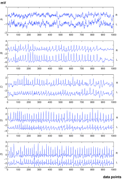
Figure 1: Five pairs of rat EEG signals from right and left cortical intracranial electrodes. For a better visualization, left signals are plotted with an offset.

Several measures of synchronization were recently applied to the first three cases of Fig. 1 quian1 . Since spike trains lasted usually about 5 seconds, the challenge was to try the different measures in these short epochs. Surprisingly, nearly all the measures gave qualitatively similar results hard to be guessed beforehand. These examples and two additional cases (D and E), also containing spikes, will be further analyzed in this paper.

For the example A it is difficult, due to its random-like appearance, to visually estimate its level of synchronization and any delay of one electrode with respect to the other. However, we can already observe some patterns appearing nearly simultaneously in both the left and right channels, thus showing some degree of interdependence. The spike-wave trains in the other examples in principle suggests a high level of synchronization. However, as already shown in quian1 , the spikes of example C appear with a varying time lag between right and left channels and are therefore much less synchronized than those in B. This is of course not easily seen by visual inspection of Fig. 1, but will be clear from the following analysis.

Events were defined as local maxima fulfilling the following additional conditions:

1. $x(t_{i})>x(t_{i+k})$, for $k=-K+1,\ldots,0,\ldots,K-1$

2. $x(t_{i})>x(t_{i\pm K})+h$

and the same for $y$. We took $K=3$ and $h=0.1$. Other choices gave very similar results.

Since the rate of events is more or less constant, we used a fixed $\tau$. The choice $\tau=2$ gave a good discrimination between the five cases. All results shown below were compared to those obtained with surrogate pairs which were defined by shifting the left channel signals 500 data points (2.5 sec) to the right, with periodic boundary conditions. Our test hypothesis is that without changing the individual properties of each signal, after a large enough shifting synchronization should reach a background ‘zero’ level. The usefulness of such surrogates was discussed in in more detail in quian1 .

Example	$Q_{\tau=2}$	$q_{\tau=2}$	$Q_{\tau=2}^{{}^{\rm surr}}$	$q_{\tau=2}^{{}^{\rm surr}}$
A	0.57	0.15	0.24	-0.01
B	0.80	-0.29	0.29	0.01
C	0.48	-0.20	0.13	-0.01
D	0.93	-0.59	0.41	0.04
E	0.90	-0.13	0.46	0.03

Table 1: Time averaged event synchronization $Q$ and delay $q$ for the five examples of Fig. 1. Positive values of $q$ indicate that events in the left side lags behind the right one. Surrogate values of synchronization were obtained by shifting left channel signals by 500 data points.

For the five EEG signals of Fig. 1, we show the values of $Q_{\tau=2}$ and $q_{\tau=2}$ in Table 1, both for the original signals and the ‘time-shifted’ surrogates. We observe that synchronization levels rank ${\rm D>E>B>A>C}$. This is in agreement with the analysis of examples A, B and C done in quian1 with several other measures of synchronization. Note that even example A is ranked consistently with the other measures, although it does not contain obvious events such as the spikes of the other examples.

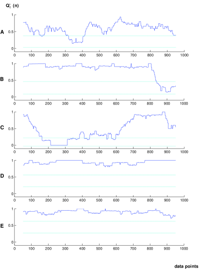
Figure 2: Time resolved event synchronization $Q^{\prime}_{\tau=2}(n)$ for the examples of Fig. 1. Blue horizontal lines correspond to the time averages $\pm 1\sigma$ of the surrogate.

All synchronization values are clearly higher than those of their corresponding surrogates (surrogates constructed with other delay values gave similar results). These surrogate values vary a lot for the different examples. This stresses the importance of keeping the individual properties of the signals when constructing surrogates. Except for example A, the values of $q$ show that the signals from the right hemisphere lag behind the left ones ($y$). A closer visual inspection of Fig. 1 at higher resolution shows that this lag is usually 1 data point. The reason of this systematic lag is unclear (it could be an artifact of the data acquisition or a real physiological effect) and it is beyond the scope of this paper.

In Fig. 2 we show the time evolution of synchronization $Q^{\prime}(n)$ for the five examples, calculated with a window of $\Delta n=100$ data points. For most of the time, they are higher than the values calculated from time-shifted surrogates (the light blue horizontal lines indicate time averages $\pm 1$ standard deviation). In examples A, B and C we see abrupt changes of synchronization with time which seem statistically significant. In retrospect they can also be seen in Fig. 1 on closer inspection, but they are much less obvious there and could easily be missed. Compared to the first three, examples D and E are more stable in time. Finally, the time resolved ES shows a better resolution than all synchronization measures considered in quian1 .

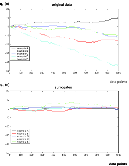
Figure 3: Time delays between the right and left channels (upper plot) and for the surrogates (lower plot). Up (down) shifts mean precedence of the right (left) channel.

Figure 3 shows the time resolved asymmetry between the right and the left channels (upper plot) and the results from surrogates (lower plot). In all five cases, the bias is in agreement with the $q$ values shown in Table 1. The bias in example D is not only the strongest but also the most constant, confirming that D shows the most robust and stationary ES (compare Fig. 2). For the other examples we see regular changes with time. This is of course very difficult to see in the original recordings, and it was also not seen with any of the synchronization measures studied in quian1 . As expected, for the surrogates we obtain random walks with small and erratic displacements.

III.2 Human EEG

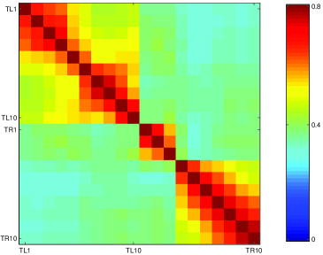
Figure 4: Time averaged event synchronization between the contacts on the left and right depth electrodes (TL1-10 and TR1-10, respectively).

As a second example we analyzed an intracranial EEG recording from an epileptic patient containing 12 min. of pre-seizure and seizure EEG. Data were recorded from 2 needle shaped depth electrodes with 10 contacts each. They were symmetrically placed in the left (contacts TL1 to TL10) and right (contacts TR1 to TR10) temporal lobes, in the entorhinal cortex and hippocampal formation. The EEG was sampled at 173 Hz and band pass filtered between 0.53-40 Hz. For further details on the data we refer to arnhold . As in the previous example, event times were defined as local maxima, but using $K=10$ and $h=50$ (this large $K$ was needed because the data are more noisy than the rat data, and smaller values would have led to many spurious events). Due to the varying event rate, we used a variable-$\tau$ approach. For the time resolved event synchronization $Q^{\prime}(n)$ we took a window $\Delta n=1730$.

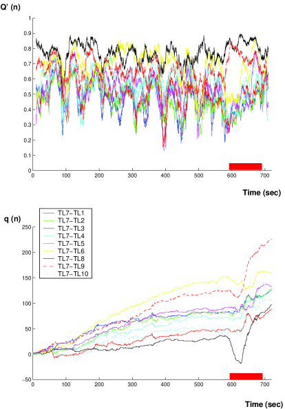
Figure 5: Time resolved event synchronization (upper plot) and delay asymmetries (lower plot) between an channel near the epileptic focus (TL7) and the remaining channels on the same side. The red bar shows the duration of the epileptic seizure.

Figure 4 shows the time-averaged event synchronization values between all channels. A detailed analysis of synchronization patterns for similar recordings has already been described by Arnhold et al. arnhold using a robust measure of non-linear synchronization. Here, we just summarize the main results which are in perfect agreement with those in Ref. arnhold . We first note that synchronization between left and right electrodes is relatively low and that the right contacts form two clusters: TR1-3 and TR4-10. This is just due to the fact that the first 3 contacts were located in the entorhinal cortex and the remaining ones in the hippocampus arnhold . Moreover, for the right side we observe a gradual decrease of synchronization with increasing distance between contacts. The synchronization pattern for the left channels is different. There, the entorhinal cortex/hippocampus separation is overshadowed by the epileptic activity leading to a higher overall synchronization level.

A visual analysis of the seizure onset revealed that contacts TL7 and TL8 showed the first signs of seizure activity. Figure 5 shows the time resolved synchronization $Q^{\prime}(n)$ and delays $q(n)$ between TL7 and the remaining left side channels. As expected, synchronization is largest between TL7 and its neighbors TL8 and TL6. It is not homogeneous in time and we have several short drops before seizure starts. Moreover, starting at seizure onset and during the whole seizure, synchronization of TL7 with TL8 and TL9 is high, while synchronization with TL6 and all others is decreased. The lower panel shows that all left channels lag behind channel TL7. There is just one exception: During the first part of the seizure, channel TL7 falls back and channel TL8 leads for about half a minute (indeed, the lead of TL7 is weakened already some 3 minutes before the seizure). After this, TL7 takes up its lead even more vigorously than before. This might indicate that the source of epileptic activity moves. Whether these features are common to many epileptic seizures and whether they can have clinical significance for e.g. seizure anticipation or focus localization requires further study with a larger database.

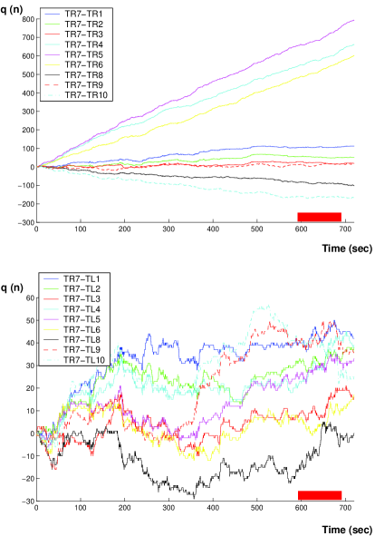
Figure 6: Delay patterns between an contact in the non-focal side (TR7) against the other contacts in the non-focal side (upper plot) and against the contacts in the focal side (lower plot). No anomalous behavior is seen during the seizure (red bar). Notice the different scales in the two plots.

In Fig. 6 we show the delays of the contralateral channel (TR7) with respect to the other right channels (upper plot) and to the left channels (lower plot). Channels TR4-6 strongly and steadily follow channel TR7, which itself follows channels TR8 and TR10. This might reflect the source of ‘normal’ synchronized activity. A detailed analysis is outside the scope of this paper and will be further addressed elsewhere. As seen from the lower panel, synchronization between both hemispheres is weak and $q$ shows unbiased random walks. The complete absence of any deviant behavior during the seizure reflects the fact that the seizure does not spread to the contralateral side.

IV Conclusion

In conclusion we presented a new approach to measure synchronization and time delays that is based on the relative timings of events (in this study defined as local maxima). This also gives an easy visualization of time-resolved synchronization and delay patterns. The method is appealing due to its simplicity, straightforward implementation and speed. These features make very easy its on-line implementation. In the particular case of EEGs, the proposed approach is promising for the study of recordings of epileptic patients, where synchronization is important and the analysis of time delay patterns could be useful for the localization of the epileptic focus and the prediction of seizure onset. Also, the method should be well suited for single-neuron recordings, where the fast dynamics of spikes makes difficult the analysis with other measures. In this paper we focussed on application to EEG signals, but the method can be easily applied to other types of data just by adjusting the definition of events.

We are very thankful to Ralph Andrzejak, Alexander Kraskov, Klaus Lehnertz, and Heinz Schuster for stimulating discussions, to Giles van Luijtelaar and Joyce Welting from NICI, University of Nijmegen, for the rats data used in this paper and to K. Lehnertz and C. Elger from the Department of Epileptology, University of Bonn, for the intracranial EEG data. T.K. is supported by the Deutsche Forschungsgemeinschaft, SFB TR3.

References

- (1) S.J. Schiff, P. So, T. Chang, R.E. Burke and T. Sauer, Phys. Rev. E 54, 6708 (1996).
- (2) M. Le Van Quyen, J. Martinerie, C. Adam, and F.J. Varela, Physica D 127, 250 (1999).
- (3) J. Arnhold, P. Grassberger, K. Lehnertz, and C.E. Elger, Physica D 134, 419 (1999).
- (4) R. Quian Quiroga, J. Arnhold and P. Grassberger, Phys. Rev. E, 61, 5142 (2000).
- (5) R. Quian Quiroga, A. Kraskov, T. Kreuz and P. Grassberger, Phys. Rev. E, in press.
- (6) M. Rosenblum, A. Pikovsky and J. Kurths, Phys. Rev. Lett, 76, 1804 (1996).
- (7) P. Tass, M. Rosenblum, J. Weule, J. Kurths, A. Pikovsky, J. Volkmann, A. Schitzler and H. Freund, Phys. Rev. Lett, 81, 3291 (1998).
- (8) F. Mormann, K. Lehnertz, P. David and C.E. Elger, Physica D, 144, 358 (2000).
- (9) J. Lachaux, E. Rodriguez, J. Martinerie and F. Varela, Human Brain Mapping, 8, 194 (1999).
- (10) E. Rodriguez, N. George, J. Lachaux, J. Martinerie, B. Renault and F. Varela, Nature, 397, 430 (1999).
- (11) G. van Luijtelaar, J. Welting and R. Quian Quiroga, in: van Bemmel et al. (eds.) Sleep-wake research in the Netherlands, vol 11, pp:86-95 (Dutch Society for Sleep-Wake Research, 2000).
- (12) J.P.M. Pijn, Quantitative Evaluation of EEG Signals in Epilepsy, PhD. Thesis, Amsterdam University (1990)
- (13) G. van Luijtelaar and A. Coenen (eds.), The WAG/Rij rat model of absence epilepsy: Ten years of research (Nijmegen University Press, 1997).
-
(14)
The EEG signals can be downloaded from
www.vis.caltech.edu/~rodrigo.