Wave Structures and Nonlinear Balances in a Family of 1+1 Evolutionary PDEs

Abstract

We introduce the following family of evolutionary 1+1 PDEs that describe the balance between convection and stretching for small viscosity in the dynamics of 1D nonlinear waves in fluids:

$$m_{t}\ +\ \underbrace{\ \ um_{x}\ \ }_{\hbox{convection}}\ +\ \underbrace{\ \ b\,u_{x}m\ \ }_{\hbox{stretching}}\ =\ \underbrace{\ \ \nu\,m_{xx}\ }_{\hbox{viscosity}}\,,\quad\hbox{with}\quad u=g*m\,.$$

Here $u=g*m$ denotes $u(x)=\int_{-\infty}^{\infty}g(x-y)m(y)\,dy\,.$ This convolution (or filtering) relates velocity $u$ to momentum density $m$ by integration against the kernel $g(x)$. We shall choose $g(x)$ to be an even function, so that $u$ and $m$ have the same parity under spatial reflection. When $\nu=0$, this equation is both reversible in time and parity invariant. We shall study the effects of the balance parameter $b$ and the kernel $g(x)$ on the solitary wave structures, and investigate their interactions analytically for $\nu=0$ and numerically for small viscosity, $\nu\neq 0$.

This family of equations admits the classic Burgers “ramps and cliffs” solutions which are stable for $-1<{b}<1$ with small viscosity.

For $b<-1$, the Burgers ramps and cliffs are unstable. The stable solution for $b<-1$ moves leftward instead of rightward and tends to a stationary profile. When $m=u-\alpha^{2}u_{xx}$ and $\nu=0$, this profile is given by $u(x)\simeq{\rm sech}^{2}(x/(2\alpha))$ for $b=-2$, and by $u(x)\simeq{\rm sech}(x/\alpha)$ for $b=-3$.

For $b>1$, the Burgers ramps and cliffs are again unstable. The stable solitary traveling wave for $b>1$ and $\nu=0$ is the “pulson” $u(x,t)=cg(x-ct)$, which restricts to the “peakon” solution in the special case $g(x)=e^{-|x|/\alpha}$ when $m=u-\alpha^{2}u_{xx}$. Nonlinear interactions among these pulsons or peakons are governed by the superposition of solutions for $b>1$ and $\nu=0$,

$$u(x,t)=\sum_{i=1}^{N}p_{i}(t)\,g(x-q_{i}(t))\,.$$

These solutions obey a finite dimensional dynamical system for the time-dependent speeds $p_{i}(t)$ and positions $q_{i}(t)$. We study the pulson and peakon interactions analytically, and we determine their fate numerically under adding viscosity.

1 Introduction

1.1 The b-family of fluid transport equations

We shall analyze a one-dimensional version of active fluid transport that is described by the following family of 1+1 evolutionary equations,

$$m_{t}\ +\ \underbrace{\ \ um_{x}\ \ }_{\hbox{convection}}\ +\ \underbrace{\ \ b\,u_{x}m\ \ }_{\hbox{stretching}}\ =\ 0\,,\quad\hbox{with}\quad u=g*m\,,$$ (1)

in independent variables time $t$ and one spatial coordinate $x$.

We shall seek solutions for the fluid velocity $u(x,t)$ that are defined either on the real line and vanishing at spatial infinity, or on a periodic one-dimensional domain. Here $u=g*m$ denotes the convolution (or filtering),

$$u(x)=\int_{-\infty}^{\infty}g(x-y)m(y)\,dy,$$ (2)

which relates velocity $u$ to momentum density $m$ by integration against kernel $g(x)$ over the real line. We shall choose $g(x)$ to be an even function, so that $u$ and $m$ have the same parity.

The family of equations (1) is characterized by the kernel $g$ and the real dimensionless constant $b$, which is the ratio of stretching to convective transport. As we shall see, $b$ is also the number of covariant dimensions associated with the momentum density $m$. The function $g(x)$ will determine the traveling wave shape and length scale for equation (1), while the constant $b$ will provide a balance or bifurcation parameter for the nonlinear solution behavior. Special values of $b$ will include the first few positive and negative integers.

The quadratic terms in equation (1) represent the competition, or balance, in fluid convection between nonlinear transport and amplification due to $b-$dimensional stretching. For example, if $m$ is fluid momentum (a one-form density in one dimension) then $b=2$. Equation (1) with $b=2$ arises in the nonlinear dynamics of shallow water waves, as shown in [2] and [6]. Equation (1) with $b=2$ and $b=3$ appears in the theory of integrable partial differential equations [2, 6, 4]. The three-dimensional analog of equation (1) with $b=2$ was introduced in [8, 9]. Applying the proper viscosity to this three-dimensional analog with $b=2$ produces the Navier-Stokes-alpha model of turbulence [3]. The 1D version of this turbulence model is

$$m_{t}\ +\ \underbrace{\ \ um_{x}\ \ }_{\hbox{convection}}\ +\ \underbrace{\ \ b\,u_{x}m\ \ }_{\hbox{stretching}}\ =\ \underbrace{\ \ \nu\,m_{xx}\ }_{\hbox{viscosity}}\,,\quad\hbox{with}\quad u=g*m\,.$$ (3)

We shall compare our analysis of equation (1) with numerical simulations of (3) for small viscosity.

1.2 Outline of the paper

After summarizing previous investigations of particular cases in the b-family (1) of active transport equations, section 2 discusses its symmetries and other general properties such as parity and reversibility. Section 3 discusses the traveling waves of equation (1) and derives their Pulson solutions, which may be generalized functions for $b>1$. Section 4 analyzes the interaction dynamics of the Pulson solutions for any positive $b$ and any $g$. Section 5 specializes the analysis of the Pulson solutions to the Peakons, for which $g(x)=e^{-|x|/\alpha}$ is a peaked pulse of width $\alpha$, and $b$ is taken to be arbitrary. In section 6 we add viscosity to the peakon equation, and describe our numerical methods for illustrating the different types of behavior that may arise in the initial value problems for Peakon solutions with $b>0$, $b=0$ and $b<-1$. Section 7 using these numerical methods to determine how viscosity affects the fate of the peakons. Section 8 provides a synopsis of the figures. Section 9 summarizes the paper’s main conclusions.

2 History and general properties of the b-equation

Camassa and Holm [2] derived the following equation for unidirectional motion of shallow water waves in a particular Galilean frame,

$$m_{t}\ +\underbrace{\ \ um_{x}\ \ }_{\hbox{convection}}\ +\ \underbrace{\ \ 2\,u_{x}m\ \ }_{\hbox{stretching}}\ =\ \underbrace{-\,c_{0}u_{x}-\,\gamma\,u_{xxx}\ }_{\hbox{dispersion}}\quad\&\quad m=u-\alpha^{2}u_{xx}\,.$$ (4)

Here $m=u-\alpha^{\,2}u_{xx}$ is a momentum variable, partial derivatives are denoted by subscripts, the constants $\alpha^{\,2}$ and $\gamma/c_{0}$ are squares of length scales, and $c_{0}=\sqrt{g^{\prime}h}$ is the linear wave speed for undisturbed water of depth $h$ at rest under gravity $g^{\prime}$ at spatial infinity, where $u$ and $m$ are taken to vanish. Any constant value $u=u_{0}$ is also a solution of (4).

Equation (4) was derived using Hamiltonian methods in [2] and was shown in [6] also to appear as a water wave equation at quadratic order in the standard asymptotic expansion for shallow water waves in terms of their two small parameters (aspect ratio and wave height). The famous Korteweg-de Vries (KdV) equation appears at linear order in this asymptotic expansion and is recovered from equation (4) when $\alpha^{2}\to 0$. Both KdV at linear order and its nonlocal, nonlinear generalization in equation (4) at quadratic order in this expansion have the remarkable property of being completely integrable by the isospectral transform (IST) method. The IST properties of KdV solitons are well known and these properties for equation (4) were studied in, e.g., [2] and [1].

When linear dispersion is absorbed by a Galilean transformation and a velocity shift, equation (4) reduces to an active transport equation that contains competing quadratically nonlinear terms representing convection and stretching,

$$m_{t}\ +\ \underbrace{\ \ um_{x}\ \ }_{\hbox{convection}}\ +\ \underbrace{\ \ 2\,u_{x}m\ \ }_{\hbox{stretching}}\ =\ 0\,,\quad\hbox{with}\quad m=u-\alpha^{2}u_{xx}\,.$$ (5)

This is a special case of equation (1) for which $b=2$ and $g(x)=e^{-|x|/\alpha}$. The traveling wave solution of (5) is the “peakon,” $u(x,t)=ce^{-|x-ct|/\alpha}$ found in [2], where $e^{-|x|/\alpha}$ is the Green’s function for the Helmholtz operator that relates $m$ and $u$. The interactions among $N$ peakons are governed by the $2N$ dimensional dynamical system for the speeds $p_{i}(t)$ and positions $q_{i}(t)$ $i=1,\dots,N,$ appearing in the solution,

$$u(x,t)=\sum_{i=1}^{N}p_{i}(t)\,e^{-|x-q_{i}(t)|}\,.$$ (6)

As shown in Camassa and Holm [2], a closed integrable Hamiltonian system of ordinary differential equations for the speeds $p_{i}(t)$ and positions $q_{i}(t)$ results upon substituting the superposition of peakons (6) into equation (5). This integrable system governs the dynamics of the peakon interactions.

A variant of equation (5) with coefficient $b=2\to{b}=3$,

$$m_{t}\ +\ \underbrace{\ \ um_{x}\ \ }_{\hbox{convection}}\ +\ \underbrace{\ \ 3\,u_{x}m\ \ }_{\hbox{stretching}}\ =\ 0\,,\quad\hbox{with}\quad m=u-\alpha^{2}u_{xx}\,,$$ (7)

was first singled-out for further analysis by Degasperis and Procesi [5]. Degasperis, Holm and Hone [4] discovered that this $2\to 3$ variant of equation (5) possesses superposed peakon solutions (6) and also is completely integrable by the isospectral transform method. Thus, the $N-$dimensional pulson solution (6) is a completely integrable dynamical system for (7), as well, but with different dynamics for the speeds $p_{i}(t)$ and positions $q_{i}(t)$ of the peakons.

Fringer and Holm [7] extended the zero-dispersion equation (5) for the peakons to the “pulson” equation,

$$m_{t}\ +\ \underbrace{\ \ um_{x}\ \ }_{\hbox{convection}}\ +\ \underbrace{\ \ 2\,u_{x}m\ \ }_{\hbox{stretching}}\ =\ 0\,,\quad\hbox{with}\quad u=g*m\,.$$ (8)

Here $u=g*m$ denotes the convolution (or filtering)

$$u(x)=\int_{-\infty}^{\infty}g(x-y)m(y)\,dy\,,$$ (9)

that relates velocity $u$ to momentum density $m$ by integration against the kernel $g(x)$. Fringer and Holm [7] chose $g(x)$ to be an even function, so that $u$ and $m$ have the same parity. They studied the effects of the shape of the traveling wave $u(x,t)=cg(x-ct)$ on its interactions with other traveling waves in the superposed solution,

$$u(x,t)=\sum_{i=1}^{N}p_{i}(t)\,g(x-q_{i}(t))\,,$$ (10)

This superposed solution of traveling wave forms with time dependent speeds $p_{i}(t)$ and positions $q_{i}(t)$, $i=1,\dots,N,$ revealed that the nonlinear interactions among these pulsons occur by elastic two-pulson scattering, even though the Fringer-Holm pulson equation (8) is not integrable for an arbitrary choice of the kernel $g$. When $g(x)=e^{-|x|/\alpha}$ is assumed, the pulson equation for $b=2$ in (8) specializes to the peakon equation for $b=2$ in (5).

2.1 Discrete symmetries: reversibility, parity and signature

Equation (1) for $m$ is reversible, or invariant under $t\to-t$ and $u\to-u$. The latter implies $m\to-m$. Hence, the transformation $u(x,t)\to-u(x,-t)$ takes solutions into solutions, and in particular, it reverses the direction and amplitude of the traveling wave $u(x,t)=cg(x-ct)$.

We choose $g(x)$ to be an even function so that $m$ and $u=g*m$ both have odd parity under mirror reflections. Hence, equation (1) is invariant under the parity reflections $u(x,t)\to-\,u(-x,t)$, and the solutions of even and odd parity form invariant subspaces.

Equation (1) implies a similar reversible, parity invariant equation for the absolute value $|m|$,

$$|m|_{t}+\,u|m|_{x}+b\,u_{x}|m|=0\,,\quad\hbox{with}\quad u=g*m\,.$$ (11)

So, the positive and negative components $m_{\pm}=\frac{1}{2}(m\pm|m|)$ satisfy equation (1) separately. Also, if $m$ is initially zero, it remains so. This is conservation of the signature of $m$.

2.2 Lagrangian representation

If $m^{1/b}$ is well-defined, equation (1) may be written as the conservation law

$$\partial_{t}\,m^{1/b}+\partial_{x}(m^{1/b}u)=0\,,$$ (12)

and equation (11) for the absolute value implies

$$\partial_{t}\,|m|^{1/b}+\partial_{x}(|m|^{1/b}u)=0\,.$$ (13)

Adding and subtracting equations (12) and (13) implies

$$\partial_{t}\,(m^{1/b})_{\pm}+\partial_{x}\big{(}(m^{1/b})_{\pm}u\big{)}=0\quad\hbox{with}\quad(m^{1/b})_{\pm}=\frac{1}{2}(m^{1/b}\pm|m|^{1/b})\,.$$ (14)

Consequently, regions of positive and negative $m$ are transported by the same velocity and their boundaries propagate so as to separately preserve the two integrals,

$$\int_{-\infty}^{\infty}(m^{1/b})_{\pm}\,dx\,.$$ (15)

The common transport velocity allows a transformation to Lagrangian coordinates $X_{\pm}$ defined by

$$dX_{\pm}=(m^{1/b})_{\pm}(dx-udt)\quad\hbox{so that}\quad\partial_{t}X_{\pm}+u\partial_{x}X_{\pm}=0\,.$$ (16)

This formal transformation is not strictly defined where $(m^{1/b})_{\pm}$ vanishes. However, by equation (14), regions where $(m^{1/b})_{\pm}$ vanishes do not propagate and do not contribute to the integrated value of $X_{\pm}=\int_{-\infty}^{x}(m^{1/b})_{\pm}(y,0)\,dy$. Hence, these regions may be identified and excluded initially. The formal inverse relation holding in the remaining regions,

$$dx=(m^{1/b})_{\pm}^{-1}\,dX_{\pm}+udt\,,$$ (17)

implies that

$$\frac{dx}{dt}\Big{|}_{X_{\pm}}=u(x,t)\,,$$ (18)

so the Lagrangian trajectories $x=x(X_{\pm},t)$ of positive and negative integrated initial values of $X_{\pm}=\int_{-\infty}^{x}(m^{1/b})_{\pm}(y,0)\,dy$ are transported by the same velocity $u=g*m$.

2.3 Preservation of the norm $\|m\|_{L^{1/b}}$ for $0\leq{b}\leq 1$

If $|m|^{1/b}$ is well-defined, the continuity equation form (13) of equation (1) implies conservation of

$$\int_{-\infty}^{\infty}|m|^{1/b}\,dx=\int_{-\infty}^{\infty}|m_{0}|^{1/b}\,dx\,,\quad\hbox{where}\quad m_{0}(x)=m(x,0)\,.$$ (19)

This integral is conserved for all $b$, but only defines a norm (the $L^{1/b}$ norm $\|m\|_{L^{1/b}}$) in the closed interval $0\leq{b}\leq 1$. In the limit $b\to 0$ this becomes the $L_{\infty}$ norm $|m|_{max}$. Hence, when $b=0$ equation (1) has both a maximum principle and a minimum principle for $m$. Such a principle is meaningful only if $m^{1/b}$ is an ordinary function, e.g., if $m$ is not a generalized function, such as the delta functions that occur for the peakons we will discuss below.

Thus, the $L^{1/b}$ norm $\|m\|_{L^{1/b}}$ is conserved by equation (1) provided $|m|^{1/b}$ is well-defined for the closed interval $0\leq{b}\leq 1$. One may also define the corresponding conserved norm for $1/m$ in the closed interval $-1\leq{b}\leq 0$, provided $|m|^{1/b}$ is well-defined on this interval.

2.4 Lagrangian representation for integer $b$

Fluid convection means transport of a quantity by the fluid motion. Examples of transported fluid quantities are circulation (a one-form) in Kelvin’s theorem for the Euler equations and its exterior derivative the vorticity (a two-form, by Stokes theorem) in the Helmholtz equation. For a Lagrangian trajectory $x(X,t)$ satisfying $x(X,0)=X$ and

$$dx=(m^{1/b})^{-1}dX+udt\,,$$ (20)

we have seen that the conservation law (12) implies

$$m^{1/b}(x,t)dx=m^{1/b}(X,0)dX\,,$$ (21)

provided that $m^{1/b}$ is a well defined function. The last issue may be circumscribed as follows when $b$ is an integer. In 1D, higher order differential forms may be created by using the direct, or tensor, product, e.g., $dx\otimes dx=dx^{\otimes 2}$. Consequently, the tensor product of each side of equation (21) $b$ times gives

$$m(x,t)dx^{\otimes{b}}=m(X,0)dX^{\otimes{b}}\,.$$ (22)

Taking the partial time derivative of this equation at constant Lagrangian coordinate $X$ and using $dx/dt|_{X}=u$ yields equation (1) in the form

$$\frac{d}{dt}\Big{|}_{X}\Big{(}m(x,t)dx^{\otimes{b}}\Big{)}=(m_{t}+um_{x}+b\,u_{x}m)dx^{\otimes{b}}=0\,.$$ (23)

Thus, when the parameter $b$ in equation (1) is an integer, it may be regarded geometrically as the number of dimensions that are brought into play by coordinate transformations of the quantity $mdx^{\otimes{b}}$ associated with $m$. Cases of equation (1) with negative integer $b<0$ may be interpreted as

$$\frac{d}{dt}\Big{|}_{X}\Big{(}m\big{(}\partial_{x}\big{)}^{\otimes(-b)}\,\Big{)}=0\,.$$ (24)

For example, the case $b=-1$ may be written as

$$\frac{d}{dt}\Big{|}_{X}(m\partial_{x})=(m_{t}+um_{x}-u_{x}m)\big{(}\partial_{x}\big{)}=0\,,$$ (25)

in which the difference of terms $(um_{x}-u_{x}m)\partial_{x}$ is the commutator of the vector fields $u\partial_{x}$ and $m\partial_{x}$ on the real line. The rest of the paper will remain in the Eulerian (spatial) representation.

2.5 Reversibility and Galilean covariance

Equation (1) is reversible, i.e., it is invariant under the discrete transformation $u(x,t)\to-u(x,-t)$. Equation (1) is also Galilean-covariant for all $b$. In fact, equation (1) keeps its form under transformations to an arbitrarily moving reference frame for all $b$. This includes covariance under transforming to a uniformly moving Galilean frame. However, only in the case $b=0$ is equation (1) Galilean invariant, assuming that $m$ Galileo-transforms in the same way as $u$. In this case, equation (1) transforms under

$$t\to t+t_{0}\,,\quad x\to x+x_{0}+ct\,,\quad u\to u+c+u_{0}\,,\quad m\to m+c+u_{0}\,,$$ (26)

to the form

$$m_{t}+\,um_{x}+bu_{x}\,m+u_{0}m_{x}+bu_{x}(c+u_{0})=0\,,\quad\hbox{with}\quad u=g*m\,.$$ (27)

Thus, equation (1) is invariant under space and time translations (constants $x_{0}$ and $t_{0}$), covariant under Galilean transforms (constant $c$), and acquires linear dispersion terms under velocity shifts (constant $u_{0}$). Equation (1) regains Galilean invariance if $m$ is Galilean invariant. However, the dispersive term $u_{0}m_{x}$ introduced by the constant velocity shift $u_{0}\neq 0$ breaks the reversibility of equation (1) even if $m$ is invariant under this shift.

2.6 Integral momentum conservation

Equation (12) implies that $M=\int_{-\infty}^{\infty}m\,dx$ is conserved for any $g$ when $b=1$. However, when $g(x)$ is even, the family of equations (1) also conserves the total momentum integral $M$ for any $b$. This is shown by directly calculating from (1) that

$$\frac{d}{dt}\int_{-\infty}^{\infty}m(x)\,dx=(1-b)\int_{-\infty}^{\infty}\int_{-\infty}^{\infty}m(x)g\,^{\prime}(x-y)m(y)\,dx\,dy=0\,,$$ (28)

in which the double integral vanishes as the product of an even function and an odd function under interchange of $x$ and $y$, when $g\,^{\prime}(-x)=-g\,^{\prime}(x)$. Hence, for even $g(x)$, $M=\int_{-\infty}^{\infty}m\,dx$ is conserved for either periodic or vanishing boundary conditions and for any $b$. We shall assume henceforth that $g(x)$ is even and, moreover, that the integral $\int m\,g*m\,dx$ is sign-definite, so that it defines a norm,

$$\|m\|_{g}^{2}=\int_{-\infty}^{\infty}m\,g*m\,dx=\int_{-\infty}^{\infty}\int_{-\infty}^{\infty}m(x)\,g(x-y)\,m(y)\,dx\,dy\geq 0\,.$$ (29)

This norm is conserved by equation (1) when $b=2$.

3 Traveling waves and generalized functions

Its invariance under space and time translations ensures that equation (1) admits traveling wave solutions for any $b$. Let us write the traveling wave solutions as

$$u=u(z)\quad\hbox{and}\quad m=m(z)\,,\quad\hbox{where}\quad z=x-ct\,,$$ (30)

and let prime $\,{}^{\prime}$ denote $d/dz$.

3.1 Case $b=0$

3.1.1 Pulsons for $b=0$

For $b=0$, equation (1) is Galilean invariant and its traveling wave solutions satisfy

$$(u(z)-c)m^{\prime}(z)=0\,,\quad z=x-ct\,,$$ (31)

where prime $\,{}^{\prime}$ denotes $d/dz$. Equation (31) admits generalized functions $m\,^{\prime}(z)\simeq\delta(z)$ matched by $u-c=0$ at $z=0$. The velocity $u$ is given by the integral of the Green’s function that relates $m$ and $u=g*m$,

$$u-c\simeq c\Big{[}\int\!\!g(y)\,dy\Big{]}^{z}_{0}\,.$$ (32)

3.1.2 Peakons, ramps, and cliffs for $b=0$

When $g(x)=e^{-|x|/\alpha}$ (the Green’s function for the 1D Helmholtz operator), we have $m=u-\alpha^{2}u_{xx}$. Consequently, the equation $m^{\prime}=u^{\prime}-\alpha^{2}u^{\prime\prime\prime}=\pm 2\delta(z)$ with $u-c=0$ at $z=0$ is satisfied by

$$u-c=\pm c\Big{[}\int\!\!e^{-|y\,|/\alpha}\,dy\Big{]}^{z}_{0}=\pm c\,\,{\rm sgn}(z)\Big{(}1-e^{-|z|/\alpha}\Big{)}\,.$$ (33)

This represents a rightward moving traveling wave that connects the left states $u-c=\pm c$ to the same two right states.

Definition 3.1 (Peakons)

The symmetric connections $u=\pm ce^{-|z|/\alpha}$, with a jump in derivative at $z=0$, are the peakons, for which $m=u-\alpha^{2}u_{xx}$ and $g(x)=e^{-|x|/\alpha}$.

Definition 3.2 (Cliffs)

The antisymmetric connections $u=\pm c\,{\rm sgn}(z)(1-e^{-|z|/\alpha})$ (with $u-c=\pm c$ connecting to $u-c=\mp c$), with no jump in derivative at $z=0$, are the regularized shocks (cliffs). These propagate rightward but may face either leftward or rightward, because equation (1) in the absence of viscosity has no entropy condition that would distinguish between leftward and rightward facing solutions.

Definition 3.3 (Ramps)

Equation (1) also has ramp-like similarity solutions $u\simeq{x/t}$ when $g(x)=e^{-|x|/\alpha}$ for any $b$. These may emerge in the initial value problem for the peakon case of equation (1) and interact with the peakons and cliffs.

Remark 3.4 (First integral for $b=0$ traveling waves)

For $b=0$, the traveling wave equation (31) apparently has only the first integral for $m=u-\alpha^{2}u_{xx}$,

$$(u-c)(u-\alpha^{2}u^{\prime\prime})-\frac{u^{2}}{2}+\frac{\alpha^{2}}{2}{u^{\prime}\,}^{2}=K\,.$$ (34)

Thus, perhaps surprisingly, we have been unable to find a second integral for the traveling wave equation for peakons when $b=0$.

Remark 3.5 (Reversibility)

Reversibility means that equation (1) is invariant under the transformation $u(x,t)\to-u(x,-t)$. Consequently, the rightward traveling waves have leftward moving counterparts under the symmetry $c\to-c$. The case of constant velocity $u=\pm{c}$ is also a solution.

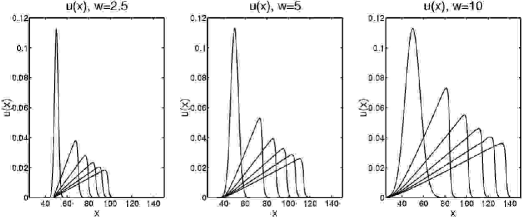
Figure 1: Ramps and cliffs for $b=0$. Inviscid $b$-family, $b=0$, $\alpha=1$, initial width $w=2.5,5,10$.

Figure 1 shows that the ramp and cliff pattern develops in the velocity profile under the peakon equation (1) with $g(x)=e^{-|x|/\alpha}$ for a set of Gaussian initial conditions $(5\sqrt{\pi})^{-1}\exp(-(x-50)^{2}/w)$ of increasing widths $w=2.5,5,10$, for $\alpha=1$ and $b=0$. Apparently, the ramp solution is numerically stable, but the coexisting peakon solution is not stable in this case. A complete stability analysis of these various solutions is outside the scope of the present paper. Instead we shall investigate the solutions of equation (1) by numerically integrating selected examples.

3.2 Case $b\neq 0$

For $b\neq 0$, the conservation law (12) for traveling waves becomes,

$$\Big{(}(u-c)m^{1/b}\Big{)}\,^{\prime}=0\,,$$ (35)

which yields after one integration

$$(u-c)^{b}m=K\,,$$ (36)

where $K$ is the first integral. For $g(x)=e^{-|x|/\alpha}$, so that $m=u-\alpha^{2}u_{xx}$, this becomes

$$(u-c)^{b}(u-\alpha^{2}u\,^{\prime\prime})=K\,.$$ (37)

For $u-c\neq 0$ we rewrite this as

$$\alpha^{2}u\,^{\prime\prime}=u-K(u-c)^{-b}\,$$ (38)

and integrate again to give the second integral in two separate cases,

$$\alpha^{2}{u\,^{\prime}\,}^{2}=\left\{\begin{array}[]{l}u^{2}-\frac{2K}{1-b}(u-c)^{1-b}+2H\quad\hbox{for}\quad b\neq 1\,,\par\\[4.0pt] u^{2}-2K\log(u-c)+2H\quad\hbox{for}\quad b=1\,.\par\end{array}\right.$$

We shall rearrange this into quadratures:

$$\pm\,\frac{dz}{\alpha}=\frac{du}{\Big{[}u^{2}-\frac{2K}{1-b}(u-c)^{1-b}+2H\Big{]}^{1/2}}\quad\hbox{for}\quad b\neq 1\,,$$ (40)

and

$$\pm\,\frac{dz}{\alpha}=\frac{du}{\Big{[}u^{2}-2K\log(u-c)+2H\Big{]}^{1/2}}\quad\hbox{for}\quad b=1\,.$$ (41)

For $b=1$ and $K\neq 0$, the integral in equation (41) is transcendental.

3.2.1 Special cases of traveling waves for $b\neq 0$

• For $K=0$ the two quadratures (40) and (41) are equal, independent of $b$, and elementary, thereby yielding the traveling wave solutions

  $$e^{-|z|/\alpha}=\frac{u+\sqrt{u^{2}+2H}}{c+\sqrt{c^{2}+2H}}\,,$$ (42)

  with $u-c=0$ at $z=0$.

• For $H=0$ equation (42) recovers the peakon traveling wave.

• For $H>0$ equation (42) gives a rightward moving traveling wave that is a continuous deformation of the peakon.

• For $H>0$ and $c=0$ equation (42) gives stationary solutions of the

  form

  $$u+\sqrt{u^{2}+2H}\simeq e^{-|z|/\alpha}\,.$$ (43)

3.3 Case $b>0$

3.3.1 Pulsons for $b>0$

Equation (1) for $b>0$ has nontrivial solutions vanishing as $|z|\to\infty$ that allow $K=0$ in equation (36), so that

$$(u-c)^{b}m=0\,.$$ (44)

This admits the generalized function solutions

$$m=c\delta(z)\quad\hbox{and}\quad u=g*m=cg(z)\,,$$ (45)

matched by $u-c=0$ at $z=0$. This is the pulson traveling wave, whose shape in $u$ is given by the kernel $g$. The constant velocity case $u=c$ is a trivial traveling wave.

Remark 3.6 (Pulson and peakon traveling waves)

The pulson solution (45) requires $g(0)=1$ and $g\,^{\prime}(0)=0$. We shall assume for definiteness that the even function $g(z)$ achieves its maximum at $g(0)=1$, so that the symmetric pulson traveling wave $u(x,t)=cg(x-ct)$ moves at the speed of its maximum, which occurs at its center of symmetry. For example, the peakon $u(x,t)=ce^{-|x-ct|}$ moves at the speed of its peak.

3.3.2 Peakons for $b>1$

Equation (37), for which $g(x)=e^{-|x|/\alpha}$, yields the peakon traveling wave

$$u(z)=ce^{-|z|/\alpha}\quad\hbox{and}\quad m(z)=u-\alpha^{2}u\,^{\prime\prime}=2c\delta(z/\alpha)\,$$ (46)

when $K=0$.

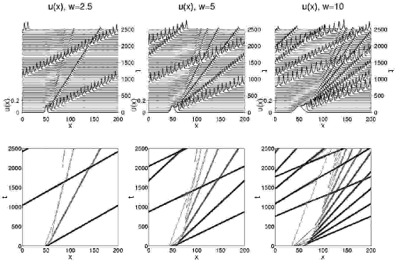
Figure 2: Peakons for $b=2$. Inviscid $b$-family, $b=2$, $\alpha=1$, initial width $w=2.5,5,10$.

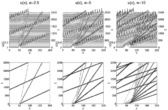
Figure 3: Peakons for $b=3$. Inviscid $b$-family, $b=3$, $\alpha=1$, initial width $w=2.5,5,10$.

Figures 2 and 3 show the effects of varying the width $w$ of a Gaussian initial condition $(5\sqrt{\pi})^{-1}\exp(-(x-50)^{2}/w)$ for the peakon equation in a periodic domain, when $\alpha=1$ and $b=2,3$. As the width of the initial Gaussian increases, the figures show that more peakons of width $\alpha=1$ are emitted. (This is consistent with conservation of momentum.) The peakons are observed to be stable for $b>1$, they propagate as solitary traveling waves, and they interact elastically. We shall discuss the peakon interactions in more detail in sections 5 through 8.

3.4 Case $b<0$

We shall examine the cases $b=-0.5,-1,-2,-3,-4$. Numerical results for $b=-2$ and $b=-3$ are described in section 3.4.6. For other values of $b<0$ the analysis is similar, but it involves less elementary considerations such as transcendental or hyperelliptic functions. The numerics shown later will demonstrate that the elementary solutions discussed here, many of them stationary, do tend to emerge in numerical integrations of the initial value problem for equation (1) with $b\leq-1$.

3.4.1 Case $b=-1/2$

Figure 4 shows that a ramp and cliff pattern develops in the velocity profile under the peakon equation (1) with $g(x)=e^{-|x|/\alpha}$ for a set of Gaussian initial conditions $(5\sqrt{\pi})^{-1}\exp(-(x-100)^{2}/w)$ of increasing width $w=10,15,20$, for $\alpha=1$ and $b=-1/2$. Apparently, the ramp solution is numerically stable for $b=-1/2$.

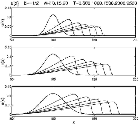
Figure 4: Ramps and cliffs for $b=-1/2$. Inviscid $b$-family, $b=-1/2$, $\alpha=1$, initial width $w=10,15,20$.

3.4.2 Case $b=-1$

For $b=-1$, equation (40) becomes

$$\pm\,\frac{dz}{\alpha}=\frac{du}{\Big{[}u^{2}-K(u-c)^{2}+2H\Big{]}^{1/2}}\,,$$ (47)

which integrates to

$$e^{-|z|/\alpha}=\frac{u+\sqrt{u^{2}-K(u-c)^{2}+2H}+Kc}{c+\sqrt{c^{2}+2H}+Kc}\,,$$ (48)

with $u-c=0$ at $z=0$. ($K=0$ and $H=0$ recovers the peakon traveling wave.)

Remark 3.7 (Stationary plane wave solutions for $b=-1$)

Equation (1) for $b=-1$ is satisfied for any wavenumber $k$ by,

$$m=\cos(k(x-ct)+\phi_{0})\quad\hbox{and}\quad u=\hat{g}(k)\cos(k(x-ct)+\phi_{0})\,,$$ (49)

where $\hat{g}(k)$ is the Fourier transform of the kernel $g(x)$ and $\phi_{0}$ is a constant phase shift. In the absence of linear dispersion, these solutions are stationary, $c=0$. When linear dispersion is added to equation (1), these solutions are the 1D analogs of Rossby waves in the 2D quasigeostrophic equations.

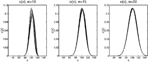
Figure 5: Stationary solutions for $b=-1$. Inviscid $b$-family, $b=-1$, $\alpha=1$, initial width $w=10,15,20$.

Figure 5 shows the velocity profiles under evolution by the peakon equation, (1) with $g(x)=e^{-|x|/\alpha}$, for a set of Gaussian initial conditions of increasing width $w=10,15,20$ for $\alpha=1$ and $b=-1$. Evidently, the coexisting peakon solution for $b=-1$ does not emerge because $K\neq 0$ and $H\neq 0$ for this initial condition. Instead, the stable solution is essentially stationary with a slight rightward drift and leaning slightly to the right. The reason for this lethargic propagation becomes clear upon writing the b-equation solely in terms of the velocity $u(x,t)$ as

$$u_{t}+(b+1)uu_{x} = \alpha^{2}(u_{xxt}+uu_{xxx}+bu_{x}u_{xx})$$

$$= \alpha^{2}\partial_{x}\Big{(}u_{xt}+uu_{xx}+\frac{b-1}{2}u_{x}^{2}\Big{)}$$

$$= \alpha^{2}\partial_{x}^{2}\Big{(}u_{t}+uu_{x}+\frac{b-3}{2}u_{x}^{2}\Big{)}\,.$$

Remark 3.8 ($b=-1$ is a turning point)

When $b=-1$ the nonlinear steepening term $(b+1)uu_{x}$ vanishes in (3.4.2) and the residual propagation is due to its nonlinear “curvature terms” with higher order derivatives. In the parameter regime $b>-1$ (resp. $b<-1$) the solutions of equation (1) or (3.4.2) move rightward (resp. leftward), provided the curvature terms on the right hand side of equation (3.4.2) are either negative, or sufficiently small.

Remark 3.9 (Short wave limit equation)

The high wavenumber, or short wave, limit of equation (3.4.2) is

$$\partial_{x}^{2}\Big{(}u_{t}+uu_{x}+\frac{b-3}{2}u_{x}^{2}\Big{)}=0\,.$$ (51)

For $b=2$ and $\lim_{x\to-\infty}u_{x}=0$, this integrates to become the Hunter-Saxton equation [12]. For $b=3$, it is the second derivative of the Burgers equation.

3.4.3 Case $b=-2$ stationary solutions

For $b=-2$, the traveling wave quadrature (40) becomes an elliptic integral

$$\pm\,\frac{dz}{\alpha}=\frac{d(u-c)}{\Big{[}u^{2}-\frac{2K}{3}(u-c)^{3}+2H\Big{]}^{1/2}}\,.$$ (52)

The hyperbolic limit of this equation for $H=0$ vanishes at infinity for the stationary solution ($c=0$) to give

$$u(z)=\frac{3}{2K}{\rm sech}^{2}\frac{z}{2\alpha}\,.$$ (53)

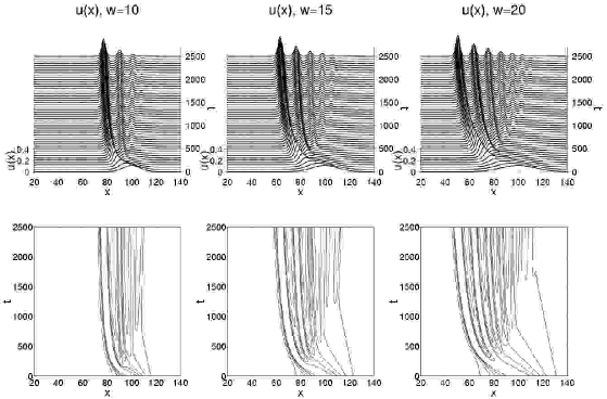
Figure 6: Stationary solutions for $b=-2$. Inviscid $b$-family, $b=-2$, $\alpha=1$, initial width $w=10,15,20$.

3.4.4 Case $b=-3$ stationary solutions

For $b=-3$, the hyperbolic limit $H=0$ of equation (40) is

$$\pm\,\frac{dz}{\alpha}=\frac{du}{\Big{[}u^{2}-\frac{K}{2}(u-c)^{4}\Big{]}^{1/2}}\,,$$ (54)

which for $c=0$ is

$$\pm\,\frac{dz}{\alpha}=\frac{du}{u\Big{[}1-\frac{K}{2}u^{2}\Big{]}^{1/2}}\,,$$ (55)

and may be integrated in closed form to obtain a continuous deformation of the peakon,

$$\frac{e^{-|z|/\alpha}}{1+\sqrt{1-K/2}}=\frac{u}{1+\sqrt{1-Ku^{2}/2}}\,,\ \hbox{for}\ b=-3\,,\ c=0\hbox{ and }H=0.$$ (56)

Rearranging equation (56) and scaling $u$ by $u_{0}$ gives,

$$u(z)=\frac{u_{0}}{\frac{A}{2}e^{|z|/\alpha}+(1-\frac{A}{2})e^{-|z|/\alpha}}\,,$$ (57)

with $A=1+\sqrt{1-K/2}$, so that $A\in[1,2]$ for $K\in[0,2]$. For $A=1$, we have $u(z)=u_{0}\,{\rm sech}\,(z/\alpha)$. And for $A=2$, we recover the stationary peakon, $u(z)=u_{0}\,e^{-|z|/\alpha}$.

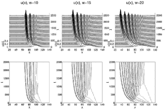
Figure 7: Stationary solutions for $b=-3$. Inviscid $b$-family, $b=-3$, $\alpha=1$, initial width $w=10,15,20$.

3.4.5 Case $b=-4$ stationary solutions

For $b\leq-4$ the analytical expressions for the cnoidal waves become less elementary, because the integral in equation (40) is then hyperelliptic. However, our numerics show that the dynamical behavior for $b=-4$ is similar to that of the cases $b=-2$ and $b=-3$ shown in Figures 6-7. Namely, a series of transient leftward propagating pulses, or leftons, of width alpha emerge and tend to a nearly steady state. Consistent with momentum (area) conservation and the tendency toward pulses of width alpha, the number of emerging leftons increases with the width of the initial Gaussian. At a longer time scale, this train of pulses appears to tend toward stationary ($c\to 0$).

3.4.6 Numerical Results for $b=-2$ and $b=-3$

Figures 6 and 7 show that a series of leftons in the velocity profile emerges under the peakon equation for a set of Gaussian initial conditions of increasing width $w=10,15,20$, for $\alpha=1$ and $b=-2,-3$. Apparently these are not peakons, because the velocity at which they move is not equal to their height. The leftons emerge from the initial Gaussian in order of height and then tend toward a nearly stationary state. The number of emerging pulses increases with the width of the initial Gaussian, as expected from momentum (area) conservation and the tendency toward pulses of width alpha, and the leftward speed of the emerging pulses increases with the magnitude of $b$. The latter is consistent with the coefficient $(b+1)$ of the nonlinearity in equation (3.4.2) as $b$ becomes more negative.

Figure 8 shows the leftons at time $T=2500$, versus $u(x)\simeq{\rm sech}^{2}(x/(2\alpha))$ for $b=-2$, and versus $u(x)\simeq{\rm sech}(x/\alpha)$ for $b=-3$. By this time, the leftons have become stationary solutions with $c=0$ for both $b=-2$ and $b=-3$.

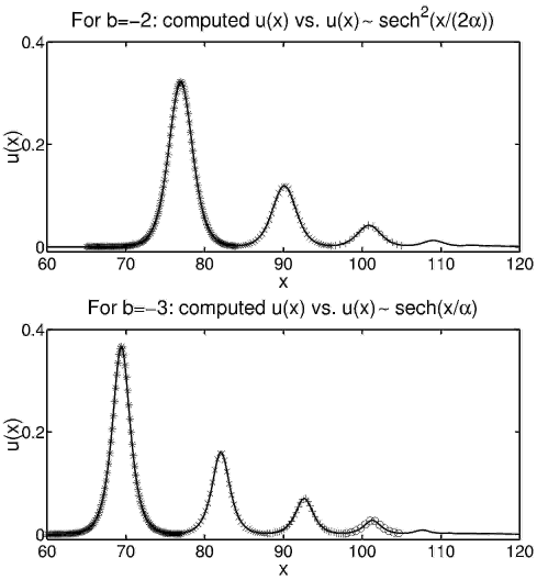
Figure 8: Stationary solutions for $b=-2$ versus $u(x)\simeq{\rm sech}^{2}(x/(2\alpha))$, and for $b=-3$ versus $u(x)\simeq{\rm sech}(x/\alpha)$. Inviscid $b$-family, $b=-2,-3$, $\alpha=1$, initial width $w=10$.

4 Pulson interactions for $b>0$

As we have seen in section 3.3.1, the b-family of equations (1) admits the pulson traveling wave solution (45) for $b>0$. The interaction dynamics among $N$ of these pulsons is obtained by superposing the traveling wave solutions $u(x,t)=cg(x-ct)$ as

$$u(x,t)=\sum_{i=1}^{N}p_{i}(t)g(x-q_{i}(t))\quad\hbox{and}\quad m(x,t)=\sum_{i=1}^{N}p_{i}(t)\delta(x-q_{i}(t))\,,$$ (58)

for any $b>0$ and $u=g*m$, where the function $g$ is even so that $g\,^{\prime}(0)=0$ and bounded and we may set $g(0)=1$. For these superpositions of pulsons to be exact solutions, the time dependent parameters $p_{i}(t)$ and $q_{i}(t)$ must satisfy the following $N-$dimensional particle dynamics equations obtained by substituting (58) into equation (1),

$$\dot{p}_{i} = (1-b)\,p_{i}\sum_{j=1}^{N}p_{j}\,g\,^{\prime}(q_{i}-q_{j})=(1-b)\,\frac{\partial G_{N}}{\partial q_{i}}\,,$$ (59)

$$\dot{q}_{i} = \sum_{j=1}^{N}p_{j}\,g(q_{i}-q_{j})=\frac{\partial G_{N}}{\partial p_{i}}\,.$$ (60)

Here the generating function $G_{N}$ is obtained by restricting the norm $\|m\|_{g}^{2}$ in (29) to the class of superposed traveling wave solutions (58), as

$$G_{N}=\frac{1}{2}\sum_{i,j=1}^{N}p_{i}p_{j}\,g(q_{i}-q_{j})\,.$$ (61)

Thus, the symmetric kernel $g(x)$ determines the shape of the traveling wave solutions (58), and these traveling waves interact nonlinearly via the pulson dynamics of $p_{i}(t)$ and $q_{i}(t)$ with $i=1,\dots,N$ in equations (59) and (60) for $b>0$. We shall see that the character of these interactions depends vitally on the value of $b$.

4.1 Pulson interactions for $b=2$

When $b=2$, equations (59) and (60) describe the canonical dynamics of a Hamiltonian system with $N$ degrees of freedom. These are the geodesic pulson equations studied in Fringer and Holm [7], in which the following results are obtained,

$\bullet$ Equation (1) conserves the kinetic energy $\frac{1}{2}\|m\|_{g}^{2}=\frac{1}{2}\int_{-\infty}^{\infty}m\,g*m\,dx$.

$\bullet$ Equations (59) and (60) describe canonical geodesic motion in an $N-$dimensional configuration space whose co-metric is $g^{ij}(q)=g(q_{i}-q_{j})$.

$\bullet$ The generating function $G_{N}$ is the kinetic energy Hamiltonian for the canonical geodesic motion.

$\bullet$ The solutions in (58) behave as particle-like pulses whose pairwise interactions as determined by equations (59) and (60) comprise nonlinear, but elastic, scattering events.

$\bullet$ The pairwise interactions for the pulsons can be solved analytically for any symmetric function $g(x)$.

Remark 4.1

As we shall show, the last two statements also hold for any $b>1$.

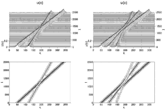
Figure 9: Peakons of width $\alpha$ for $b=2$: collisions. Inviscid $b$-family, $b=2$, $\alpha=5$, initial width $w=5$.

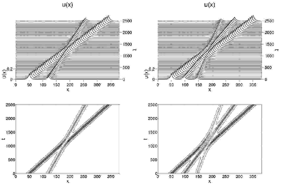
Figure 10: Peakons of width $\alpha$ for $b=3$: collisions. Inviscid $b$-family, $b=3$, $\alpha=5$, initial width $w=5$.

4.2 Peakon interactions for $b=2$ and $b=3$: numerical results

• Figure 9 shows the evolution of the velocity profiles in the 2-peakon and 3-peakon interactions for $b=2$, with $g(x)=e^{-|x|/\alpha}$ and a periodic domain. The 3-peakon interaction decomposes into a series of 2-peakon interactions. These simulations verify the analytical results for the 2-peakon interaction to three significant figures over propagation distances of about sixty peakon widths.

• Figure 10 shows the evolution of the velocity profiles in the 2-peakon and 3-peakon interactions for $b=3$, with $g(x)=e^{-|x|/\alpha}$ and a periodic domain.

  

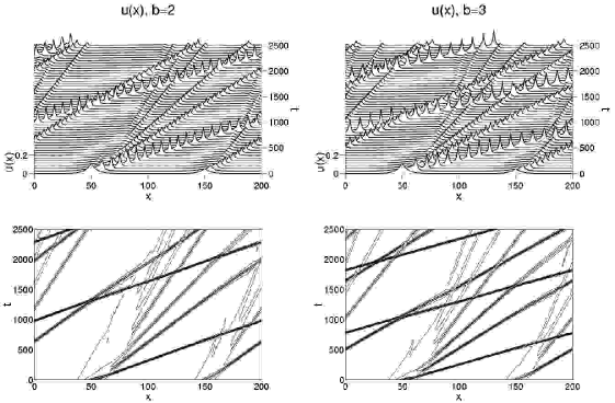
  Figure 11: Peakons of width $>\alpha$ for $b=2,3$: emergence of width-$\alpha$ peakons. Inviscid $b$-family, $b=2,3$, $\alpha=1$, initial width $w=5$.

• Figure 11 shows that peakons of initial width greater than $\alpha$ break up into peakons of width $\alpha$ under the evolution of the peakon equation in a periodic domain at fixed values of $\alpha=1$ and $b=2,3$. The emitted peakons are stable, propagate as solitary traveling waves, and interact elastically. Conversely, a peakon or other initial condition that is narrower than $\alpha$ will decompose into two oppositely moving trains of peakons and antipeakons, each of width $\alpha$.

4.3 Pulson-Pulson interactions for $b>0$ and symmetric $g$

For $N=2$, the pulson dynamics in equations (59) and (60) for $b>0$ reduces to

$$\frac{dp_{1}}{dt}=(1-b)\frac{\partial G}{\partial q_{1}}\,,\quad\frac{dp_{2}}{dt}=(1-b)\frac{\partial G}{\partial q_{2}},$$ (62)

$$\frac{dq_{1}}{dt}=\frac{\partial G}{\partial p_{1}},\quad\frac{dq_{2}}{dt}=\frac{\partial G}{\partial p_{2}},$$ (63)

and the generating function from (61) is given by

$$G=\frac{1}{2}(p_{1}^{2}+p_{2}^{2})+p_{1}p_{2}\,g(q_{1}-q_{2})\,.$$ (64)

(This is the Hamiltonian and the equations are canonical only for $b=2$, which includes the Camassa-Holm case for which $g(q_{1}-q_{2})=e^{-|q_{1}-q_{2}|}$ gives the peakon solutions.)

Conservation laws and reduction to quadrature

Besides the total momentum

$$P=p_{1}+p_{2}\,,$$ (65)

the two-pulson system for $b>0$ and symmetric $g$ also conserves a second quantity that is quadratic in $p_{1}$ and $p_{2}$, namely

$$H=p_{1}p_{2}\big{(}1-g(q_{1}-q_{2})\big{)}^{b-1}\,.$$ (66)

For a Hamiltonian system with two degrees of freedom this second conservation law would be enough to ensure integrability, by Liouville’s theorem. Even in the present case of $b>0$ without a Hamiltonian structure, this will be sufficient to reduce the 2-pulson system to quadratures.

Following the analysis for the case $b=2$ and arbitrary $g$ in Fringer and Holm [7], we introduce sum and difference variables as

$$P=p_{1}+p_{2}\,,\quad Q=q_{1}+q_{2}\,,\quad p=p_{1}-p_{2}\,,\quad q=q_{1}-q_{2}\,.$$ (67)

In these variables, the generating function (64) becomes

$$G=\frac{1}{4}P^{2}(1+g(q))+\frac{1}{4}p^{2}(1-g(q))\,,$$ (68)

and the second constant of motion (66) becomes

$$H=\frac{1}{4}(P^{2}-p^{2})\big{(}1-g(q)\big{)}^{b-1}\,.$$ (69)

Likewise, the 2-pulson equations of motion transform to sum and difference variables as

$$\begin{array}[]{l}\frac{dP}{dt}=2(1-b)\frac{\partial G}{\partial Q}=0\,,\cr\frac{dQ}{dt}=2\frac{\partial G}{\partial P}=P(1+g(q))\,,\cr\frac{dp}{dt}=2(1-b)\frac{\partial G}{\partial q}\par=\frac{1}{2}(1-b)(P^{2}-p^{2})g\,^{\prime}(q)\,,\cr\frac{dq}{dt}=2\frac{\partial G}{\partial p}=p(1-g(q)).\end{array}$$

Eliminating $p^{2}$ between the formula for $H$ and the equation of motion for $q$ yields

$$\left(\frac{dq}{dt}\right)^{2}=P^{2}\big{(}1-g(q)\big{)}^{2}-4H\big{(}1-g(q)\big{)}^{3-b}\,.$$ (71)

We rearrange this into the following quadrature,

$$dt=\frac{dg(q)}{g\,^{\prime}(q)\sqrt{Z}},\qquad Z=P^{2}\big{(}1-g(q)\big{)}^{2}-4H\big{(}1-g(q)\big{)}^{3-b}\,.$$ (72)

This simplifies to the quadratic $Z=P^{2}\big{(}1-g(q)\big{)}^{2}-4H$ when $b=3$. For the peakon case, we have $g(q)=e^{q}$ so that $g\,^{\prime}(q)=g(q)$ and the quadrature (72) simplifies to an elementary integral for $b=-1,0,1,2,3$. Having obtained $q(t)$ from the quadrature, the momentum difference $p(t)$ is found from (69) via the algebraic expression

$$p^{2}=P^{2}-\frac{4H}{\big{(}1-g(q)\big{)}^{b-1}}\,,$$ (73)

in terms of $q$ and the constants of motion $P$ and $H$. Finally, the sum $Q(t)$ is found by a further quadrature. The remainder of the solution for arbitrary $b$ and $g$ closely follows Fringer and Holm [7] for the case $b=2$.

Upon writing the quantities $H$, $P$ and $G$ as

$$H=c_{1}c_{2},\quad P=c_{1}+c_{2},\quad G=\frac{1}{2}c_{1}^{2}+\frac{1}{2}c_{2}^{2}=\frac{1}{2}P^{2}-H\,,$$ (74)

in terms of the asymptotic speeds of the pulsons, $c_{1}$ and $c_{2}$, we find the relative momentum relation,

$$p^{2}=(c_{1}+c_{2})^{2}-\frac{4c_{1}c_{2}}{\big{(}1-g(q)\big{)}^{b-1}}\,.$$ (75)

This equation has several implications for the qualitative properties of the 2-pulson collisions.

Definition 4.2

Overtaking, or rear-end, pulson collisions satisfy $c_{1}c_{2}>0$, while head-on pulson collisions satisfy $c_{1}c_{2}<0$.

The pulson order $q_{1}<q_{2}$ is preserved in an overtaking, or rear-end, collision when $b>1$. This follows, as

Proposition 4.3 (Preservation of pulson order)

For overtaking, or rear-end, collisions when $b>1$, the 2-pulson dynamics preserves the sign condition $q=q_{1}-q_{2}<0$.

Proof.

Suppose the peaks were to overlap in a collision for $b>1$, thereby producing $q=0$ during a collision. The condition $g(0)=1$ implies the second term in (75) diverges for $b>1$ when the overlap occurs. However, this divergence would contradict $p^{2}\geq 0$. $\Box$

Consequently, seen as a collision between two initially well-separated “particles” with initial speeds $c_{1}$ and $c_{2}$, the separation $q(t)$ reaches a nonzero distance of closest approach $q_{min}$ in an overtaking, or rear-end, collision that may be expressed in terms of the pulse shape as,

Corollary 4.4 (Minimum separation distance)

The minimum separation distance reachable in two-pulson collisions with $c_{1}c_{2}>0$ is given by,

$$\big{(}1-g(q_{min})\big{)}^{b-1}=\frac{4c_{1}c_{2}}{(c_{1}+c_{2})^{2}}\,.$$ (76)

Proof.

Set $p^{2}=0$ in equation (75). $\Box$

Remark 4.5

We shall use result (76) later in checking the accuracy of our numerical simulations of these two-pulson interactions.

Proposition 4.6 (Head-on collisions admit $q\to 0$)

The 2-pulson dynamics allows the overlap $q\to 0$ when $b>1$ in head-on collisions.

Proof.

Because $p^{2}\geq 0$, the overlap $q\to 0$ implying $g\to 1$ is only possible in equation (75) with $b>1$ for $c_{1}c_{2}<0$. That is, for the head-on collisions. $\Box$

Remarks about head-on collisions.

For $b>1$, equation (75) implies that $p^{2}\to\infty$ diverges when $q\to 0$ in head-on collisions. The case $b=1$ is regular and equation (75) reduces to the constant relation $p^{2}=(c_{1}-c_{2})^{2}$. For $0<b<1$, the quantity $p^{2}$ no longer diverges when $q\to 0$ and the solution for the relative momentum in head-on collisions is again regular.

4.4 Pulson-antiPulson interactions for $b>1$ and symmetric $g$

Head-on Pulson-antiPulson collision.

We consider the special case of completely antisymmetric pulson-antipulson collisions, for which $p_{1}=-p_{2}=p/2$ and $q_{1}=-q_{2}=q/2$ (so that $P=0$ and $Q=0$). In this case, the quadrature formula (72) reduces to

$$\pm(t-t_{0})=\frac{1}{\sqrt{-4H}}\int_{q(t_{0})}^{q(t)}\frac{dq\,^{\prime}}{\big{(}1-g(q\,^{\prime})\big{)}^{(3-b)/2}}\,,$$ (77)

and the second constant of motion in (69) satisfies

$$-4H=p^{2}\big{(}1-g(q)\big{)}^{b-1}\,.$$ (78)

After the collision, the pulson and antipulson separate and travel oppositely apart; so that asymptotically in time $g(q)\to 0$, $p\to 2c$, and $H\to-{c}^{2}$, where $c$ (or $-c$) is the asymptotic speed (and amplitude) of the pulson (or antipulson). Setting $H=-{c}^{2}$ in equation (78) gives a relation for the pulson-antipulson $(p,q)$ phase trajectories for any kernel,

$$p=\pm\,\frac{2c}{\big{(}1-g(q)\big{)}^{(b-1)/2}}\,.$$ (79)

Notice that $p$ diverges for $b>1$ (and switches branches of the square root) when $q\to 0^{+}$, because $g(0)=1$. In contrast, $p$ remains constant for $b=1$ and it vanishes for $b<1$ (and again switches branches of the square root) when $q\to 0^{+}$. Note that our convention for switching branches of the square root allows us to keep $q>0$ throughout, so the particles retain their order.

Remark about preservation of particle identity in collisions.

The relative separation distance $q(t)$ in pulson-antipulson collisions is determined by following a phase point along a level surface of the second constant of motion $H$ in the phase space with coordinates $(q,p)$. Because $H$ is quadratic, the relative momentum $p$ has two branches on such a level surface, as indicated by the $\pm$ sign in equation (79). At the pulson-antipulson collision point, both $q\to 0^{+}$ and either $1/p\to 0^{+}$ or $p\to 0^{+}$, so following a phase point through a collision requires that one choose a convention for which branch of the level surface is taken after the collision. Taking the convention that $p$ changes sign (corresponding to a “bounce”), but $q$ does not change sign (so the “particles” keep their identity) is convenient, because it allows the phase points to be followed more easily through multiple collisions. This choice is also consistent with the pulson-pulson and antipulson-antipulson collisions. In these other “rear end” collisions, as implied by equation (75), the separation distance always remains positive and again the particles retain their identity.

Theorem 4.7 (Pulson-antiPulson exact solution)

The exact analytical solution for the pulson-antipulson collision for any $b$ and any symmetric $g$ may be written as a function of position $x$ and the separation between the pulses $q$ for any pulse shape or kernel $g(x)$ as

$$u(x,q)=\frac{c}{\big{(}1-g(q)\big{)}^{(b-1)/2}}\Big{[}g(x+q/2)-g(x-q/2)\Big{]},$$ (80)

where $c$ is the pulson speed at sufficiently large separation and the dynamics of the separation $q(t)$ is given by the quadrature (77) with $\sqrt{-4H}=2c$.

Proof.

The solution (58) for the velocity $u(x,t)$ in the head-on pulson-antipulson collision may be expressed in this notation as

$$u(x,t)=\frac{p}{2}g(x+q/2)-\frac{p}{2}g(x-q/2)\,.$$ (81)

In using equation (79) to eliminate $p$ this solution becomes equation (80). $\Box$

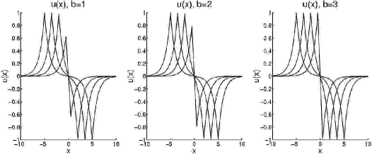
Figure 12: Peakon-antipeakon collisions for $b=1,2,3$. Inviscid $b$-family, $b=1,2,3$, $\alpha=1$, initial width $w=1$.

Figure 12 shows the exact solutions for the Peakon-antiPeakon collision in the cases $b=1$, $b=2$, and $b=3$. The positive and negative peaks approach each other until the solution develops a negative vertical slope in finite time. As the separation $q\to 0$, the positive and negative peaks “bounce,” thereby reversing polarity, after which they separate in opposite directions.

4.5 Specializing Pulsons to Peakons for $b=2$ and $b=3$

We now restrict to $g(x)=e^{-|x|}$, the Green’s function for the 1D Helmholtz operator satisfying

$$\Big{(}1-\frac{d^{2}}{dx^{2}}\Big{)}e^{-|x|}=2\delta(x)\,.$$ (82)

In this case, $m=u-\alpha^{2}u_{xx}$, the pulson traveling wave solution is given by $u(x,t)=cg(x-ct)=ce^{-|x-ct|}$, has a discontinuity in derivative at its peak, and is called the peakon. For $b=2$ and $b=3$ in the peakon case the main results are,

• For $b=2$ and $g(x)=e^{-|x|}$, equation (1) becomes the zero-dispersion limit of the integrable Camassa-Holm equation for shallow water waves discovered in Camassa and Holm [2]. Upon restoring its linear dispersion, this equation was recently proved to be a higher-order accurate asymptotic description of shallow water waves in Dullin et al. [6].

• For $b=3$ and $g(x)=e^{-|x|}$, equation (1) becomes the integrable partial differential equation studied in Degasperis, Holm and Hone [4].

• When $g(x)=e^{-|x|}$ the $N-$peakon dynamics for both $b=2$ and $b=3$ turns out to be integrable – as is the dynamics of the original PDE (1). The solutions of the initial value problem for (1) for both $b=2$ and $b=3$ may be found analytically by using the Isospectral Scattering Transform (IST) method.

• The two cases $b=2$ and $b=3$ have quite different isospectral eigenvalue problems. These are discussed in Camassa and Holm [2] and in Dullin et al. [6] for the case $b=2$, and in Degasperis, Holm and Hone [4] for the case $b=3$. See also Beals, Sattinger and Smigialski [1] for a discussion of solving the inverse isospectral problem using classical methods for the case $b=2$.

5 Peakons of width $\alpha$ for arbitrary $b$

When $g=e^{-|x|/\alpha}$, we may invert the velocity-momentum relation $u=g*m$ by using the Green’s function expression (82) with the Helmholtz operator to find $m=u-\alpha^{2}u_{xx}$. Hence, equation (1) may be rearranged into the local momentum conservation law,

$$m_{t}=-\,\frac{\partial}{\partial x}\Big{(}mu+\frac{b-1}{2}u^{2}-\frac{b-1}{2}\alpha^{2}u_{x}^{2}\Big{)}\,.$$ (83)

This conservation law for peakons may also be rewritten in convection form:

$$u_{t}+uu_{x}=-\,\tau_{x}\quad\hbox{with}\quad(1-\alpha^{2}\partial_{x}^{2})\tau=\frac{b}{2}u^{2}+\frac{3-b}{2}\alpha^{2}u_{x}^{2}\,.$$ (84)

The two forms (83) and (84) of the b-family of equations (1) suggest that values $b=0,1,3$ are special. These values of $b$ are natural candidates for boundaries, or bifurcation points for changes in solution behavior.

Equation (84) describes peakons of shape $g(x)=e^{-|x|/\alpha}$. This peakon equation will form the basis of the rest of our study.

5.1 Slope dynamics for Peakons: inflection points and the steepening lemma when $1<b\leq 3$

We shall consider solution dynamics of equation (84) in the peakon case satisfying (46), or equivalently, equation (1) with $g(x)=e^{-|x|/\alpha}$, which satisfies

$$(1-\alpha^{2}\partial_{x}^{2})e^{-|x|/\alpha}=2\alpha\delta(x)\,.$$ (85)

For this case, and with vanishing boundary conditions at spatial infinity, equations (84) and (85) imply the peakon equation on the real line,

$$u_{t}+uu_{x}=-\,\frac{1}{2\alpha}\int_{-\infty}^{\infty}e^{-|x-y\,|/\alpha}\Big{(}buu_{y}+(3-b)\alpha^{2}u_{y}u_{yy}\Big{)}\,dy\,.$$ (86)

Taking the $x-$derivative gives the equation for the slope $u_{x}(x,t)$

$$u_{xt}+uu_{xx}+u_{x}^{2} = -\,\frac{1}{2\alpha}\frac{\partial}{\partial x}\int_{-\infty}^{\infty}e^{-|x-y\,|/\alpha}\Big{(}buu_{y}+(3-b)\alpha^{2}u_{y}u_{yy}\Big{)}\,dy$$ (87)

$$=\frac{1}{2\alpha^{2}}\int_{-\infty}^{\infty}e^{-|x-y\,|/\alpha}\,{\rm sgn}\,(x-y)\Big{(}buu_{y}+(3-b)\alpha^{2}u_{y}u_{yy}\Big{)}\,dy\,.$$

We shall use these expressions to prove the following.

Proposition 5.1 (Peakon Steepening Lemma)

For $b$ in the range $1<b\leq 3$ a sufficiently negative slope at an inflection point of $u$ will become vertical in finite time under the dynamics of the peakon equation (86).

Proof.

Following Camassa and Holm [2], we shall consider the evolution of the slope $u_{x}$ at an inflection point $x=\bar{x}(t)$. Define the slope at the inflection point as $s(t)=u_{x}(\bar{x}(t),t)$ and note that $u_{xx}(\bar{x}(t),t)=0$. Then equation (87) yields the following evolution equation for $s(t)$

$$\frac{ds}{dt}+s^{2}=\frac{1}{2\alpha^{2}}\int_{-\infty}^{\infty}\!\!\!\!\!e^{-|\,\bar{x}(t)-y\,|/\alpha}\,{\rm sgn}\,(\bar{x}(t)-y)\frac{1}{2}\frac{\partial}{\partial y}\Big{(}bu^{2}+(3-b)\alpha^{2}u_{y}^{2}\Big{)}\,dy$$ (88)

Integrating by parts using the definition $|y|=y\,{\rm sgn}\,(y)$, so that $d|y|/dy=\,{\rm sgn}\,(y)+2y\delta(y)$, and recalling that $y\delta(y)=0$, gives

$$\frac{ds}{dt}=-\,\Big{(}\frac{b-1}{2}\Big{)}s^{2}+\frac{b}{2\alpha^{2}}\,u^{2}-\frac{1}{2\alpha^{2}}\int_{-\infty}^{\infty}\!\!\!\!\!e^{-|\,\bar{x}(t)-y\,|/\alpha}\frac{1}{2\alpha}\Big{(}bu^{2}+(3-b)\alpha^{2}u_{y}^{2}\Big{)}\,dy$$

Hence, in the range $0\leq b\leq 3$ the last term is negative and we have the slope inequality,

$$\frac{ds}{dt}\leq-\,\Big{(}\frac{b-1}{2}\Big{)}s^{2}+\frac{b}{2\alpha^{2}}\,u^{2}\quad\hbox{for}\quad 0\leq b\leq 3\,.$$ (89)

We suppose the solution satisfies $(bu^{2}/\alpha^{2})<M$ for some constant $M$. Then,

$$\frac{ds}{dt}\leq-\,\Big{(}\frac{b-1}{2}\Big{)}s^{2}+\frac{M}{2}\quad\hbox{for}\quad 0\leq b\leq 3\,.$$ (90)

Consequently, if $b>1$,

$$\frac{dX}{1-X^{2}}=d\,{\rm coth}^{-1}(X)\leq\sqrt{M}\quad\hbox{for}\quad X=\sqrt{\frac{b-1}{M}}\,s\,.$$ (91)

This implies, for $s\leq-\sqrt{M}$ initially negative, that

$$s\leq\sqrt{M}\,{\rm coth}\Big{(}\sigma+\sqrt{\frac{b-1}{M}}\frac{M}{2}\,t\Big{)}\quad\hbox{for}\quad 1<b\leq 3\,,$$ (92)

where the dimensionless integration constant $\sigma<0$ determines the initial slope, which is negative. Under these circumstances, the slope at the inflection point must become vertical by time $t=-2\sigma/\sqrt{M(b-1)}$.

$\Box$

Remarks for $1<b\leq 3$.

• If the initial condition is antisymmetric, for $1<b\leq 3$, then the inflection point at $u=0$ is fixed and $d\bar{x}/dt=0$, due to the mirror reflection symmetry $(u,x)\rightarrow(-u,-x)$ admitted by equation (86). In this case, $M=0$ and equation (90) implies

  $$ds/dt\leq-\,\Big{(}\frac{b-1}{2}\Big{)}s^{2}\quad\Rightarrow\quad s(t)\leq\frac{-2}{b-1}\Big{(}\frac{1}{t_{0}-t}\Big{)}\,,$$ (93)

  so verticality $s=-\infty$ will develop in finite time, regardless of how small the initial slope $|s(0)|$, provided it is negative, $s(0)<0$, as in figure 12. If the initial slope is positive, then under this evolution it will relax to zero from above.

• Consequently, traveling wave solutions of (86) cannot have the usual sech-like shape for solitons because inflection points with sufficiently negative slope can produce unsteady changes in the shape of the solution profile.

5.2 Cases $0\leq{b}\leq 1$

In the range $0\leq{b}\leq 1$, we have from (19) that

$$\int_{-\infty}^{\infty}|m|^{1/b}\,dx=\int_{-\infty}^{\infty}|m_{0}|^{1/b}\,dx\,,\quad\hbox{where}\quad m_{0}(x)=m(x,0)\,.$$ (94)

This conservation law implies an elliptic regularity estimate showing that the slope $s=u_{x}$ is always bounded under the dynamics of the peakon equation (86). See Holm and Titi [2002] for a proof of this result and more discussion of its implications.

6 Adding viscosity to peakon dynamics

In the remainder of this paper, we shall restrict our attention to the peakon case $g(x)=e^{-|x|/\alpha}$ with length scale $\alpha$, and investigate the fate of the peakon solutions when viscosity is introduced for given values of $b$ and $\alpha$. For purposes of comparison with previous results in the literature, we shall also extend equation (1) to a new family of equations that includes the Burgers equation by introducing two additional real parameters. These are the viscosity $\nu$ and a multiplier $\beta$ for the stress, or pressure gradient.

First, we shall introduce constant viscosity $\nu>0$ into (1) to form the viscous b-family of equations for the peakon case $g(x)=e^{-|x|/\alpha}$, as follows,

$$m_{t}\ +\ \underbrace{\ \ um_{x}\ \ }_{\hbox{convection}}\ +\ \underbrace{\ \ b\,u_{x}m\ \ }_{\hbox{stretching}}\ =\ \underbrace{\ \ \nu\,m_{xx}\ }_{\hbox{viscosity}}\,,\quad\hbox{with}\quad m=u-\alpha^{2}u_{xx}\,.$$ (95)

As in equation (3.4.2), this equation with viscosity may be expressed solely in terms of the velocity $u(x,t)$ as

$$u_{t}+(b+1)uu_{x}-\nu u_{xx} = \alpha^{2}(u_{xxt}+uu_{xxx}+bu_{x}u_{xx}-\nu u_{xxxx})$$

$$= \alpha^{2}\partial_{x}\Big{(}u_{xt}+uu_{xx}-\nu u_{xxx}+\frac{b-1}{2}u_{x}^{2}\Big{)}$$

$$= \alpha^{2}\partial_{x}^{2}\Big{(}u_{t}+uu_{x}-\nu u_{xx}+\frac{b-3}{2}u_{x}^{2}\Big{)}\,.$$

Thus, the nonlinear steepening term increases with $b$ as $(b+1)uu_{x}$. When $\alpha\to 0$ the previous equation reduces to

$$u_{t}+(b+1)uu_{x}-\nu u_{xx}=0\,,$$ (97)

and one then recovers the usual Burgers equation either by rescaling dimensions, or by setting $b=0$. For $b=2$, equation (95) is the one-dimensional version of the three-dimensional Navier-Stokes-alpha model for turbulence [3].

The viscous b-family of peakon equations (95) may be rearranged into two other equivalent forms that are convenient for making the second extension of a stress multiplier. These are either its equivalent conservative form,

$$m_{t}=-\,\frac{\partial}{\partial x}\Big{(}mu+\frac{b-1}{2}u^{2}-\frac{b-1}{2}\alpha^{2}u_{x}^{2}\Big{)}+\nu\,m_{xx}\,,$$ (98)

or its equivalent convective form,

$$(1-\alpha^{2}\partial_{x}^{2})\big{(}u_{t}+uu_{x}-\nu u_{xx}\big{)}=-\,\partial_{x}\Big{(}\frac{b}{2}u^{2}+\frac{3-b}{2}\alpha^{2}u_{x}^{2}\Big{)}\,.$$ (99)

Stress multiplier $\beta$.

Next, we shall introduce a stress multiplier $\beta$ as a second parameter that for $\beta\neq 1$ deforms the convective form of the viscous b-family of equations (99) into the following family of Burgers-like equations with four parameters $b$, $\alpha$, $\nu$ and $\beta$,

$$u_{t}+uu_{x}-\nu u_{xx}=-\,\beta\,\tau_{x}\quad\hbox{with}\quad(1-\alpha^{2}\partial_{x}^{2})\tau=\frac{b}{2}u^{2}+\frac{3-b}{2}\alpha^{2}u_{x}^{2}\,.$$ (100)

When $\beta=0$, the Burgers$-\alpha\beta$ equation (100) recovers the usual Burgers equation. When $\beta=1$, equation (100) recovers the viscous b-family of peakon equations (95).

We shall seek solutions of the Burgers$-\alpha\beta$ equation (100), either on the real line and vanishing at spatial infinity, or in a periodic domain, for various values of its four parameters $b$, $\alpha$, $\nu$ and $\beta$. Under these boundary conditions, when $\beta\to 1$, equation (100) recovers the convective form (99) of the viscous b-family for peakons with $g(x)=e^{-|x|/\alpha}$. Thus, the viscous b-family of equations (95-99) deforms into the Burgers$-\alpha\beta$ equation (100) when $\beta\neq 1$ and the Burgers$-\alpha\beta$ equation (100) reduces to the usual Burgers equation when $\beta=0$. We shall be interested in the effects of the four parameters $b$, $\alpha$, $\nu$ and $\beta$ on the solutions of the Burgers$-\alpha\beta$ equation (100). We shall be interested especially in the fate of the peakon solutions upon introducing the parameters $\nu$ and $\beta$ so as to retain $H_{\alpha}^{1}$ control of the velocity. As we shall see, such control requires a special relation between the parameters $b$ and $\beta$, namely, $(3-b)\beta=1$.

6.1 Burgers$-\alpha\beta$ equation: analytical estimates

Proposition 6.1 ($H_{\alpha}^{1}$ control of the velocity)

The Burgers$-\alpha\beta$ equation (100) controls the $\alpha-$weighted $H^{1}$ norm of the velocity,

$$\|u\|_{H^{1}_{\alpha}}^{2}=\int_{-\infty}^{\infty}\!\!\big{(}u^{2}+\alpha^{2}u_{x}^{2}\big{)}\,dx$$

for $\alpha^{2}\neq 0$, provided $(3-b)\beta=1$.

Proof.

The spatial derivative of the Burgers$-\alpha\beta$ equation (100) yields the dynamics for the slope $s=u_{x}$ as

$$u_{t}+uu_{x}-\nu u_{xx} = -\,\beta\tau_{x}\,,$$

$$s_{t}+us_{x}+s^{2}-\nu s_{xx} = -\,\beta\,\tau_{xx}\,,\quad\hbox{with}\quad s=u_{x}\,,$$

$$-\alpha^{2}\tau_{xx} = \frac{b}{2}\,u^{2}+\frac{3-b}{2}\alpha^{2}\,u_{x}^{2}-\tau\,.$$

In turn, these slope dynamics equations imply the following evolution of the $\alpha-$weighted $H^{1}$ density, cf. equation (88),

$$\frac{\partial}{\partial t}\Big{(}\frac{1}{2}u^{2}+\frac{\alpha^{2}}{2}s^{2}\Big{)} = \frac{\partial}{\partial x}\bigg{(}\frac{1}{3}\Big{(}1-\frac{b\beta}{2}\Big{)}u^{3}+\beta u\tau+\frac{\alpha^{2}}{2}us^{2}+\nu uu_{x}+\nu\alpha^{2}ss_{x}\bigg{)}$$

$$-\ \nu u_{x}^{2}\ -\,\nu\alpha^{2}s_{x}^{2}\ +\,\frac{\alpha^{2}}{2}\Big{(}(3-b)\beta-1\Big{)}s^{3}\,.$$

Thus, provided

$$(3-b)\beta=1\,,$$

the last term will vanish. Under this condition, for periodic or vanishing boundary conditions the $\alpha-$weighted $H^{1}$ norm

$$\|u\|_{H^{1}_{\alpha}}^{2}=\int_{-\infty}^{\infty}\!\!\big{(}u^{2}+\alpha^{2}u_{x}^{2}\big{)}\,dx$$

will decay monotonically under the Burgers$-\alpha\beta$ dynamics for $\alpha^{2}\neq 0$.

$\Box$

Remarks.

• When $\nu\to 0$ in the Burgers$-\alpha\beta$ equation, the $\alpha-$weighted $H^{1}$ norm is conserved for $(3-b)\beta=1$. This relation cannot be satisfied for $b=3$. Thus, the proof of decay of the $\alpha-$weighted $H^{1}$ norm under the Burgers$-\alpha\beta$ dynamics is inconclusive for $\nu\neq 0$ when $b=3$. However, one can expect on physical grounds that this norm will also decay for $b=3$ if $\nu$ is sufficiently large.

• We shall restrict our remaining considerations to those values of $b$ and $\beta$ for which the $\alpha-$weighted $H^{1}$ norm is bounded, or decays monotonically. In one dimension, this control of the $\alpha-$weighted $H^{1}$ norm implies the solution for the velocity will be continuous.

• Namely, we shall consider the following cases with $(3-b)\beta=1$

  (b=0, $\beta=1/3$), (b=1, $\beta=1/2$) and (b=2, $\beta=1$).

Proposition 6.2 (Burgers$-\alpha\beta$ Steepening Lemma)

For $b$ and $\beta$ in the range $(3-b)\beta\leq 2$ a sufficiently negative slope at an inflection point of velocity $u$ will become vertical in finite time under the dynamics of the Burgers$-\alpha\beta$ equation (100) with $\nu=0$.

Proof.

The proof follows that for the Peakon Steepening Lemma 5.1 and uses the slope equation following from Burgers$-\alpha\beta$ equation (100) with $\nu=0$ that corresponds to (87) for the Peakons, modified to include $\beta$,

$$u_{xt}+uu_{xx}+u_{x}^{2} = -\,\frac{\beta}{2\alpha}\frac{\partial}{\partial x}\int_{-\infty}^{\infty}e^{-|x-y\,|/\alpha}\Big{(}buu_{y}+(3-b)\alpha^{2}u_{y}u_{yy}\Big{)}\,dy$$ (101)

$$=\frac{\beta}{2\alpha^{2}}\int_{-\infty}^{\infty}e^{-|x-y\,|/\alpha}\,{\rm sgn}\,(x-y)\Big{(}buu_{y}+(3-b)\alpha^{2}u_{y}u_{yy}\Big{)}\,dy\,.$$

Equation (101) yields the inviscid Burgers$-\alpha\beta$ evolution of the slope $s(t)=u_{x}(\bar{x}(t),t)$ at an inflection point $x=\bar{x}(t)$ as

$$\frac{ds}{dt}\leq-\Big{(}2-(3-b)\beta\Big{)}\frac{s^{2}}{2}+\frac{\beta M}{2}\quad\hbox{for}\quad 0\leq b\leq 3\,,$$ (102)

This holds provided we assume the solution satisfies $(bu^{2}/\alpha^{2})<M$ for some constant $M$. Consequently, if $2-(3-b)\beta>0$, we have

$$\frac{dX}{1-X^{2}}=d\,{\rm coth}^{-1}(X)\leq\sqrt{M}\quad\hbox{for}\quad X=\sqrt{\frac{2-(3-b)\beta}{M\beta}}\,s\,.$$ (103)

For $s\leq-\sqrt{M}$ initially negative and $\beta>0$, this implies,

$$s\leq\sqrt{M}\,{\rm coth}\Big{(}\sigma+\sqrt{\frac{2-(3-b)\beta}{M\beta}}\,\frac{M}{2}\,t\Big{)}\quad\hbox{for}\quad 0\leq 3-\frac{2}{\beta}<b\leq 3\,,$$ (104)

where the dimensionless integration constant $\sigma<0$ determines the initial slope, which is negative. Under these circumstances, provided the inflection point continues to exist, its negative slope must become vertical by time $t=\frac{-2\sigma}{M}\sqrt{\frac{M\beta}{2-(3-b)\beta}}$.

$\Box$

Corollary 6.3 (Inviscid Burgers$-\alpha\beta$ shocks)

Solutions of the inviscid Burgers$-\alpha\beta$ equation (100) with $\nu=0$ that remain continuous in velocity must develop negative vertical slope in finite time.

Proof.

According to Proposition 6.1, continuity of the velocity and, hence, control of the $H^{1}$ norm $\|u\|_{H^{1}_{\alpha}}$ requires that $(3-b)\beta=1$. This is in the parameter range where Proposition 6.2 applies. Consequently, verticality will form at an inflection point of negative slope under the dynamics of the inviscid Burgers$-\alpha\beta$ equation (100) with $\nu=0$ for $(3-b)\beta\leq 2$. $\Box$

Remark 6.4

Hence, to remain continuous without viscosity, the solution of the inviscid Burgers$-\alpha\beta$ equation must either develop verticality at an inflection point of negative slope, or it must evolve to eliminate such points entirely.

6.2 Burgers$-\alpha\beta$ traveling waves for $\beta(3-b)=1$ & $\nu=0$

For $\nu=0$, the Burgers$-\alpha\beta$ equation (100) has traveling waves given by

$$(u-c)u\,^{\prime}+\beta\tau\,^{\prime}=0\quad\hbox{and}\quad\tau-\alpha^{2}\tau\,^{\prime\prime}=\frac{b}{2}u^{2}+\frac{3-b}{2}\alpha^{2}(u\,^{\prime})^{2}$$ (105)

which yields after one integration

$$\frac{u^{2}}{2}-c\,u+\beta\tau=K\,,$$ (106)

where $K$ is the first integral. Consequently, we find

$$\tau-\alpha^{2}\tau\,^{\prime\prime}=\frac{1}{\beta}\Big{(}K+c\,u-\frac{u^{2}}{2}+\alpha^{2}\big{(}(u-c)\,u\,^{\prime\prime}+(u\,^{\prime})^{2}\big{)}\Big{)}\,.$$ (107)

The second equation in (105) integrates for the special case of $\beta(3-b)=1$,

$$2Ku+cu^{2}-\beta u^{3}+\alpha^{2}(u-c)(u\,^{\prime})^{2}=2H\,.$$ (108)

For the special case $K=0=H$ this becomes

$$\alpha^{2}(u-c)(u\,^{\prime})^{2}=(\beta u-c)u^{2}\quad\hbox{for}\quad\beta(3-b)=1\,,$$ (109)

and we recover the peakon solution $u(z)=ce^{-|z|/\alpha}$ for $\beta=1$. In the general case that $K\neq 0$ and $H\neq 0$, we rearrange equation (108) into the following quadrature for inviscid Burgers$-\alpha\beta$ traveling waves,

$$\pm\,\frac{dz}{\alpha}=\frac{(u-c)^{1/2}\,du}{\Big{[}2H-2Ku-cu^{2}+\beta u^{3}\Big{]}^{1/2}}\quad\hbox{for}\quad\beta(3-b)=1\ \&\ \nu=0\,.$$ (110)

In what follows, we shall consider the cases ($b=0$, $\beta=1/3$), ($b=1$, $\beta=1/2$) and ($b=2$, $\beta=1$) when $\nu\neq 0$.

7 The fate of the peakons under (1) adding viscosity and (2) Burgers$-\alpha\beta$ evolution

7.1 The fate of peakons under adding viscosity

The following set of four figures shows the effects on the initial value problem for the viscous b-equation (95) of varying $\alpha$ and $b$ at fixed viscosity for an initial velocity distribution given by a peakon of width $w=5$ and initial height $U\simeq 0.1$. The parameter $b$ takes the values $b=0,1,2,3$. In these four figures, the resolution is $2^{13}$ points on a domain size of 200 with viscosity $\nu=0.005$. This corresponds to a grid-scale Reynolds number of $Re_{\Delta{x}}=U\Delta{x}/\nu=O(1)$ for velocity $U\simeq 0.1$. The pair of figures after these four then shows the effects on the same problem of increasing viscosity $\nu$ at fixed $\alpha$ for $b=2$ and $b=3$.

Figure 13 shows three plots of the evolution of the velocity profile under the viscous b-equation (95) of an initial peakon of width five, as a function of increasing $\alpha=1/4,1,4$ at fixed viscosity $\nu=0.005$ for $b=0$. The peakon leans to the right and develops a Burgers-like triangular shock, or ramp and cliff, whose width increases and peak height decreases as $\alpha$ increases. These three plots show no discernable differences for $b=0$ as the viscosity is decreased to $\nu=10^{-6}$. Hence the width of the cliff in the ramp and cliff structure for $b=0$ is set by the value of $\alpha$ in this range of parameters.

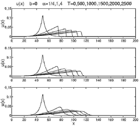
Figure 13: Effect of increasing $\alpha$ for $b=0$. Viscous $b$-family, $b=0$, $\alpha=1/4,1,4$, $\nu=0.005$, initial width $w=5$.

Figure 14 shows three plots of the same type of evolution from a peakon initial condition of width $w=5$, as $\alpha$ is varied for $b=1$. The front of the ramp and cliff structure propagates faster and is sharper for $b=1$ than for $b=0$ when $\alpha=1/4$ and $\alpha=1$. This increase in speed appears to occur because the coefficient increases in the steepening term $(b+1)uu_{x}$ in equation (6). A nascent peakon begins to form close behind the front at the top of the ramp, then eventually gets absorbed into the ramp and cliff. For $\alpha=4$, however, this nascent peakon forms more completely and nearly escapes.

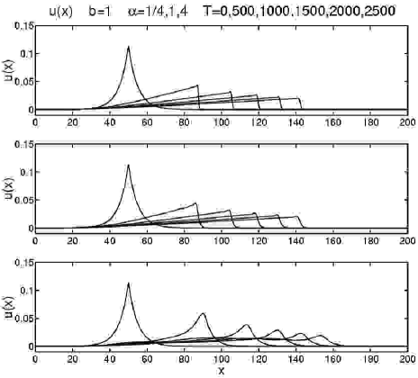
Figure 14: Effect of increasing $\alpha$ for $b=1$. Viscous $b$-family, $b=1$, $\alpha=1/4,1,4$, $\nu=0.005$, initial width $w=5$.

Figure 15 again shows three plots of the evolution from a peakon initial condition of width $w=5$, as $\alpha$ is varied, this time for $b=2$. The ramp and cliff structure is faster for $b=2$ than for $b=1$ when $\alpha=1/4$. When $\alpha=1$ a series of three nascent peakons forms close behind the front, then overtakes the ramp and cliff structure and slightly affects its propagation before eventually being absorbed. For $\alpha=4$, however, the initial peakon simply propagates and decays under viscosity, although it is slightly rounded at the top.

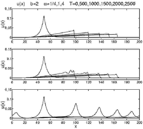
Figure 15: Effect of increasing $\alpha$ for $b=2$. Viscous $b$-family, $b=2$, $\alpha=1/4,1,4$, $\nu=0.005$, initial width $w=5$.

Figure 16 also shows three plots of the evolution from a peakon initial condition of width $w=5$, as $\alpha$ is varied, this time for $b=3$. The ramp and cliff structure moves faster yet, and a single nascent peakon appears just behind the front already for $\alpha=1/4$. When $\alpha=1$, a series of three nascent peakons forms initially close behind the front and they nearly escape before being slowed by viscosity. The leading peakon decays and slows due to viscosity. Then the following ones overtake and collide with the ones ahead as the ramp and cliff structure forms. These collisions occur at higher relative velocity for $b=3$ than for $b=2$ and they significantly affect the propagation and eventual formation of the ramp and cliff. In contrast, for $\alpha=4$, the initial peakon keeps its integrity and simply propagates rightward and decays under viscosity. The propagating peakon for $\alpha=4$ at this viscosity decays more slowly and is much sharper at the top for $b=3$ than for $b=2$.

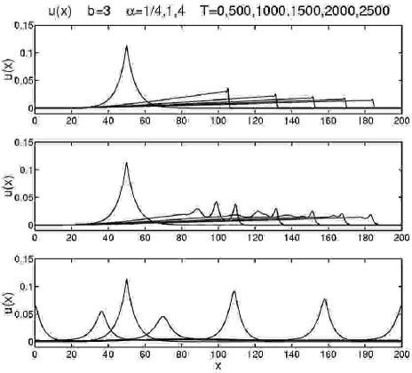
Figure 16: Effect of increasing $\alpha$ for $b=3$. Viscous $b$-family, $b=3$, $\alpha=1/4,1,4$, $\nu=0.005$, initial width $w=5$.

Remark 7.1 (Exchange of stability)

To see the exchange of stability between the ramp/cliff structure and the peakon as $b$ changes, we perform the following numerical experiment. First, we run the viscous b-equation (95) with $b=0$, $\alpha=1$, $\nu=10^{-5}$, and an initial peakon of width $w=5$. As we see in Figures 17 and 18, this evolves into the ramp and cliff formation even for nearly zero viscosity. Once the final ramp/cliff state is formed, we then use it as the new initial condition for equation (95) with either $b=2$ or $b=3$. The new evolution breaks the ramp/cliff structure into peakons and the new final state is a rightward moving train of peakons ordered by height.

For Figures 19 and 20, we ran the same numerical experiment, this time with a value $\alpha=5$ equal to the width of the initial peakon. The initial peakon “borrows from the negative” to form a ramp, which is not quite antisymmetric because the total area of the initial peakon must be preserved. At time $T=150$ we switch to $b=2$ (top plot) or $b=3$ (bottom plot), and again observe a train of stable peakons emerging from the now-unstable ramp.

Finally, for Figures 21 and 22, we again run the numerical experiment with $\alpha=1$ and an initial peakon width $w=5$, but this time changing to $b=-2$ or $b=-3$ after the ramp has formed. The new evolution breaks the ramp/cliff structure into leftons like those in Figures 6 and 7.

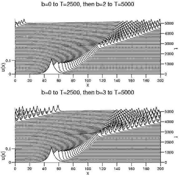
Figure 17: Exchange of stability between ramps and peakons for $b=0,2,3$, when width $>\alpha$. Viscous $b$-family, $b=0\rightarrow 2,3$, $\alpha=1$, $\nu=10^{-5}$, initial width $w=5$.

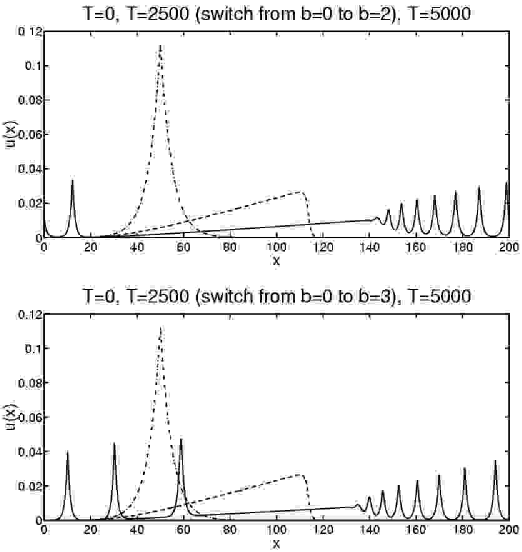
Figure 18: Exchange of stability between ramps and peakons for $b=0,2,3$, when width $>\alpha$: profiles. Viscous $b$-family, $b=0\rightarrow 2,3$, $\alpha=1$, $\nu=10^{-5}$, initial width $w=5$.

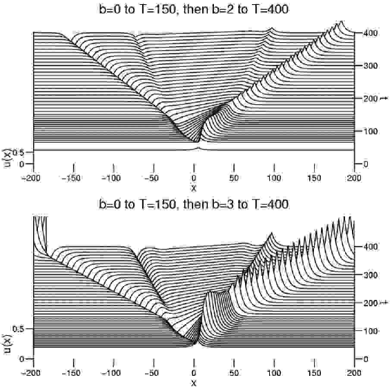
Figure 19: Exchange of stability between ramps and peakons for $b=0,2,3$, when width $=\alpha$. Viscous $b$-family, $b=0\rightarrow 2,3$, $\alpha=5$, $\nu=10^{-5}$, initial width $w=5$.

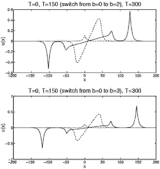
Figure 20: Exchange of stability between ramps and peakons for $b=0,2,3$, when width $=\alpha$: profiles. Viscous $b$-family, $b=0\rightarrow 2,3$, $\alpha=5$, $\nu=10^{-5}$, initial width $w=5$.

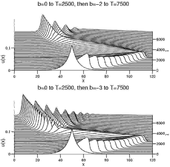
Figure 21: Exchange of stability between ramps and leftons for $b=0,-2,-3$, when width $>\alpha$. Viscous $b$-family, $b=0\rightarrow-2,-3$, $\alpha=1$, $\nu=10^{-5}$, initial width $w=5$.

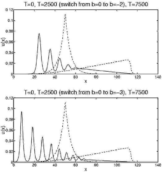
Figure 22: Exchange of stability between ramps and leftons for $b=0,-2,-3$, when width $>\alpha$: profiles. Viscous $b$-family, $b=0\rightarrow-2,-3$, $\alpha=1$, $\nu=10^{-5}$, initial width $w=5$.

Remark 7.2 (Increasing viscosity)

The effect of increasing viscosity on the evolution of the peakon initial condition can be estimated from the $\alpha-$scale Reynolds number defined by,

$$Re_{\alpha}=U\alpha/\nu=(\alpha/\Delta{x})Re_{\Delta{x}}\,.$$

For $(\alpha/\Delta{x})=40$, $U=0.1$ and increasing viscosity $\nu$, the Reynolds numbers $Re_{\Delta{x}}$ and $Re_{\alpha}$ decrease as

$$Re_{\Delta{x}}\simeq 2,0.2,0.02\quad\hbox{and}\quad Re_{\alpha}=\simeq 80,8,0.8\quad\hbox{for}\quad\nu=0.01,0.1,1.0\,.$$

Perhaps not surprisingly, when $Re_{\alpha}=O(1)$ the viscosity will diffuse through the initial peakon before it can fully form. Figures 23 and 24 show that this effect increases as $Re_{\alpha}$ decreases.

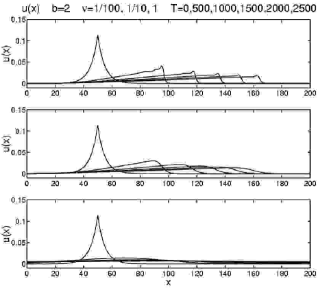
Figure 23: Effect of increasing viscosity for $b=2$. Viscous $b$-family, $b=2$, $\alpha=1$, $\nu=1/100,1/10,1$, initial width $w=5$.

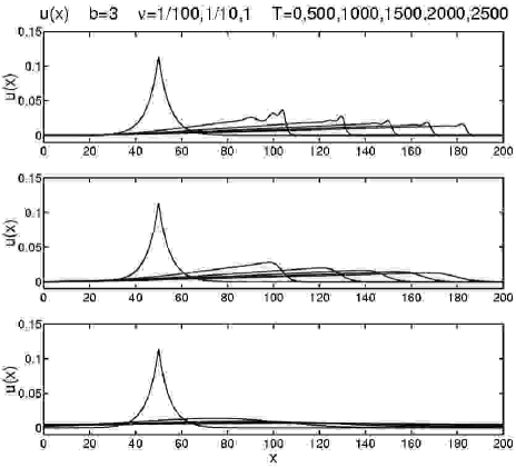
Figure 24: Effect of increasing viscosity for $b=3$. Viscous $b$-family, $b=3$, $\alpha=1$, $\nu=1/100,1/10,1$, initial width $w=5$.

7.2 The fate of peakons under Burgers$-\alpha\beta$ evolution

Figures 25 and 26 show the effects on the peakon initial value problem for the Burgers$-\alpha\beta$ evolution of varying $\alpha$ and $b$ with $(3-b)\beta=1$ at constant viscosity. We shall consider the following cases with $(3-b)\beta=1$:

$b=0$, $\beta=1/3$, $\nu=0.005$, $\alpha=1/4,1,4$, and

$b=1$, $\beta=1/2$, $\nu=0.005$, $\alpha=1/4,1,4$.

Remark 7.3 (Lowering $\beta$ has little effect on the ramp/cliff)

Lowering $\beta$ to follow $(3-b)\beta=1$ instead of keeping $\beta=1$ has little effect on the development of the ramp/cliff solution for $b=0$ and $b=1$. Lowering $\beta$ for these cases only makes the activity slightly less lively at the front for ($b=0$, $\beta=1/3$) and ($b=1$, $\beta=1/2$) than for the corresponding cases of $b=0$ and $b=1$ with $\beta=1$ in Figures 13 and 14. This lessened activity at lower $\beta$ can only be discerned in the solution for the largest value $\alpha=4$. The remaining case (b=2, $\beta=1$) recovers the viscous b-equation (95) for $b=2$ in Figure 15, in which the larger $b$ produces much livelier steepening and, hence, more activity at the front of the rightward moving pulses.

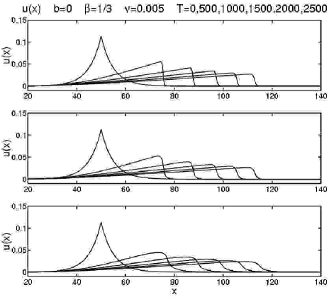
Figure 25: Effect of increasing $\alpha$ when $(3-b)\beta=1$, for $b=0$ and $\beta=1/3$. Burgers-$\alpha\beta$, $b=0$, $\alpha=1/4,1,4$, $\beta=1/3$, $\nu=0.005$, initial width $w=5$.

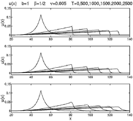
Figure 26: Effect of increasing $\alpha$ when $(3-b)\beta=1$, for $b=1$ and $\beta=1/2$. Burgers-$\alpha\beta$, $b=1$, $\alpha=1/4,1,4$, $\beta=1/2$, $\nu=0.005$, initial width $w=5$.

8 Numerical results for peakon scattering and initial value problems

We shall begin by summarizing the results in the figures given earlier, and then describe the numerical methods used in producing them and discuss some of the ways we verified and validated the results.

8.1 Peakon initial value problems

8.1.1 Inviscid b-family of equations

Ramps and cliffs for $b=0$. Figure 1 shows the formation of a ramp and cliff pattern for $b=0$, $\alpha=1$, and a set of Gaussian initial conditions of increasing width $w=2.5,5,10$.

Peakons for $b=2,3$. Figures 2 and 3 show the formation of peakons for $b=2$ and $b=3$, for $\alpha=1$ and a set of Gaussian initial conditions of increasing width $w=2.5,5,10$.

Ramps and cliffs for $b=-1/2$. Figure 4 shows the formation of a ramp and cliff pattern for $b=-1/2$, $\alpha=1$, and a set of Gaussian initial conditions of increasing width $w=10,15,20$.

Stationary solutions for $b\leq-1$. Figure 5 shows an essentially stationary solution with a slight rightward drift and leaning slightly to the right due to nonlinear curvature terms with higher order derivatives in equation (3.4.2), for $\alpha=1$ and a set of Gaussian initial conditions of increasing width $w=10,15,20$. For the same $\alpha$ and same set of initial conditions, Figures 6 and 7 show the emergence of leftons.

Figure 8 shows the leftons at time $T=2500$ for the $b=-2$ case, versus the analytical $u(x)\simeq{\rm sech}^{2}(x/(2\alpha))$ from equation (53), and for the $b=-3$ case, versus the analytical $u(x)\simeq{\rm sech}(x/\alpha)$.

Peakons of width $\alpha$ for $b=2,3$. Figures 9 and 10 show 2-peakon and 3-peakon interactions for $b=2$ and for $b=3$, beginning with initial peakons of width $w=\alpha=5$.

Peakons of width $>\alpha$ for $b=2,3$. Figure 11 shows the emergence of peakons of width $\alpha=1$ when we begin with peakons of width $w=5$ greater than $\alpha$, for $b=2$ and $b=3$.

Peakon-antipeakon collisions for $b=1,2,3$. Figure 12 shows the dynamics of a peakon-antipeakon collision for $b=1$, $b=2$, and $b=3$, for $\alpha=1$, at four successive times.

8.1.2 Viscous b-family of equations

Effect of $\alpha$ for $b=0,1,2,3$. Figures 13 – 16 show the evolution of an initial peakon of width $w=5$ as a function of increasing $\alpha=1/4,1,4$ at fixed viscosity $\nu=0.005$, for $b=0$, $b=1$, $b=2$, and $b=3$.

Exchange of stability between ramps and peakons. Figures 17 and 18 show the exchange of stability between ramps and peakons suggested in the previous four figures, with $\alpha=1$ and an initial peakon of width $w=5$, but this time with a very small viscosity $\nu=10^{-5}$ so that the peakons, when stable, do not noticeably decay. The exchange of stability occurs when we switch from $b=0$ to $b=2$ or $b=3$. Figures 19 and 20 again show the exchange of stability, this time using $\alpha=5$ so that the initial peakon has width $\alpha$.

Exchange of stability between ramps and leftons. Figures 21 and 22 show the exchange of stability as in Figures 17 and 18, but we switch to $b=-2$ or $b=-3$ instead, and see the emergence of stable leftons from the ramp.

Effect of viscosity for $b=2,3$. Figures 23 and 24 show the effect of increasing viscosity $\nu=0.01,0.1,1$ on the evolution of an initial peakon of width $w=5$, with $\alpha=1$ and $b=2$ or $b=3$.

8.1.3 Burgers-$\alpha\beta$ equation

Effect of $\alpha$ when $(3-b)\beta=1$. Figures 25 and 26 show the effect of increasing $\alpha=1/4,1,4$ on the evolution of an initial peakon of width $w=5$, for fixed $\nu=0.005$ and two sets of values for $b$ and $\beta$ for which $(3-b)\beta=1$: $b=0$, $\beta=1/3$ for the first figure, and $b=1$, $\beta=1/2$ for the second figure.

8.2 Description of our numerical methods

For our numerical runs we advanced equations (84), (99), and (100) with an explicit, variable timestep fourth/fifth order Runge-Kutta-Fehlberg (RKF45) predictor/corrector. We selected the timestep for numerical stability by trial and error, while our code selected the timestep for numerical accuracy (not to exceed the timestep for numerical stability) according to the well-known formula from numerical analysis,

$$h_{i}=\gamma h_{i-1}\left(\frac{\epsilon|h_{i-1}|}{||\bar{u}_{i}-\hat{u}_{i}||}\right)^{1/p}\,.$$ (111)

This is used in the following way. At step $i$ of the calculation, we know the predicted solution $\bar{u}_{i}$, the corrected solution $\hat{u}_{i}$, and the previous timestep $h_{i-1}$. The predictor’s order of accuracy is $p=4$, while the corrector’s order of accuracy is $p+1$. A new timestep $h_{i}$ is chosen from (111) based on the old timestep $h_{i-1}$ and the norm of the difference between the current predicted and corrected solutions. We used a very strict relative error tolerance per timestep, $\epsilon=10^{-8}$, a safety factor $\gamma=0.9$, and an $L_{2}$ norm $||\cdot||_{2}$.

We computed spatial derivatives using 4th order finite differences, generally at resolutions of $2^{13}=8192$ or $2^{14}=16384$ zones. To invert the Helmholtz operator in transforming between $m(x,t)$ and $u(x,t)$, we convolved $m(x,t)$ with the Green’s function in Fourier space. When the numerical approximation of the nonlinear terms had aliasing errors in the high wavenumbers, we applied the following high pass filtered artificial viscosity,

$$\nu(k)=\begin{cases}0&\hbox{if\ \ }0\leq k\leq\frac{N}{3},\cr\frac{3\delta}{N}\left(k-\frac{N}{3}\right)&\hbox{if\ \ }\frac{N}{3}<k<\frac{2N}{3},\cr\delta&\hbox{if\ \ }\frac{2N}{3}\leq k\leq N,\cr\end{cases}$$ (112)

where $\delta=0.01$ for the present simulations. $N$ is one-half the number of zones, because for each zone we have both a Fourier sine coefficient and a Fourier cosine coefficient.

The quality of the numerical convergence may be checked analytically in the case of rear-end two-pulson collisions, for which equation (76) in Corollary 4.4 yields

$$g(q_{min})=g(q)\Big{|}_{p=0}=1-\Big{(}\,\frac{4c_{1}c_{2}}{(c_{1}+c_{2})^{2}}\Big{)}^{{1}/(b-1)}.$$ (113)

For peakons with $b=2$ and $g(x)=e^{-|x|/\alpha}$, this formula gives the minimum separation,

$$q_{min}=-2\alpha\,{\rm ln}\Big{(}\,\frac{c_{1}-c_{2}}{c_{1}+c_{2}}\Big{)}>0\,.$$ (114)

When $c_{1}=1$, $c_{2}=1/2$, and $\alpha=5$, as in figure 9, this formula implies $q_{min}=10\,{\rm ln}\,3=10.9861$. Our numerical results with the resolution of $2^{14}$ zones yield $q_{min}=11.0049$. The very small discrepancy, less than $0.2\%$, occurs largely because our numerical measurement of $q_{min}$ is obtained by examining the peakon positions at each internal timestep in the code, while the code’s time discretization effectively means we’re unlikely to land exactly on the time at which the minimum separation occurs. The code’s true accuracy is thus better than the above measure indicates, because the intermediate steps involved in advancing the solution from one discrete time to the next with an RKF45 method cancel the higher-order discretization errors.

Likewise, for peakons with $b=3$ and $g(x)=e^{-|x|/\alpha}$, formula (113) gives the minimum separation,

$$q_{min}=-\alpha\,{\rm ln}\Big{(}\,1-\frac{\sqrt{c_{1}c_{2}}}{(c_{1}+c_{2})/2}\Big{)}>0\,.$$ (115)

When $c_{1}=1$, $c_{2}=1/2$, and $\alpha=5$, as in figure 10, this formula implies $q_{min}=5\,{\rm ln}\,(3/(3-\sqrt{8}))=14.3068$. This time our numerical results yield $q_{min}=14.2924$, a discrepancy of only $0.1\%$.

Of course, the two-body collision is rather simple compared to the plethora of other multi-wave dynamics that occurs in this problem. For this reason, we also checked the convergence of our numerical algorithms by verifying that the relative phases of the peakons in the various figures remained invariant under grid refinement. Moreover, the integrity of the waveforms in our figures attests to the convergence of the numerical algorithm – after scores of collisions, the waveforms given by the Green’s function for each case are still extremely well preserved. The preservation of these soliton waveforms after so many collisions would not have occurred unless the numerics had converged well.

9 Conclusions

Equation (1) introduced a new family of reversible, parity invariant, evolutionary 1+1 PDEs describing motion by active transport

$$m_{t}\ +\ \underbrace{\ \ um_{x}\ \ }_{\hbox{convection}}\ +\ \underbrace{\ \ b\,u_{x}m\ \ }_{\hbox{stretching}}\ =\ 0\,,\quad\hbox{with}\quad u=g*m\,.$$ (116)

We analyzed the transformation properties and conservation laws of this family of equations, which led us to choose $g$ to be an even function. Then we classified its traveling waves, identified the bifurcations of its traveling wave solutions as a function of the balance parameter $b$ and for some choices of the convolution kernel $g(x)$ we studied its particle-like solutions and their interactions when $b>1$. These were obtained by superposing $N$ traveling wave solutions $u(x,t)=cg(x-ct)$ as

$$u(x,t)=\sum_{i=1}^{N}p_{i}(t)g(x-q_{i}(t))\quad\hbox{and}\quad m(x,t)=\sum_{i=1}^{N}p_{i}(t)\delta(x-q_{i}(t))\,,$$ (117)

for any real constant $b$ and $u=g*m$, in which the function $g$ is even $g(-x)=g(x)$, so that $g\,^{\prime}(0)=0$, and is bounded, so we may set $g(0)=1$.

Following [7], we call these solutions “pulsons.” We have shown that for any $b>1$, once they are initialized on their invariant manifold (which may be finite dimensional), the pulsons undergo particle-like dynamics in terms of the moduli variables $p_{i}(t)$ and $q_{i}(t)$, with $i=1,\dots,N$. The pulson dynamics we studied for $b>1$ in this framework on a finite-dimensional invariant manifold displayed all of the classical soliton interaction behavior for pulsons found in [7] for the case $b=2$. This behavior included pairwise elastic scattering of pulsons, dominance of the initial value problem by confined pulses and asymptotic sorting according to height – all without requiring complete integrability. Thus, the “emergent pattern” for $b>1$ in the nonlinear evolution governed by the active transport equation (1) was the rightward moving pulson train, ordered by height. Thus, the moduli variables $p_{i}(t)$ and $q_{i}(t)$ are collective coordinates on an invariant manifold for the PDE motion governed by equation (1). Once initialized for $b>1$, these collective degrees of freedom persist and emerge as a train of stable pulses, arranged in order of their heights, that then undergo particle-like collisions.

In contrast, the emergent pattern in the Burgers parameter region $0\leq{b}<1$ is the classic ramp/cliff structure as in Figure 13. That the behavior should depend on the value of $b$ is clear from the velocity form of equation (1) written in (6),

$$u_{t}+(b+1)uu_{x}-\nu u_{xx} = \alpha^{2}(u_{xxt}+uu_{xxx}+bu_{x}u_{xx}-\nu u_{xxxx})$$

$$= \alpha^{2}\partial_{x}\Big{(}u_{xt}+uu_{xx}-\nu u_{xxx}+\frac{b-1}{2}u_{x}^{2}\Big{)}$$

$$= \alpha^{2}\partial_{x}^{2}\Big{(}u_{t}+uu_{x}-\nu u_{xx}+\frac{b-3}{2}u_{x}^{2}\Big{)}\,.$$

Thus, nonlinear terms in this equation change sign at four integer values of the parameter $b$. Nonlinear $\alpha^{2}-$terms change sign when $b=0,1,3$. Also, the nonlinear steepening term increases with $b$ as $(b+1)uu_{x}$. So this term changes sign when $b=-1$. In the parameter regime $b>-1$ (resp. $b<-1$) the solutions of equation (1) move rightward (resp. leftward), provided the terms on the right hand side of equation (9) are sufficiently small.

Three regions of $b$.

We found that the solution behavior for equation (1) changes its character near the boundaries of the following three regions in the balance parameter $b$.

(B1) In the stable pulson region $b>1$, the Steepening Lemma for peakons proven for $1<b\leq 3$ in Proposition 5.1 allows inflection points with negative slopes to escape verticality by producing a jump in spatial derivative at the peak of a traveling wave that eliminates the inflection points altogether. Pulson behavior dominates this region, although ramps of positive slope are also seen to coexist with the pulsons. When $b\leq 1$ we found the solution behavior of the active transport equation (1) changed its character and excluded the pulsons entirely.

(B2) In the Burgers region $0\leq{b}\leq 1$, the $L^{1/b}$ norm of the variable $m$ is controlled and the solution behavior is dominated by ramps and cliffs, as for the usual Burgers equation. Similar ramp/cliff solution properties hold for the region $-1\leq{b}\leq 0$, for which the $L^{1/b}$ norm of the variable $1/|m|$ is controlled. At the boundary of the latter region, for $b=-1$, the active transport equation (1) admits stationary plane waves as exact nonlinear solutions.

(B3) In the steady pulse region $b<-1$, pulse trains form that move leftward from a positive velocity initial condition (instead of moving rightward, as for $b>-1$). These pulse trains seem to approach a steady state.

Effects of viscosity.

Almost any numerical investigation will introduce some viscosity or other dissipation. Consequently, we studied the fate of the peakons when viscosity was added to the b-family in equation (95). Viscous solutions of equation (95) for the peakon case $g(x)=e^{-|x|/\alpha}$ with $\alpha=1$ were studied in each of the three solution regions (B1)-(B3). In the Burgers region (B2) near $b=0$ we focused on the shock-capturing properties of the solutions of equation (1) and this family of equations was extended for $\beta\neq 1$ to the Burgers$-\alpha\beta$ equation (100),

$$u_{t}+uu_{x}-\nu u_{xx}=-\,\beta\,\tau_{x}\quad\hbox{with}\quad(1-\alpha^{2}\partial_{x}^{2})\tau=\frac{b}{2}u^{2}+\frac{3-b}{2}\alpha^{2}u_{x}^{2}\,.$$ (119)

According to Proposition 6.1, the Burgers$-\alpha\beta$ equation (119) controls the $\alpha-$weighted $H^{1}$ norm of the velocity for $\alpha^{2}\neq 0$, provided $(3-b)\beta=1$. This analytical property guided our study of this new equation by identifying a class of equations for which a priori estimates guarantee continuity of the solution $u(x,t)$. The shock-capturing properties of the Burgers$-\alpha\beta$ equation (119) and its $\alpha\to\infty$ limit will be reported in a later paper [10].

10 Acknowledgements

We are grateful to A. Degasperis, A. N. W. Hone, J. M. Hyman, S. Kurien, C. D. Levermore, R. Lowrie and E. S. Titi for their thoughtful remarks, careful reading and attentive discussions that provided enormous help and encouragement during the course of writing this paper.

References

- [1] R. Beals, D. H. Sattinger and J. Szmigielski, Multipeakons and the classical moment problem Adv. in Math. 154 (2000) 229-257.
- [2] R. Camassa and D. D. Holm, An integrable shallow water equation with peaked solitons, Phys. Rev. Lett. 71 (1993) 1661-1664, http://xxx.lanl.gov/abs/patt-sol/9305002.
- [3] S. Chen, C. Foias, D. D. Holm, E. J. Olson, E. S. Titi and S. Wynne, The Camassa-Holm equations as a closure model for turbulent channel and pipe flows. Phys. Rev. Lett., 81 (1998) 5338-5341, http://xxx.lanl.gov/abs/chao-dyn/9804026.
- [4] A. Degasperis, D.D. Holm and A.N.W. Hone, A new integrable equation with peakon solutions. Submitted to NEEDS Proceedings, 2001. To appear (2002).
- [5] A. Degasperis and M. Procesi, Asymptotic integrability, in Symmetry and Perturbation Theory, edited by A. Degasperis and G. Gaeta, World Scientific (1999) pp.23-37.
- [6] H. Dullin, G. Gottwald and D. D. Holm, An integrable shallow water equation with linear and nonlinear dispersion. Phys. Rev. Lett. 87 (2001) 194501-04.
- [7] O. Fringer and D. D. Holm, Integrable vs. nonintegrable geodesic soliton behavior. Physica D 150 (2001) 237-263, http://xxx.lanl.gov/abs/solv-int/9903007.
- [8] D. D. Holm, J. E. Marsden and T. S. Ratiu, The Euler–Poincaré equations and semidirect products with applications to continuum theories. Adv. in Math. 137 (1998) 1-81.
- [9] D. D. Holm, J. E. Marsden and T. S. Ratiu, Euler–Poincaré models of ideal fluids with nonlinear dispersion. Phys. Rev. Lett. 80 (1998) 4173-4177.
- [10] D. D. Holm, R. B. Lowrie and M. F. Staley, Shock-capturing properties of the Burgers equation. In preparation.
- [11] D. D. Holm and E. S. Titi, PDE results for peakon dynamics. In preparation.
- [12] J. K. Hunter and R. H. Saxton, Dynamics of director fields. SIAM J. Appl. Math. 51 (1991), 1498-1521.