A Theory for Quantum Accelerator Modes in Atom Optics

Abstract

Unexpected accelerator modes were recently observed experimentally for cold cesium atoms when driven in the presence of gravity. A detailed theoretical explanation of this quantum effect is presented here. The theory makes use of invariance properties of the system, that are similar to the ones of solids, leading to a separation into independent kicked rotor problems. The analytical solution makes use of a limit that is very similar to the semiclassical limit, but with a small parameter that is not Planck’s constant, but rather the detuning from the frequency that is resonant in absence of gravity.

1 Introduction

The kicked rotor is a standard system used in the investigation of classical Hamiltonian chaos and its manifestations in quantum mechanical systems [1, 2, 3]. The motion is classically described by the Standard Map. The size of the chaotic component in the phase space of this map increases with the driving strength, and when the latter is sufficiently strong unbounded diffusion in action space takes place. Important deviations are however found for some values of the driving strength [2, 3, 4], due to the onset of so-called accelerator modes, that produce linear, rather than diffusive, growth of momentum along orbits in a set of positive measure. Quantization imposes remarkable modifications. For typical parameter values, the classical diffusion is quantally suppressed by a mechanism that is similar to Anderson localization in disordered solids [1, 5]. The accelerator modes decay in time due to quantum tunneling [6]. Quantum resonances are found when the natural frequency of the rotor is commensurate with the frequency of the driving [7]. The quasienergy states are then extended in angular momentum, leading to ballistic (i.e., linear) growth of the latter in time.

The quantal suppression of classical diffusive transport first observed in the quantum kicked rotor is actually a more general phenomenon, now known as dynamical localization. Theoretical predictions [8] prompted the first experimental observations of this phenomenon for microwave driven Hydrogen and Hydrogen like atoms[9].

The most direct experimental realization of the quantum kicked rotor is achieved in the field of atom optics, by a technique pioneered by Raizen and coworkers [10]. Laser-cooled Atoms (first Sodium and later Cesium) are driven by application of a standing electromagnetic wave. The frequency of the wave is slightly detuned from resonance, so a dipole moment is induced in the atom. This moment couples with the driving field, giving rise to a net force on the center of mass of the atoms, proportional to the square of the electric field [11, 12]. As the wave is periodic in space, the atom is thus subjected to a periodic potential. The wave is turned on and off periodically in time, and the time it is on is much shorter then the time it is off. A realization of a periodically kicked particle is then obtained. In real experiments the duration of the kicks is always finite, setting a bound on the the momentum range wherein the $\delta$-kicked model is applicable. At very large momentum the driving becomes adiabatic, leading to trivial classical and quantum localization in momentum [13, 10].

The basic difference between the kicked particle and the kicked rotor is that the momentum of the particle is not discrete as is the angular momentum of the rotor. As we shall review in Sect.(2.2) , this difference is circumvented by Bloch theory. The spatial periodicity of the driving only allows for transitions between momenta that differ by integer multiples of $\hbar G$, with $2\pi G^{-1}$ the spatial period of the driving potential. This implies conservation of quasi-momentum. The particle wavepacket is a continuous superposition of states with given quasi-momenta. The dynamics at any one fixed quasi-momentum is that of a rotor, which however differs from the standard kicked rotor because of a constant shift in the angular momentum eigenvalues, proportional to the given quasi-momentum. This modification of the kicked rotor dynamics is formally the same as that produced by a Aharonov-Bohm flux threading the rotor. It does not crucially affect dynamical localization [14], so the latter carries over to the particle dynamics. In experiments [10] it is found that for typical values of the parameters, an initial narrow gaussian distribution around zero momentum spreads into an exponential distribution, characteristic of dynamical or Anderson localization.

The difference between the rotor’s and the particle’s dynamics due to the presence of a continuum of quasi-momenta is indeed crucial in what concerns quantum resonances at “commensurate” values of the kicking period, because these only occur at special values of quasi-momentum. Therefore, nearly all quasi-momenta involved in a particle’s wave packet would not be in resonance [15]. In this paper we present an exact calculation, showing that the quadratic spread in momentum grows in this case linearly in time, in contrast to the situation found for the kicked rotor, where this spread is quadratic in time. A more detailed analysis of the kicked particle dynamics at resonance will be presented elsewhere [16].

In the above discussed experiments, gravity had but negligible effects, as driving of the atoms took place in the horizontal direction. In recent experiments [17, 18, 19], that provide the subject of the theoretical analysis of the present paper, atoms were driven in the vertical direction, and gravity was found to produce remarkable effects. In the vicinity of the resonant frequencies of the kicked rotor, a new type of ballistic spread in momentum was experimentally observed [17, 18, 19]. A fraction of the atoms are steadily accelerated, at a rate which is faster or slower than the gravitational acceleration depending on what side of the resonance the driving frequency is. Such atoms are exempt from the diffusive spread that takes place for the other atoms, and their acceleration depends on the difference between the driving and the resonant frequencies. In ref. [18] a physical explanation was given, and it was stressed that the phenomenon is resemblant of the accelerator modes in the Standard Map. The accelerating parts of the distributions were hence termed “quantum accelerator modes”, at once emphasizing that resemblance, and their purely quantal nature; in fact, they have no classical counterpart in the classical dynamics of the kicked particles in gravity.

In this paper we present a theory that explains the experimental results in terms of the exact quantum equations of motion, and allows for further predictions. The main result is that the quantum accelerator modes in presence of gravity do indeed correspond to accelerator modes of a classical map. This map is not, however, the one given by the proper classical limit $(\hbar\to 0)$. It emerges of a quasi-classical asymptotics, where the small parameter is not $\hbar$ but rather the detuning of the kicking frequency from the resonance of the kicked rotor. Though a formally simple variant of the Standard Map, it is endowed with a rich supply of accelerator modes and complex bifurcation patterns.

Our analysis starts from the time-dependent Schrodinger equation for the kicked particle in the laboratory frame. A simple gauge transform reduces the corresponding Floquet operator to that of a particle kicked by a potential, that is quasi-periodic (and not just periodic) in space (Sect.(2.1)). The corresponding incommensuration parameter adds to the kicking period, in building a formidable mathematical problem. In particular, quasi-momentum is not conserved, preventing implementation of the Bloch theory. Moving to a free-falling frame removes this difficulty and restores decomposition into independent rotor problems, at the price of time-dependent Floquet operators (Sect.(2.3)). On such operators we work out the mentioned quasi-classical approximation at small detuning from resonance.

Variants of the kicked-rotor, in which some parameter was allowed to change with time, have been considered earlier [20], the issue being what degree of uncorrelatedness in the time-dependence is sufficient to destroy localization. For the quasi-periodic dependence of the present model, this issue is as yet unsolved, and depends on incommensuration properties. In a mathematical aside of this work, we prove that in the presence of gravity and at resonant values of the kicking period the particle energy (in the falling frame) grows linearly in time, in sufficiently incommensurate cases at least.

2 Discrete-Time Quantum Dynamics

The dynamics of the atoms that are falling as a result of gravity and are kicked by the external field is modeled by the time-dependent Hamiltonian:

$${\hat{H}}(\mathtt{t})=\frac{{\hat{P}}^{2}}{2M}-Mg{\hat{X}}+\kappa\cos(G{\hat{X}})\sum\limits_{t=-\infty}^{+\infty}\delta(\mathtt{t}-tT),$$ (1)

where $\mathtt{t}$ is the continuous time variable, the integer variable $t$ counts the kicks, ${\hat{P}},{\hat{X}}$ are the momentum and the position operator respectively, $M$ is the mass of the atom, $2\pi G^{-1}$ is the spatial period of the kicks, $\kappa$ is the kick strength, and $T$ is the kicking period in time. The positive $x-$direction is that of the gravitational acceleration. Without changing notations, we rescale momentum ${\hat{P}}$ in units of $\hbar G$, position ${\hat{X}}$ in units of $G^{-1}$, and mass in units of $M$. Then the energy $E$ comes in units of $\hbar^{2}G^{2}/M$, and time $\mathtt{t}$ in units of $M/(\hbar G^{2})$. The reduced Planck constant is equal to $1$, and the Hamiltonian takes the following form:

$${\hat{H}}(\mathtt{t})\;=\;\frac{{\hat{P}}^{2}}{2}-\frac{\eta}{\tau}{\hat{X}}+k\cos({\hat{X}})\sum\limits_{t=-\infty}^{+\infty}\delta(\mathtt{t}-t\tau)\;,$$ (2)

where:

$$k\;=\frac{\kappa}{\hbar}\;\;\,\;\;\tau\;=\;\frac{\hbar TG^{2}}{M}\;\;,\;\;\eta\;=\;\frac{MgT}{\hbar G}\;,$$ (3)

In the above defined units, $\eta/\tau$ is the gravitational acceleration. The dynamics is fully characterized by the dimensionless parameters $k,\tau,\eta$.

In the following Dirac notations will be used: e.g., $\psi(x)=\langle x|\psi\rangle$ and $\psi(p)=\langle p|\psi\rangle$ will denote the wave function in the position and in the momentum representation respectively.

2.1 Floquet operators.

The quantum evolution over a sequence of discrete times spaced by one period of the external periodic driving is obtained by repeated application of the Floquet operator. This is the single unitary operator which gives the evolution from any instant to the next one in the given sequence of times. Our discrete times will be the kicking times themselves . Throughout the following, time is a discrete variable, given by the kick counter $t$. As the state discontinuously changes at the kicking times, we further specify the state at time $t$ to be the one immediately after the $t-$th kick. The Floquet operator ${\hat{U}}$ is then found by integrating the Schrödinger equation (with the Hamiltonian (2)) from t$=0_{+}$ to t$=\tau_{+}$:

$${\hat{U}}\;=\;{\hat{K}}{\hat{F}}\;=\;e^{-ik\cos({\hat{X}})}{\hat{F}}\;,$$ (4)

where ${\hat{K}}$ describes the kick, and ${\hat{F}}$ describes free fall inbetween kicks. With the present units, the energy eigenfunctions $u_{E}(p)=\langle p|E\rangle$ of the particle in the gravity field read [21] :

$$u_{E}(p)\;=\;\left(\frac{\tau}{2\pi\eta}\right)^{1/2}\;e^{i\frac{\tau}{\eta}(Ep-\frac{p^{3}}{6})}\;.$$

Therefore, apart from a constant phase factor,

$$\langle p^{\prime}|{\hat{F}}|p^{\prime\prime}\rangle\; = \;\int dE\;e^{-iE\tau}u_{E}(p^{\prime})u^{*}_{E}(p^{\prime\prime})$$

$$= \;\delta(p^{\prime}-p^{\prime\prime}-\eta)\;e^{-i\frac{\tau}{2}(p^{\prime}-\frac{\eta}{2})^{2}}$$

Moreover,

$$\langle p|e^{-ik\cos({\hat{X}})}|p^{\prime}\rangle\;=\;\sum\limits_{n=-\infty}^{\infty}K_{n}\;\delta(p-p^{\prime}-n)\;$$

where $K_{n}=(-i)^{n}J_{n}(k)$ and $J_{n}(k)$ are the Bessel functions of the 1-st kind. Replacing in (4) we get the explicit form of the propagator in the laboratory frame:

$$({\hat{U}}\psi)(p)\;=\;\sum\limits_{n=-\infty}^{\infty}K_{n}\;e^{-i\frac{\tau}{2}(p-n-\frac{\eta}{2})^{2}}\ \psi(p-n-\eta)\;.$$ (5)

Note that $K_{n}=K_{-n}$. A more transparent formulation is gained by introducing the operators:

$${\hat{R}}=e^{-i\tau{\hat{P}}^{2}/2}\;\;,\;\;{\hat{S}}=e^{i\eta{\hat{X}}/2}$$

One may then write:

$${\hat{U}}={\hat{S}}{\hat{K}}{\hat{R}}{\hat{S}}={\hat{S}}^{\dagger}{\hat{U}}^{\prime}{\hat{S}}\;\;\;,\;\;\;{\hat{U}}^{\prime}={\hat{S}}^{2}{\hat{K}}{\hat{R}}$$ (6)

Thus ${\hat{U}}$ only differs by a unitary transformation (in fact a gauge transformation) from ${\hat{U}}^{\prime}$, which has the simple form:

$${\hat{U}}^{\prime}\;=\;=e^{i(\eta{\hat{X}}-k\cos({\hat{X}}))}\;e^{-i\tau{\hat{P}}^{2}/2}$$ (7)

Thus formulated, the problem is that of a particle freely moving on a line, except for time-periodic kicks. The spatial dependence of the kicks is periodic when $\eta$ is rational, quasi-periodic otherwise.

2.2 Quasi-momentum and Kicked Rotors.

If $\eta=0$, then (7) is formally similar to the Kicked Rotor model [1], from which it however differs in one crucial respect: whereas the latter has the kicked particle moving on a circle, (7) has the particle moving on a line instead. A link between the two models is established by the spatial periodicity of the kicking potential. We review this well-known construction, because it plays a fundamental role in this paper.

At $\eta=0$ the evolution operator ${\hat{U}}$ commutes with spatial translations by multiples of $2\pi$. As is well known from Bloch theory, this enforces conservation of quasi-momentum. In our units, this is given by the fractional part of momentum, and will be denoted by $\beta$. We then introduce a family of fictitious rotors (particles moving on a circle) parametrized by $\beta\in[0,1)$, with angle coordinate $\theta$ (henceforth named $\beta-$rotors), and denote $|\Psi_{\beta}\rangle$ their states. For integer $n$ we denote $|n\rangle$ the angular momentum eigenstates of these rotors so that in the $\theta-$ representation $\langle\theta|n\rangle=(2\pi)^{-1/2}\exp(in\theta)$. To states $|\psi\rangle$ of the particle we associate states $|\Psi_{\beta}\rangle$ of the $\beta-$rotors as follows:

$$\langle\theta|\Psi_{\beta}\rangle\;=\;\frac{1}{\sqrt{2\pi}}\sum\limits_{n}\langle n+\beta|\psi\rangle e^{in\theta}\;.$$ (8)

In the angular momentum representation,

$$\langle n|\Psi_{\beta}\rangle\;=\;\langle n+\beta|\psi\rangle$$ (9)

Note that $|\Psi_{\beta}\rangle$ is not necessarily normalized to $1$, even if $|\psi\rangle$ is. Conversely, the state of the particle is retrieved from the $\beta-$rotor states via

$$\langle p|\psi\rangle\;=\;\frac{1}{\sqrt{2\pi}}\int_{0}^{2\pi}d\theta\;\langle\theta|\Psi_{\beta}\rangle\;e^{-in\theta}\;\;,\;\;n=[p]\;\;,\beta=\{p\}\;.$$ (10)

where $[p],\{p\}$ denote the integer and the fractional part of the momentum $p$ respectively. Using (10) and Poisson’s summation formula, one obtains the wave function in the $x-$representation:

$$\langle x|\psi\rangle=\frac{1}{\sqrt{2\pi}}\int dp\;e^{ipx}\langle p|\psi\rangle=\int_{0}^{1}d\beta\;e^{i\beta x}\langle x\;\mbox{\rm mod}(2\pi))|\Psi_{\beta}\rangle\;.$$ (11)

Fixing a sharp value of $\beta$ yields a spatially extended state (a Bloch wave ) for the particle, even with a normalizable rotor wave function.

It follows from (5) and (9) (with $\eta=0$) that as $|\psi\rangle$ evolves into ${\hat{U}}^{t}|\psi\rangle\;$, $|\Psi_{\beta}\rangle$ in turn evolves into ${\hat{\mathcal{U}}}_{\beta}^{t}|\Psi_{\beta}\rangle$, where:

$${\hat{\mathcal{U}}}_{\beta}=({\hat{\mathcal{K}}}{\hat{\mathcal{R}}}_{\beta})\;\;,\;\;\langle n|{\hat{\mathcal{K}}}|m\rangle=K_{n-m}\;\;,\;\;\langle n|{\hat{\mathcal{R}}}_{\beta}|m\rangle=\delta_{nm}\;e^{-i\frac{\tau}{2}(\beta+m)^{2}}\;.$$ (12)

Eqn. (12) may also be written as follows:

$${\hat{\mathcal{U}}}_{\beta}\;=\;e^{-ik\cos({\hat{\theta}})}\;e^{-i\frac{\tau}{2}({\hat{\mathcal{N}}}+\beta)^{2}}.$$ (13)

where ${\hat{\mathcal{N}}}=\sum_{n}n|n\rangle\langle n|$ is the angular momentum operator: ${\hat{\mathcal{N}}}=-i\frac{d}{d\theta}$ in the $\theta-$representation, At $\beta=0$, eqn. (13) is the standard Floquet operator of the Kicked Rotor. At $\beta\neq 0$ one obtains a variant of the Kicked Rotor, which has also been studied, $\beta$ being typically given the physical meaning of an external magnetic flux[14].

We have thus shown that in the presence of conserved quasi-momentum the particle dynamics can be determined as follows: given an initial particle (pure) state $|\psi(0)\rangle$ one first computes the corresponding rotor states $|\Psi_{\beta}(0)\rangle$ as above described. These separately evolve into $|\Psi_{\beta}(t)\rangle$ at time $t$. The particle state $|\psi(t)\rangle$ is finally reconstructed using (10). The process of decomposing the particle dynamics in a bundle of rotors will henceforth be named “the Bloch-Wannier fibration”. It is the quantal counterpart of the classical process of “folding back” the particle trajectory onto a circle, by taking the $x-$coordinate mod$(2\pi)$.

The kinetic energy of the particle at time $t$ is:

$${\mathcal{E}}(t)\; = \;\frac{1}{2}\int dp\;p^{2}|\psi(p,t)|^{2}\;=\;\frac{1}{2}\sum\limits_{n=-\infty}^{\infty}\;\int_{0}^{1}d\beta\;(n+\beta)^{2}|\psi(n+\beta,t)|^{2}$$ (14)

$$= \frac{1}{2}\int_{0}^{1}d\beta\int_{0}^{2\pi}d\theta\left\{\left|\frac{d}{d\theta}\langle\theta|\Psi_{\beta}(t)\rangle\right|^{2}+\beta^{2}|\langle\theta|\Psi_{\beta}(t)\rangle|^{2}+\right.$$

$$- 2i\left.\beta\langle\Psi_{\beta}(t)|\theta\rangle\frac{d}{d\theta}\langle\theta|\Psi_{\beta}(t)\rangle\right\}$$

In the case of unbounded propagation in momentum space, it is the 1st term within the curly brackets which yields the dominant contribution at large $t$ (the 2-nd is bounded by $1$, the 3-d is order of square root of the 1-st.). Note that the 1-st term is the average over $\beta$ of the $\beta-$ rotors kinetic energy.

2.3 Motion in the falling frame.

In the case of nonzero gravity, quasi momentum is not conserved any more because the kicking potential in (7) is not periodic (unless $\eta$ is rational). However, a quasi-momentum -conserving evolution is restored by the substitution :

$$\psi_{f}(p,t)\;=\;\langle p+t\eta|{\hat{U}}^{t}|\psi),$$

Since $\eta$ is the momentum gained over one period due to gravity, this amounts to measuring momentum in the free-falling frame (recall that the positive $x-$direction is that of gravitational acceleration).

From (5) it follows that

$$\psi_{f}(p,t+1)\;=\sum\limits_{n}K_{n}\;e^{-i\frac{\tau}{2}(p-n+t\eta+\frac{\eta}{2})^{2}}\psi_{f}(p-n,t)\;.$$ (15)

that may be rewritten as :

$$|\psi_{f}(t+1)\rangle={\hat{U}}_{f}(t)|\psi_{f}(t)\rangle\;\;,\;\;{\hat{U}}_{f}(t)=e^{-ik\cos({\hat{X}})}e^{-i\frac{\tau}{2}({\hat{P}}+t\eta+\frac{\eta}{2})^{2}}\;.$$ (16)

The operator ${\hat{U}}_{f}(t)$ describes up to a constant phase the evolution from (continuous) time $\mathtt{t}=(t\tau)_{+}$ to time $(\mathtt{t}+\tau)_{+}$ under the time-dependent Hamiltonian

$${\hat{H}}_{f}(\mathtt{t})\;=\;\frac{1}{2}(\hat{P}+\frac{\eta}{\tau}\mathtt{t})^{2}+k\cos(\hat{X})\sum\limits_{t=-\infty}^{+\infty}\delta(\mathtt{t}-t\tau)\;,$$ (17)

that describes the motion in the falling frame. This Hamiltonian is related to that in eqn.(2) by the gauge transformation $e^{i\eta{\hat{X}}\mathtt{t}/\tau}$. The classical dynamics corresponding to (16) is given by the area-preserving, time-dependent map in the $(x,p)$ plane:

$$p_{t+1}=p_{t}+k\sin(x_{t+1})\;\;,\;\;x_{t+1}=x_{t}+\tau(p_{t}+t\eta+\frac{\eta}{2})\;.$$ (18)

Since $\hbar=1$ in our units, the classical limit is approached as

$$k\rightarrow\infty\;,\;\tau\rightarrow 0\;,\;\eta\rightarrow\infty\;,\;k\tau\rightarrow\mbox{\rm const.}\neq 0\;,\;\eta\tau\rightarrow\mbox{\rm const.}\neq 0\;.$$ (19)

The evolution (15) only mixes momenta which differ by integers: hence, quasi-momentum is conserved, so the Bloch-Wannier fibration can be fully implemented, as described in the previous Section. Eqn.(12) now becomes:

$$|\Psi_{\beta}(t)\rangle\;=\;\prod\limits_{r=0}^{t-1}\;{\hat{\mathcal{U}}}_{\beta}(r)|\Psi_{\beta}\rangle\;,\;\;\;{\hat{\mathcal{U}}}_{\beta}(r)={\hat{\mathcal{K}}}{\hat{\mathcal{R}}}_{\beta}(r)$$ (20)

(all operator products ordered from right to left), where

$$\langle n|{\hat{\mathcal{K}}}|m\rangle=K_{n-m}\;\;,\;\;\langle n|{\hat{\mathcal{R}}}_{\beta}(r)|m\rangle=\delta_{nm}\;e^{-i\frac{\tau}{2}(\beta+m+r\eta+\eta/2)^{2}}\;.$$ (21)

Consequently, in the falling frame,

$${\hat{\mathcal{U}}}_{\beta}(t)\;=\;e^{-ik\cos({\hat{\theta}})}\;e^{-i\frac{\tau}{2}({\hat{\mathcal{N}}}+\beta+\eta t+\eta/2)^{2}}.$$ (22)

3 Features of Quantum Dynamics in the falling frame.

The theoretical importance of the Kicked Rotor model lies with its asymptotic properties in time. Best known among these are dynamical localization, and quantum resonances. Though not crucial to current experiments, the long-time asymptotics is an important theoretical question for the present models, too. Apart from resonances, we do not attempt at a thorough theoretical analysis of this issue, which is likely to critically depend on the arythmetic type of $\tau,\eta,\beta$. Though some results in this respect will be presented later, we mostly focus on intermediate-time features of the quantum dynamics, directly connected to experimental findings.

In this section the falling frame is constantly used, without any further reference to the laboratory frame. The suffix _f will be omitted in order to simplify notations.

3.1 Resonances

3.1.1 Zero Gravity

If the kicking period $\tau$ is commensurate to $4\pi$, that is $\tau=4\pi p/q$ with $p,q$ relatively prime integers, and in addition $\beta=m/(2p)$ with $m<2p$ an integer, then the $\beta-$Kicked Rotor exhibits the phenomenon of Quantum Resonance [7]. In that case, indeed, the rotor dynamics commutes with translations in momentum by multiples of $q$. This typically results in band (absolutely continuous) quasi-energy spectrum and ballistic spread of the rotor wave packet in the momentum representation. For special values of $q$ the bands may however be flat. This is the case when $q=2$; the ballistic spread is then only observed at $\beta=1/2$, while at $\beta=0$ the dynamics is sharply localized in momentum (“anti-resonance”), as can be seen from (13), making use of the fact that $e^{-i\pi ln^{2}}=e^{-i\pi ln}$ holds for integer $l$ and $n$. The width of the quasi-energy bands rapidly decreases as the order $q$ of the resonance increases[7]. Ballistic motion is then observed only after quite long times. This places high-order resonances beyond experimental observation. Our discussion is mostly focused on the main resonances ($q=1,2$).

Since the quadratic growth of energy at resonant values of $\tau$ requires a sharp value of quasi-momentum (hence an extended particle state in position), it cannot be observed in the particle wave packet long-time dynamics, not even at resonant values of $\tau$. Nevertheless, with a generic choice of the initial wavepacket, a resonant effect is still manifest, in the form of linear asymptotic growth of the particle energy. This is qualitatively understood as follows. At time $t$, rotors whose quasi-momenta lie within $\sim 1/t$ of the resonant value(s) are still mimicking the resonant growth of energy $\propto t^{2}$. Assuming a smooth initial distribution of quasi-momenta, such rotors enter the average over $\beta$ (14) with a weight $\propto 1/t$. This directly leads to the linear growth of ${\mathcal{E}}(t)$. The latter can also be rigorously proven, and the proportionality factor computed. This is done in the Appendix, under the hypothesis that the initial wave function of the particle is such that $\langle\psi|{\hat{X}}^{2\alpha}|\psi\rangle<\infty$ for some $\alpha>1$.

3.1.2 Nonzero gravity

The $\beta-$rotor dynamics at resonant values of $\tau$ in the presence of gravity is a nontrivial mathematical problem, which may give rise to different types of quantum transport depending on the arythmetic type of $\eta$.

In the Appendix we prove that for $\tau=2l\pi$ ,($l$ integer), and for all irrational $\eta$ in a set of full Lebesgue measure, the energy ${\mathcal{E}}(t)$ (in the falling frame) grows like $k^{2}t/4$, under the hypothesis that the initial wave function satisfies $\langle\psi|{\hat{X}}^{2\alpha}|\psi\rangle<\infty$ for some $\alpha>1$.

3.2 Accelerator Modes

3.2.1 Quantum Rotor Dynamics near Resonance.

We shall now analyze the quantum dynamics at values of $\tau$ close to the resonant values $2\pi l$ ($l>0$ integer) and for large kicking strength $k$. We hence assume $\tau=2\pi l+\epsilon$ with $l$ integer and $|\epsilon|<<1$, and rescale $k={\tilde{k}}/|\epsilon|$. Replacing in (21) and noting $e^{-i\pi ln^{2}}=e^{-i\pi ln}$ we get:

$$\langle m|{\hat{\mathcal{R}}}_{\beta}(t)|n\rangle\;=\;\delta_{mn}\;e^{-i\frac{\tau}{2}(\beta+t\eta+\eta/2)^{2}}\;e^{-i(\epsilon\frac{n^{2}}{2}+n(\pi l+\tau\beta+\tau t\eta+\tau\frac{\eta}{2}))}$$

whence it follows that (apart from an irrelevant phase factor)

$${\hat{\mathcal{U}}}_{\beta}(t)\;=\;e^{-\frac{i}{|\epsilon|}{\tilde{k}}\cos{\hat{\theta}}}\;e^{-\frac{i}{|\epsilon|}{\hat{\mathcal{H}}}_{\beta}({\hat{I}},t)}$$ (23)

where

$${\hat{I}}=|\epsilon|{\hat{\mathcal{N}}}=-i|\epsilon|\frac{d}{d\theta}\;\;\;,\;\;{\hat{\mathcal{H}}}_{\beta}({\hat{I}},t)=\frac{1}{2}\;\mbox{\rm sign}(\epsilon){\hat{I}}^{2}+{\hat{I}}(\pi l+\tau(\beta+t\eta+\frac{\eta}{2}))\;,$$ (24)

If $|\epsilon|$ is assigned the role of Planck’s constant, then (23),(24) is the formal quantization of either of the following classical (time-dependent) maps :

$$I_{t+1}=I_{t}+{\tilde{k}}\sin(\theta_{t+1})\;\;,\;\;\theta_{t+1}=\theta_{t}\pm I_{t}+\pi l+\tau(\beta+t\eta+\eta/2)\;\mbox{\rm mod}(2\pi)\,$$ (25)

where $\pm$ has to be chosen according to the sign of $\epsilon$. The small $|\epsilon|$ asymptotics of the quantum $\beta-$ rotor is thus equivalent to a quasi-classical approximation based on the “classical” dynamics (25). We emphasize that “classical” here is not related to the $\hbar\to 0$ limit but to the limit $\epsilon\to 0$ instead. The two limits are actually incompatible with each other except possibly when $l=0$ (see (19)). For the sake of clarity the term “$\epsilon-$classical” will be used in the following.

3.2.2 $\epsilon-$Classical rotor dynamics.

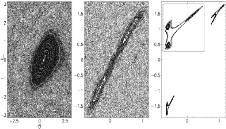
Figure 1: Phase portraits for the map (26) on the 2-torus, with $\tau=5.86,\eta/\tau=0.01579,\epsilon=-0.423$. Here the torus is mapped onto $[-\pi,\pi)\times[-\pi,\pi)$. One stable fixed point with ${\mathfrak{j}}=0$ exists for $0.542<{\tilde{k}}<4.037$. Left: ${\tilde{k}}=1.329$, the stable fixed point is at $J^{*}=0$, $\theta^{*}=0.42$. Center: ${\tilde{k}}=4.232$, a stable period-2, ${\mathfrak{j}}=0$ orbit is visible. Right: ${\tilde{k}}=4.494$, the period-$2$ orbit has left room to a stable period-$6$ orbit. The lower left part is magnified in the inset.

Changing variable to $J_{t}=I_{t}\pm\pi l\pm\tau(\beta+\eta t+\eta/2)$ removes the explicit time dependence of the maps (25), yielding:

$$J_{t+1}=J_{t}+{\tilde{k}}\sin(\theta_{t+1})\pm\tau\eta\;,\;\;\;\theta_{t+1}=\theta_{t}\pm J_{t}\;.$$ (26)

These area-preserving maps are $2\pi$- periodic in $J$ and $\theta$, so they define smooth, area-preserving maps of the 2-torus parametrized by ${\cal J}=J$ mod$(2\pi)$, $\vartheta=\theta$ mod$(2\pi)$. Such “toral maps” are conjugated to each other under ${\cal J}\to 2\pi-{\cal J}$ mod$(2\pi)$, $\vartheta\to\vartheta+\pi$ mod$(2\pi)$. They differ from the Standard Map by the constant drift $\eta\tau$.

Let ${\cal J}_{0},\vartheta_{0}$ be a period-${\mathfrak{p}}$ fixed point of either toral map. Iterating (26) with $J_{0}={\cal J}_{0}\;,\;\theta_{0}=\vartheta_{0}$, at $t={\mathfrak{p}}$ one obtains:

$$J_{{\mathfrak{p}}}=J_{0}+2\pi{\mathfrak{j}}\;\;,\;\;\theta_{{\mathfrak{p}}}=\theta_{0}+2\pi n$$ (27)

for some integers ${\mathfrak{j}}\;,\;n$. The points $({\cal J}_{t},\vartheta_{t})$ with $0\leq t\leq{\mathfrak{p}}-1$ are period-${\mathfrak{p}}$ fixed points themselves, and define a period-${\mathfrak{p}}$ periodic orbit of the toral map, which is primitive if all such points are distinct.

Period-$1$ fixed points are given on the 2-torus by ${\cal J}_{0}=0$, $\vartheta_{0}=\theta_{{\mathfrak{j}}}$, where

$$\sin(\theta_{{\mathfrak{j}}})\;=\;\frac{2\pi{\mathfrak{j}}\mp\tau\eta}{{\tilde{k}}}$$ (28)

and ${\mathfrak{j}}$ is any integer such that:

$$-{\tilde{k}}\pm\tau\eta\leq 2\pi{\mathfrak{j}}\leq{\tilde{k}}\pm\tau\eta\;.$$ (29)

No such point exists if ${\tilde{k}}<\tau\eta<\pi$; two (at least) exist (that is, (28) is solvable for at least one value of the integer ${\mathfrak{j}}$) whenever ${\tilde{k}}\geq\pi$. Two period-$1$ fixed points with ${\mathfrak{j}}=0$ exist whenever ${\tilde{k}}\geq\tau\eta$. In order for the period-$1$ fixed points (28) to be stable it is required that:

$$-4\;<\;\pm{\tilde{k}}\cos(\vartheta_{0})\;<\;0$$ (30)

From (29), (30) it follows that for any integer ${\mathfrak{j}}$ each map (26) has exactly one stable period-$1$ fixed point on the 2-torus, given by (28) if, and only if,

$${{\tilde{k}}}^{({\mathfrak{j}},\pm)}_{min}\;<\;{\tilde{k}}\;<\;{{\tilde{k}}}^{({\mathfrak{j}},\pm)}_{max}\;\;,\;\;{{\tilde{k}}}^{({\mathfrak{j}},\pm)}_{min}=|2\pi{\mathfrak{j}}\mp\tau\eta|\;,\;{{\tilde{k}}}^{({\mathfrak{j}},\pm)}_{max}=\sqrt{16+(2\pi{\mathfrak{j}}\mp\tau\eta)^{2}}\;.$$ (31)

At ${\tilde{k}}={{\tilde{k}}}^{{\mathfrak{j}},\pm}_{max}$ such fixed points turn unstable and bifurcations occur. This is shown in Fig.1 for a case with ${\mathfrak{j}}=0$. At ${\tilde{k}}={{\tilde{k}}}^{0,-}_{max}=4.037$ a stable period-$2$ orbit appears. This becomes in turn unstable at ${\tilde{k}}\approx 4.490$, and a stable period-$6$ orbit is left . The size of the islands rapidly decreases through the sequence of bifurcations. At ${\tilde{k}}=5$ no significant stability islands are any more visible; at ${\tilde{k}}=5.741$ and at ${\tilde{k}}=6.825$ stable period-1 points with ${\mathfrak{j}}=-1$ and ${\mathfrak{j}}=1$ respectively appear. The rise and fall of these, and of subsequent higher-${\mathfrak{j}}$ period-1 points as well, are ruled by (31). Further examples of period-1 fixed points, and bifurcations thereof, are illustrated in Fig.2.

Examples of primary (that is, not born of period-1 points by bifurcation) higher-period stable orbits are shown in Fig.3. Generally speaking, the presence of two independent parameters (${\tilde{k}}$ and $\tau\eta$) in the maps produces a remarkable variety of stable periodic orbits of higher periods, depending on the parameter values in complicated ways. Figs.1, 2 and 3 provide but a partial view of such complexity. They were singled out because they pertain to experimentally relevant parameter ranges; see the discussion in sect.(3.2.6). In particular, the value $\eta/\tau=0.01579$ constantly used in this paper is that of experiments in [17, 18, 19].

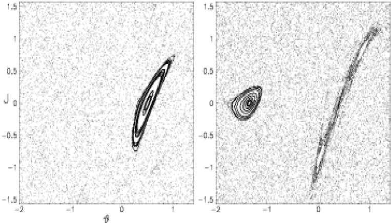
Figure 2: Same as Fig.1, for $\eta/\tau=0.01579$, ${\tilde{k}}=0.8\pi(4\pi-\tau)$, and different values of $\tau$. Left: at $\tau=10.996$, one stable fixed point exists with period $1$, ${\mathfrak{j}}=0$. On decreasing $\tau$ it turns unstable at $\tau\approx 10.813$, generating a period-2 stable orbit. At $\tau\approx 10.801$, one stable orbit with period $1$, ${\mathfrak{j}}=-1$ appears. Both orbits are shown in the phase portrait on the right, drawn at $\tau=10.744$.

Figure 3: Phase portraits for the $\epsilon$-classical dynamics on the torus, showing a $(5,-2)$ periodic orbit at $\tau=12.472$, ${\tilde{k}}=0.8\pi(4\pi-\tau)$, $\eta=0.01579\tau$ (left) and a $(10,1)$ periodic orbit at $\tau=6.31$, ${\tilde{k}}=0.8\pi(\tau-2\pi)$, $\eta=0.01579\tau$ (right).

3.2.3 $\epsilon-$Classical Accelerator Modes.

Primitive periodic orbits of the toral maps yield families of accelerator orbits of the original dynamics (25), marked by linear average growth of momentum with time:

$$\theta_{{\mathfrak{p}}t}=\theta_{0}=\vartheta_{0}\;\mbox{\rm mod}(2\pi)\;\;,\;\;I_{t{\mathfrak{p}}}=I_{0}+a{\mathfrak{p}}t\;,$$ (32)

where

$$I_{0}={\cal J}_{0}\mp\pi l\mp\tau(\beta+\frac{\eta}{2})+2\pi m\;\;,\;\;a=\frac{2\pi{\mathfrak{j}}}{{\mathfrak{p}}}\mp\tau\eta\;.$$ (33)

with $m$ any integer, and ${\cal J}_{0},\vartheta_{0}$ a period-${\mathfrak{p}}$ fixed point. If such accelerator orbits are stable, then they are surrounded by islands of positive measure in phase space, also leading to ballistic (linear) average growth of momentum in time. These are named accelerator modes.

We shall classify accelerator modes according to their order ${\mathfrak{p}}$ and jumping index ${\mathfrak{j}}$. By a $({\mathfrak{p}},{\mathfrak{j}})$-accelerator mode we shall mean a mode, whose order and jumping index are given by the integers ${\mathfrak{p}},{\mathfrak{j}}$ respectively.

3.2.4 Quantum Accelerator Modes in Rotor Dynamics.

Initial physical momenta $n_{0}=|\epsilon|^{-1}I_{0}$ for $\epsilon-$classical accelerator modes are obtained from (33) for any $0\leq\beta<1$ :

$$n_{0}\;=\;\frac{2\pi m+{\cal J}_{0}}{|\epsilon|}-\frac{\pi l}{\epsilon}-\frac{\tau}{\epsilon}(\beta+\frac{\eta}{2})$$ (34)

If the stable islands associated with $\epsilon-$classical accelerator modes have a large area compared to $|\epsilon|$, then they support a large number of quantum states. Thus they may trap some of the rotor’s wave packet and give rise to quantum accelerator modes traveling in physical momentum space with speed $\sim a/|\epsilon|=-\tau\eta/\epsilon+2\pi{\mathfrak{j}}/({\mathfrak{p}}|\epsilon|)$. In order that such modes may be observed, the phase space distribution associated with the initial rotor state must significantly overlap the islands. Even in that case the modes will eventually decay due to quantum tunneling out of the classical islands.

This picture is confirmed by numerical simulations. Fig.4 shows the quantum phase-space evolution of a $\beta-$rotor started in a coherent state centered at the position of the $(1,0)$- accelerator mode generated by the fixed point shown in Fig.1 (left). The Husimi functions computed at subsequent times closely follow the motion of the $\epsilon-$classical mode.

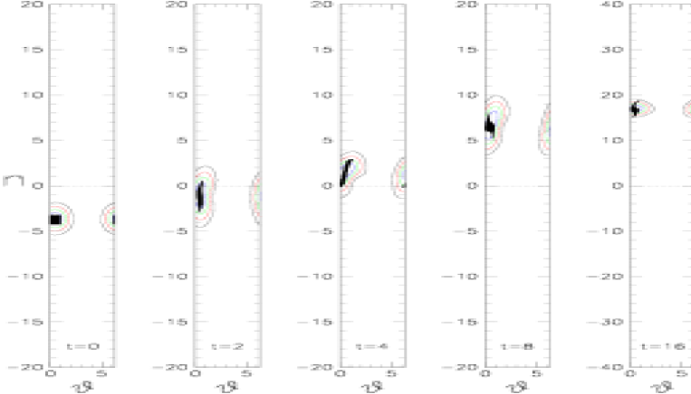
Figure 4: Quantum phase space evolution of the $\beta-$rotor with $\beta=0.218769$, ${\tilde{k}}=1.329$, $\tau=5.86$, $\eta=0.093$ initially prepared in the coherent state centered at the $\epsilon-$classical $(1,0)$ accelerator mode $n_{0}=-3.754$, $\theta_{0}=0.420$. Contour plots of the Husimi functions of the rotor are shown at times $t=$$0$,$2$,$4$,$8$,$16$. The black spots in the centers of the contours are an ensemble of classical phase points, initially distributed in a square of area $\hbar=1$ centered at the mode. They evolve according to the $\epsilon-$classical dynamics (25).

In Fig.5 we compare quantum and $\epsilon$-classical results after $30$ kicks, and different values of $\tau$ at fixed $k$ and $\eta/\tau$. In some of the examined $\tau$ range, two different $\epsilon$-classical modes are simultaneously present, with different signs of the acceleration. In order to single out one of them, we have plotted the quantities $E_{\pm}$, which, in the classical case, are equal to the average energy after $30$ kicks, computed over those rotors in the ensemble which, at the given time, have a positive (respectively, negative) momentum. In the quantum case, they are equal to the energy, computed in the state obtained by projecting the rotor state over the positive (respe., negative) momenta. The main peak in the left-hand plot is due to a $(1,0)$ mode whose interval of existence and stability is, according to (31), $1.043<\tau/(2\pi)<1.261$. Both the classical and the quantum data sharply arise at the onset of the mode. The rise of the quantum data is actually milder, because the $\epsilon$-classical island has to grow beyond a size $\sim\epsilon$ in order to be quantally significant (note that $|\epsilon|$ increases on increasing $\tau$). As the stability border is approached, the island starts shrinking again, the classical and the quantum mode become less and less effective; the latter somewhat faster, for the just mentioned reasons. At the stability border, a $(2,0)$ classical mode is originated by bifurcation, which is in fact signalled by a tiny peak in the classical data; however, no similar quantum structure is observed. The small peak on the leftmost part is an accelerator mode itself, see Sect. (3.2.6).

At not really small values of the “Planck’s constant” $\epsilon$, strong $\epsilon$-classical modes still leave quantal signatures. The quantum-classical correspondence turns however loose, in interesting ways. This is illustrated in the right hand part of Fig.5. Now $|\epsilon|$ decreases from left to right. The rightmost peak corresponds to a $(3,-1)$ mode (see Sect. 3.2.6), faithfully reproduced by quantum data. The main classical peak is the $(1,0)$ mode, active for $1.721<\tau/(2\pi)<1.862$. A significant quantum mode is also observed, with remarkable differences, however. In particular, the quantum mode has its maximum at the very point where the $(1,0)$ $\epsilon$-classical mode turns unstable, giving birth to a $(2,0)$ mode, as demonstrated in Fig.2 (right). Our explanation of this curious behaviour is as follows. When the stability island near a stable fixed points breaks at a bifurcation point, some remnants of its KAM structure nevertheless survive, in the form of broken tori (cantori). These provide but a partial barrier to classical motion, and allow for nonzero phase-area flux. If this flux is small compared to $\epsilon$, then the cantorus quantally acts as if it were unbroken [22] . Then it may give rise to a quantum accelerator mode, much more effectively than one might guess looking at the small area of stability of the bifurcated higher-period orbits.

Though $\epsilon-$classical modes exist at any value of $\beta$, their location in the $\beta$-rotor’s phase-space changes with $\beta$ . Hence their impact on the quantum evolution of a rotor state is enhanced at those values of $\beta$ which afford maximal overlap of the mode with the given state. In particular, if $\eta\tau<2\pi$, and the $\beta-$rotor is initially set in the $n=0$ momentum eigenstate, then the quantum $(1,0)$-accelerator modes are especially pronounced when $\beta=l\pi/\tau-\eta/2$. Note that $\beta$ was not set to this value in the case of of Fig.4.

Figure 5: Full dots: Quadratic spread $E_{\pm}(t)$ of the quantum $\beta$-rotor over positive (right) and negative (left) momenta after $30$ kicks, vs $\tau$, with $\eta/\tau=0.01579$, $k=0.8\pi$, $\beta=l\pi/\tau-\eta/2$, $l=1$ (left) and $l=2$ (right). The rotor was started at $n=0$. Full lines: same for an ensemble of $5\times 10^{6}$ classical rotors evolving according to (25), started with $n=0$ and $\theta$ uniformly distributed in $[0,2\pi]$. The exact meaning of $E_{\pm}(t)$ is explained in the text. At values of $\tau/2\pi\simeq 1.72$ the classical phase portraits are as shown in Fig.2.

In the $\epsilon-$ semiclassical regime, accelerator modes exponentially decay in time due to quantum tunneling out of the classical islands, with decay rate $\gamma_{\epsilon}\propto\exp{-(\mbox{\rm const.}/|\epsilon|)}$. The decay of quantum accelerator modes is numerically demonstrated in Fig.6.

Figure 6: Exponential decay of accelerator modes. Left: semilogarithmic plot of the probability $P_{\delta n}(t)$ in a moving momentum window of width $\delta n=15$ centered at the $\epsilon-$classical $(1,0)$ mode , versus time $t$, for $k=2.751$, $\tau=5.8$, $\epsilon=-0.483$, $\eta=0.092$, $\beta=\pi/\tau-\eta/2$. The asymptotic decay of $P_{\delta n}(t)$ is exponential with decay rate $\gamma_{\epsilon}\approx 0.32\times 10^{-4}$. Right: semilogarithmic plot of $\gamma_{\epsilon}$ vs $1/(|\epsilon|)$. The $\epsilon-$classical variables $\delta I=|\epsilon|\delta n$, ${\tilde{k}}=|\epsilon|k$ were held fixed at $7.540$, $1.329$ respectively while changing $\epsilon$. The fitting line corresponds to the law $\gamma_{\epsilon}\approx 135\times\exp(-7.35/|\epsilon|)$.

3.2.5 Quantum accelerator modes in Particle Dynamics.

Quantum Accelerator modes arise in the particle dynamics as well, just because such dynamics comes of a quantal superposition of $\beta-$rotors. We shall presently discuss the small-$\epsilon$ asymptotics of the particle dynamics. This will at once provide an alternative derivation of the $\epsilon$-classical rotor dynamics, and a means of translating into particle dynamics the results established in the previous sections.

Let us consider the propagator from state $|p\rangle$ to state $|x^{\prime}\rangle$ from (discrete) time $t$ to time $t+1$, for the particle dynamics (16). Let $p=n+\beta$ as usual, and $x^{\prime}=2m^{\prime}\pi+\theta^{\prime}$ with $m^{\prime}$ integer and $0\leq\theta^{\prime}<2\pi$. Then

$$\langle x^{\prime}|{\hat{U}}(t)|p\rangle = \frac{1}{\sqrt{2\pi}}\exp(i\phi(\beta,\theta^{\prime},t))$$ (35)

$$\times \exp\left(-ik\cos(\theta^{\prime})+in\theta^{\prime}+2im^{\prime}\pi\beta-\frac{i}{2}\epsilon n^{2}-in\pi l-in\tau(\beta+t\eta+\frac{\eta}{2})\right)\;,$$

where $e^{i\pi ln^{2}}=e^{i\pi ln}$ was used, and

$$\phi(\beta,\theta^{\prime},t)=\beta\theta^{\prime}-\frac{\tau}{2}\left(\beta+t\eta+\frac{\eta}{2}\right)^{2}\,.$$ (36)

Next we introduce $\epsilon$-classical scaled variables $I=n|\epsilon|$, ${\tilde{k}}=k|\epsilon|$, $L^{\prime}=-2\pi m^{\prime}|\epsilon|$, to be kept constant in the $\epsilon$-classical limit. Then (35) rewrites as:

$$\frac{1}{\sqrt{2\pi}}\,e^{i\phi(\beta,\theta^{\prime},t)}\,e^{\frac{i}{|\epsilon|}{\mathcal{F}}(\theta^{\prime},L^{\prime},\beta,I,t)},$$ (37)

where:

$${\mathcal{F}}(\theta^{\prime},L^{\prime},\beta,I,t)=I\theta^{\prime}-L^{\prime}\beta-{\tilde{k}}\cos(\theta^{\prime})-\frac{1}{2}\mbox{\rm sign}(\epsilon)I^{2}-I\left(\pi l+\tau(\beta+t\eta+\eta/2)\right)\,.$$ (38)

Considering $|\epsilon|$ as the Planck’s constant, and $I,L^{\prime}$ as canonical momenta respectively conjugated to $\theta,\beta^{\prime}$, the function ${\mathcal{F}}$ is a generating function for the canonical transformation $(\theta,I,\beta,L)\to(\theta^{\prime},I^{\prime},\beta^{\prime},L^{\prime})$ given by:

$$\beta^{\prime}\, = \,-\frac{\partial{\mathcal{F}}}{\partial L^{\prime}}\,=\,\beta$$

$$L\, = \,-\frac{\partial{\mathcal{F}}}{\partial\beta}\,=\,L^{\prime}+\tau I$$

$$I^{\prime}\, = \,\frac{\partial{\mathcal{F}}}{\partial\theta^{\prime}}\,=\,I+{\tilde{k}}\sin(\theta^{\prime})$$

$$\theta\, = \,\frac{\partial{\mathcal{F}}}{\partial I}\,=\,\theta^{\prime}-\mbox{\rm sign}(\epsilon)I-\pi l-\tau(\beta+t\eta+\eta/2)\;.$$ (39)

The second exponential in (37) is thus (apart from a constant prefactor) the $\epsilon$-semiclassical propagator associated with the $\epsilon$-classical map (3.2.5). The 3d and the 4th equation are just the $\epsilon$-classical $\beta$-rotor dynamics. The first equation says that quasi-momentum is conserved, and the second yields the complete revolutions accumulated by the $\beta$-rotor from time $t$ to $t+1$; this quantity is formally conjugated to quasi-momentum.

However, (37) has the additional phase factor $e^{i\phi}$, which is not $\epsilon$-semiclassical, because $\phi$ is not scaled by $|\epsilon|^{-1}$. While this factor is irrelevant for the fixed $\beta$ dynamics (and was in fact disregarded in sect. (3.2.1)), it cannot be neglected when studying the particle wavepacket dynamics, which requires integration over all values of $\beta$. Such integration causes $\epsilon$-classical trajectories of different $\beta$-rotors to interfere. This interference is ruled by the true Planck’s constant $\hbar=1$, and cannot be suppressed by the $\epsilon\to 0$ limit. Unlike the $\beta$-rotor dynamics, the particle dynamics does not become “classical” in the $\epsilon\to 0$ limit.

As long as $\beta$ is fixed, the maps (3.2.5) yield, in the physical variables $p,x$ and at $|p|,|x|>>1$:

$$p_{t} = |\epsilon|^{-1}I_{t}+\beta\sim p_{0}+\left(\frac{2\pi{\mathfrak{j}}}{{\mathfrak{p}}}\mp\tau\eta\right)\frac{t}{|\epsilon|}\;,$$

$$x_{t} \sim -|\epsilon|^{-1}L_{t}\sim x_{0}+n_{0}\tau\,t+\left(\frac{2\pi{\mathfrak{j}}}{{\mathfrak{p}}}\mp\tau\eta\right)\frac{\tau t(t-1)}{2|\epsilon|}$$ (40)

for a $({\mathfrak{p}},{\mathfrak{j}})$- accelerator mode (32) started at $x_{0}$, $p_{0}$.

Fig.7 shows the quantum evolution of a particle started at $t=0$ in the coherent state centered at the $(1,0)$-accelerator mode $p_{0}=0$, $x_{0}=0.42$. The phase-space distribution splits, the righmost part of it moving with constant acceleration $-\tau\eta/\epsilon$. This is the effect of the accelerator mode.

A conceptually simpler situation is met when the initial state of the particle is an incoherent mixture of plane waves, for in that case no interference occurs between different $\beta-$rotors. Let the initial particle state be described in the falling frame by the statistical operator:

$${\hat{\rho}}(0)\;=\;\int dp\;f(p)|p\rangle\langle p|\;,\;\;f(p)\geq 0\;,\;\int dp\;f(p)=1\;.$$ (41)

Each plane wave has a well-defined quasi-momentum, so it is equivalent to a unique $\beta-$rotor in the angular momentum eigenstate specified by the integer part of the momentum of the wave. Therefore, the statistical ensemble (41) is equivalent to a statistical ensemble of $\beta$-rotors. At any given quasi-momentum $\beta$, the state of the rotor is described by the statistical operator ${\hat{\rho}}_{\beta}=(P(\beta))^{-1}\sum_{n}f(n+\beta)|n\rangle\langle n|$; the distribution of quasi-momenta is further given by $P(\beta)=\sum_{n}f(n+\beta)$. The momentum distribution for the particle is given at time $t$ by

$$f(p,t)=P(\beta)\langle n|{\hat{\rho}}_{\beta}(t)|n\rangle\;$$ (42)

where $\beta=\{p\}$, $n=[p]$, and ${\hat{\rho}}_{\beta}(t)$ evolves according to the $\beta$-rotor dynamics (20). The distribution in momentum is then $\epsilon$-quasi classically that of an ensemble of classical rotors evolving according to (25).

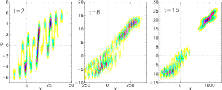
Figure 7: Quantum phase space evolution for a particle initially prepared in the coherent state centered at $p_{0}=0$, $x_{0}=0.42$, with $k=\pi$, $\tau=5.86$, $\eta=0.093$. The computation implements the Bloch-Wannier fibration discretized over $512$ values of quasi-momentum. Shades-of-grey plots of the Husimi function of the particle at times $t=2,8,16$ are shown.

3.2.6 Spectroscopy of accelerator modes.

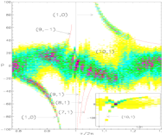
Figure 8: Momentum distribution in the falling frame after $60$ kicks for different values of the kicking period $\tau$ near $\tau=2\pi$, and for $k=0.8\pi$, $\eta=0.01579\tau$. Note the negative sign of $p$. Darker regions correspond to higher probability. The initial state is a mixture of $50$ plane waves sampled from a gaussian distribution of momenta. Full lines are the theoretical curves (43); they are drawn piecewise, to avoid hiding the actual structures to which they correspond. Their order and jumping index are indicated by the arrows. The inset shows data at $t=400$.

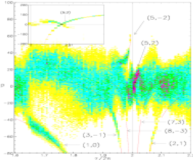
Figure 9: Same as Fig.8, for $\tau$ near $4\pi$. The inset shows data at time $t=400$.

In the experiments described in refs.[17, 18, 19], the initial state of the falling atoms is satisfactorily described, according to the same references, by (41), with $f(p)$ a Gaussian of rms deviation $\simeq 2.55$ (in our units) centered at $p=0$. In Figs. 8 and 9 we show numerical results obtained with the same choice of the initial state. Such results provide further evidence of accelerator modes, including higher order ones, which were not previously identified. The Figures were produced by computing the evolution of an ensemble of $50$ rotors with the mentioned initial distribution over $60$ kicks, for different values of the period $\tau$ near the main resonances $\tau=2\pi$, $\tau=4\pi$, and $k=0.8\pi$. As $\eta/\tau$ was kept fixed at the physical value $0.01579$, $\eta$ also varied with $\tau$. Fig.8 is analogous to the experimentally obtained Fig.2 in ref. [17] (with some differences in units and in parameter values, though).

The final distribution of momenta is represented by shades of grey in the $(p,\tau)$ plane, darker zones corresponding to higher probability. The hyperbolic-like structures near $\tau=2\pi,4\pi$ are signatures of quantum accelerator modes. At any $\tau$ where they are visible, they are in fact located at the momentum values reached at $t=60$ by certain accelerator modes, started at $t=0$ with $n_{0}\simeq 0$. Such values are theoretically predicted by eqs.(32). The $\epsilon$-classical $({\mathfrak{p}},{\mathfrak{j}})$-mode started at $t=0$ with $I_{0}=n_{0}|\epsilon|$ is located at time $t$ at the momentum:

$$n\simeq n_{0}-t\frac{\tau\eta}{\epsilon}+t\frac{2\pi{\mathfrak{j}}}{{\mathfrak{p}}|\epsilon|}\;.$$ (43)

Replacing $\epsilon=\tau-2\pi l$ ($l=1,2$ for Fig.8 and Fig.9 respectively), and $\eta=0.01579\tau$, one obtains a curve $n=n(\tau)$ for any chosen time $t$ and for any chosen $n_{0},{\mathfrak{p}},{\mathfrak{j}}$. Such curve is then observable, if a mode with the chosen ${\mathfrak{p}}$,${\mathfrak{j}}$ exists, which significantly overlaps the initial distribution. The narrow distribution of initial momenta legitimates the choice $n_{0}=0$; although other small values of $n_{0}$ are involved, they just result in a thickening of the curves.

Well-marked (1,0) modes are observed in both Figures. The intervals of existence and stability of the $\epsilon$-classical $(1,0)$ modes predicted by (31) are $0.745<\tau/(2\pi)<0.963$ and $1.043<\tau/(2\pi)<1.261$ for the case of Fig.8. The $(1,0)$ mode in Fig.9 is the same as in Fig.5; in most of its range the $\epsilon$-classical structure is like the one shown in Figs.2 and 5. It has both a $(1,-1)$ stable orbit and a $(2,0)$ stable orbit originated by bifurcation. The $(1,-1)$ theoretical curve mostly lies at negative values of $p$ off the scale of the figure, and no significant trace of it was detected in our quantum computation, indicating that the island was too tiny compared to the relatively large values of $|\epsilon|$. We therefore explain the large $(1,0)$ structure obaserved by the same quantal mechanism discussed in sect. (3.2.4), namely localization by cantori.

Higher-order modes $(10,\pm 1)$ and $(5,\pm 2)$ are observed close to $\tau=2\pi$ and $\tau=4\pi$ respectively. The corresponding $\epsilon$-classical modes are shown in Fig.3. The small, yet well marked, structure produced by the $(10,1)$ mode near $2\pi$ is also visible in experimental data in [17]. The correspondence of the $(5,2)$- and $(10,1)$-modes with the curves (43) is remarkably evident at longer times, see the insets in Figs.8 and 9.

In Figs.8 and 9 other higher-order modes are visible, too. These were identified by first fitting the observed structure with a curve (43), and then checking that the $\epsilon$-classical phase space really displays, in the relevant $\tau$ range, a stable orbit with the found ${\mathfrak{p}},{\mathfrak{j}}$. A few of these left but a dim trace in Figs.8 and 9. This may be due on one hand to mutual interference of different modes when they coexist in the same $\tau$-range, and on the other hand to the small number of rotors used in the computation. For such reasons, Figs.8 and 9 do not probably account for all the accelerator modes which are excited in their respective parameter ranges.

Generally speaking, the family of higher-order modes that are potentially observable in Figures like 8 and 9 (and in experiments as well) is probably much richer than shown here. These might be exposed by varying parameters, and also by a fine scan of smaller $\epsilon$ ranges. It looks likely that momentum distributions at relatively short times, of the type shown in Figs.8 and 9, can be altogether described by accelerator mode spectroscopy, i.e identification of accelerator modes and analysis of their mutual interference. Such a systematic analysis is beyond the scope of this work.

4 Concluding remarks.

1) The above theory of accelerator modes hinges on reduction to independent kicked rotors models, wherein such modes admit a natural interpretation in terms of classical trajectories. It is the conservation of quasi-momentum that allows for such reduction. Accelerator modes in particle dynamics are a purely quantal effect, in fact a remarkable manifestation of the conservation of quasi-momentum (in the falling frame).

2) The fact that the intermediate-time dynamics is dominated by a discrete set of modes, which exponentially decay in time, bears a distinct resemblance to the Wannier-Stark problem of a Bloch particle in a constant field [23]. How far this analogy carries is, in our opinion, a very interesting question.

3) The time-dependent variants of the Kicked Rotor model examined in this paper also raise other important theoretical questions, which were not addressed in this paper. These are about the long-time asymptotics of the dynamics, and the localization-delocalization issue in particular.

4) In the experiments [17, 18, 19] the initially prepared states form an incoherent superposition of momentum eigenstates, and of quasimomentum states. Therefore the results of the of the calculations for the $\beta$-rotors explain the experiments. The particle nature (compared to the rotor) is important only for initial coherent superpositions of momentum eigenstates. It will of great interest if this point is explored experimentally.

5 Appendix: Resonances in the presence of Gravity

In this appendix we assume $\tau=2\pi l$, with $l\neq 0$ integer. We denote $\psi(x)=\langle x|\psi\rangle$ the wave function of the particle in the position representation, and ${\mathcal{E}}(t)$ the kinetic energy at time $t$ (in the falling frame).

Proposition: Let $\int dx\;|x|^{2\alpha}|\psi(x)|^{2}<+\infty$ for some $\alpha>1$. Then:

(I) If $\eta=0$ :

$${\mathcal{E}}(t)={\mathcal{E}}(0)+\frac{k^{2}Dt}{4}\;+\;O(t^{\lambda})\;,\;\;\;\;\lambda=\mbox{\rm\small max}\{2-\alpha,\frac{1}{2}\}$$

where:

$$D\;=\;\frac{1}{l}\sum\limits_{n=0}^{l-1}\int_{0}^{2\pi}d\theta|\langle\theta|\Psi_{\beta_{n}}\rangle|^{2}\;\;,\;\;\beta_{n}=\frac{n}{l}+\frac{l}{2}\;\mbox{\rm mod}(1)\;.$$ (44)

(II) If $\eta\neq 0$ satisfies a Diophantine condition, that is, there are constants $c,\gamma>0$ so that for all integer $p,q$ :

$$\left|\eta-\frac{p}{q}\right|\;\geq\;c\;q^{-2-\gamma}\;$$ (45)

then:

$${\mathcal{E}}(t)={\mathcal{E}}(0)+\frac{k^{2}t}{4}+O(t^{\sigma})\;,\;\;\;\;\sigma=\mbox{\rm\small max}\{2-\alpha+\gamma,\frac{1}{2})$$ (46)

Remarks:

1. The quasi-momenta $\beta_{n}$’s in part (I) are exactly those yielding quadratic growth of the $\beta-$rotor energy.

2. Part (II) ensures that, for all $\eta$ in a set of full measure, the energy grows diffusively with coefficient $k^{2}/4$.

Proof: Numerical constants will share the common notation $C$ whenever their exact value is irrelevant. From (21),

$$\langle n|{\hat{\mathcal{R}}}_{\beta}(t)|\Psi_{\beta}(t)\rangle\;=\;e^{-i\pi ln(1+2\beta+2t\eta+\eta)}e^{i\phi(\beta,\eta,t)}\langle n|\Psi_{\beta}(t)\rangle\;$$

The explicit form of the phase $\phi$ is not important for our present purposes. Further,

$$\langle\theta|\Psi_{\beta}(t+1)\rangle\;=\langle\theta|{\hat{\mathcal{K}}}{\hat{\mathcal{R}}}_{\beta}(t)|\Psi_{\beta}(t)\rangle\;=\;e^{i\phi(\beta,\eta,t)}e^{-ik\cos(\theta)}\langle\theta-a-bt|\Psi_{\beta}(t)\rangle\;,$$

where:

$$a\;=\;\pi l(1+2\beta+\eta)\;\;,\;\;b=2\pi l\eta\;.$$ (47)

It follows that:

$$\langle\theta|\Psi_{\beta}(t)\rangle\;=\;e^{-i\phi(\beta,\eta,t)}e^{-ikF(\theta,\beta,t)}\langle\theta-at-\frac{b}{2}t(t-1)|\Psi_{\beta}(0)\rangle$$

where:

$$F(\theta,\beta,t)\;=\;\sum\limits_{r=0}^{t-1}\cos(\theta-ra-rbt+r^{2}b/2+rb/2)$$

We now use eqn.(14). As already remarked, the dominant contribution is given by the 1st term on the rhs, corrections being on the order of square root of that term. We hence restrict to that term. After substituting the above equations, it takes the form:

$$\frac{1}{2}\int_{0}^{1}d\beta\int_{0}^{2\pi}d\theta\;\left|\frac{d}{d\theta}\langle\theta|\Psi_{\beta}(t)\rangle\right|^{2}={\mathcal{E}}_{0}(t)+{\mathcal{E}}_{1}(t)+{\mathcal{E}}_{2}(t),$$ (48)

having denoted

$$\begin{array}[]{ccc}{\mathcal{E}}_{0}(t)&=&\frac{1}{2}\int_{0}^{1}d\beta\int_{0}^{2\pi}d\theta|g^{\prime}(\theta,t)|^{2}\;,\\ {\mathcal{E}}_{1}(t)&=&\frac{k^{2}}{2}\int_{0}^{1}d\beta\int_{0}^{2\pi}d\theta F^{{}^{\prime}2}(\theta,\beta,t)|g(\theta,t)|^{2}\;,\\ {\mathcal{E}}_{2}(t)&=&k\;\Re\int_{0}^{1}d\beta\int_{0}^{2\pi}d\theta\;iF^{\prime}(\theta,\beta,t)g^{*}(\theta,t)g^{\prime}(\theta,t)\\ g(\theta,t)&=&\langle\theta-ta-bt^{2}/2+bt/2|\Psi_{\beta}(0)\rangle\end{array}$$

(primes denote differentiation with respect to $\theta$). An obvious shift in $\theta$ shows that

$${\mathcal{E}}_{0}(t)=\mbox{\rm const}={\mathcal{E}}_{0}(0).$$ (49)

Moreover, from the Cauchy-Schwarz inequality it follows that:

$$|{\mathcal{E}}_{2}(t)| \leq k\left(\int_{0}^{1}d\beta\int_{0}^{2\pi}d\theta F^{{}^{\prime}2}(\theta,\beta,t)|g(\theta,t)|^{2}\right)^{1/2}\left(\int_{0}^{1}d\beta\int_{0}^{2\pi}d\theta|g^{\prime}(\theta,t)|^{2}\right)^{1/2}$$ (50)

$$= 2{\mathcal{E}}_{1}(t)^{1/2}\;{\mathcal{E}}_{0}(0)^{1/2}$$

The dominant contribution to ${\mathcal{E}}(t)$ is thus given by ${\mathcal{E}}_{1}(t)$, so ${\mathcal{E}}_{0}$, ${\mathcal{E}}_{2}$ will not be considered until the end of the proof. After an obvious change of variables,

$${\mathcal{E}}_{1}(t)\;=\;\frac{k^{2}}{2}\int_{0}^{1}d\beta\int_{0}^{2\pi}d\theta\left(\sum\limits_{r=1}^{t}\sin(\theta+ra+br^{2}/2-br/2)\right)^{2}|\langle\theta|\Psi_{\beta}(0)\rangle|^{2}\;.$$ (51)

We rewrite the square of the sum as a double sum, then apply standard trigonometric formulae, and finally replace $a,b$ by (47), leading to :

$${\mathcal{E}}_{1}(t)\;=\;\frac{k^{2}}{2}\int_{0}^{1}d\beta\int_{0}^{2\pi}d\theta\;|\langle\theta|\Psi_{\beta}(0)\rangle|^{2}\;\left(A_{1}(\beta,t)-A_{2}(\beta,\theta,t)\right)$$ (52)

with

$$\begin{array}[]{ccc}A_{1}(\beta,t)&=&\frac{1}{2}\sum\limits_{r,s=1}^{t}(-)^{(r+s)l}\cos\left(2\pi l\beta(r-s)+\pi l\eta(r^{2}-s^{2})\right)\;,\\ A_{2}(\beta,\theta,t)&=&\frac{1}{2}\sum\limits_{r,s=1}^{t}(-)^{(r+s)l}\cos\left(2\theta+2\pi\beta(r+s)+\pi l\eta(r^{2}+s^{2})\right)\;.\end{array}$$

Now we expand $|\langle\theta|\Psi_{\beta}(0)\rangle|^{2}$ in Fourier series:

$$|\langle\theta|\Psi_{\beta}(0)\rangle|^{2}\;=\;\sum\limits_{M,N}\;c(M,N)\;e^{2\pi iM\beta}\;e^{iN\theta}\;$$ (53)

Replacing in (52) we obtain

$${\mathcal{E}}_{1}(t)\;=\;\frac{1}{2}\pi k^{2}\Re(B_{1}-B_{2})\;,$$ (54)

where:

$$B_{1}\; = \;\sum\limits_{r,s=1}^{t}c(l(r-s),0)(-)^{(r-s)l}e^{-i\pi l\eta(r^{2}-s^{2})}$$

$$= \;\sum\limits_{j=1-t}^{t-1}c(lj,0)(-)^{lj}e^{i\pi l\eta j^{2}}\sum\limits_{r=\mbox{\rm\small max}(1,j+1)}^{\mbox{\rm\small min}(t,j+t)}e^{-2\pi il\eta rj}\;,$$

$$B_{2}\; = \;\sum\limits_{r,s=1}^{t}c(l(r+s),2)(-)^{l(r+s)}e^{-i\pi l\eta(r^{2}+s^{2})}$$ (56)

$$= \;\sum\limits_{j=2}^{2t}c(lj,2)(-)^{lj}e^{-i\pi l\eta j^{2}}\sum\limits_{r=\mbox{\rm\small max}(1,j-t)}^{\mbox{\rm\small min}(t,j-1)}e^{-2\pi il\eta r(r-j)}\;.$$

With the help of the Lemma proven in the end of this section, $B_{2}$ is bounded by :

$$\sum\limits_{j=2}^{1+t}|c(lj,2)|(j-1)+\sum\limits_{j=t+2}^{2t}|c(lj,2)|(2t-j+1)\leq C\sum\limits_{j=2}^{2t}(j-1)j^{-\alpha}+Ct\sum\limits_{j=t+2}^{2t}j^{-\alpha}\;=\;O(t^{2-\alpha})\;.$$

Here and in the following $O(t^{x})$ has to be read as $O(\log t)$, $O(1)$ whenever $x=0$, $x<0$ respectively. In order to estimate $B_{1}$ we distinguish two cases;

Case I: $\eta=0$.

$$B_{1}\;=\;\sum\limits_{j=1-t}^{t-1}c(lj,0)(-)^{lj}(t-|j|) = t\sum\limits_{j=-\infty}^{\infty}(-)^{lj}c(lj,0)+O(t^{2-\alpha})$$ (57)

$$= \frac{Dt}{2\pi}+O(t^{2-\alpha})$$

where

$$D\; = \;2\pi\sum\limits_{j=-\infty}^{\infty}(-)^{lj}c(lj,0)$$ (58)

$$= \;\frac{2\pi}{l}\sum\limits_{n=0}^{l-1}\sum\limits_{j^{\prime}=-\infty}^{\infty}c(j^{\prime},0)e^{\pi ij^{\prime}(2n/l+l)}\;$$

$$= \;\frac{1}{l}\sum\limits_{n=0}^{l-1}\int_{0}^{2\pi}d\theta|\langle\theta|\Psi_{\beta_{n}}\rangle|^{2}\;\;,\;\;\beta_{n}=\frac{n}{l}+\frac{l}{2}\;\mbox{\rm mod}\;(1)\;.$$

We next substitute (57) and (58) in (54), and then in (48). Recalling (49),(50), and the remark preceding (48) leads to (44).

Case II: $\eta$ a Diophantine irrational. The sum (5) is written in the form

$$B_{1}\;=\;c(0,0)t+S$$

where $S$ is the contribution of all $j\neq 0$ terms. It can be bounded as

$$|S|\; \leq \;2\sum\limits_{j=1}^{t-1}|c(jl,0)|\frac{2}{|\sin(\pi l\eta j)|}$$ (59)

$$\leq \;C\sum\limits_{j=1}^{t-1}|c(jl,0)|j^{1+\gamma}\;=\;O(t^{2-\alpha+\gamma}).$$

where (45) was used. The normalization of the wavefunction implies $c(0,0)=1/(2\pi)$. Substituting in (54) leads to (46) after the same concluding steps as in Case I above. This completes the proof. $\Box$

Lemma. Under the hypotheses of the Proposition, and with $c(M,N)$ defined as in (53), $|c(M,N)|=O(|M|^{-\alpha})$ as $M\to\infty$.

Proof. From the Bloch-Wannier fibration (8) it follows that, if $|M|\geq 1$, then:

$$|c(M,N)| = \frac{1}{2\pi}\left|\int dx\;\psi^{*}(x+M\pi)\psi(x-M\pi)\;e^{-iNx}\right|$$ (60)

$$\leq C|M|^{-\alpha}\int dx\;|\psi^{*}(x+M\pi)\psi(x-M\pi)|Q(x,M)\;$$

where $Q(x,M)=(1+(x+M\pi)^{2})^{\alpha/2}(1+(x-M\pi)^{2})^{\alpha/2}\geq(4\pi^{2}M^{2})^{\alpha/2}$. The Cauchy-Schwarz inequality then yields :

$$|c(M,N)|\leq C|M|^{-\alpha}\int dx\;|\psi(x)|^{2}\;(1+x^{2})^{\alpha}<\infty\;,$$

as the convergence of the integral was assumed in the Proposition. $\Box$

Acknowledgments. This research was supported in part by PRIN-2000: Chaos and localisation in classical and quantum mechanics, by the US-Israel Binational Science Foundation (BSF), by the US National Science Foundation under Grant No. PHY99-07949, by the Minerva Center of Nonlinear Physics of Complex Systems, by the Max Planck Institute for the Physics of Complex Systems in Dresden, and by the fund for Promotion of Research at the Technion. Useful discussions with M. Raizen, M. Oberhaler and Y. Gefen are acknowledged.

References

- [1] for reviews see, e.g.: F.M. Izrailev, Phys. Rep. 196, 299 (1991); S. Fishman, in Proceedings of the International School of Physics Enrico Fermi: Varenna Course CXIX, G.Casati, I. Guarneri and U.Smilansky eds., North Holland 1993, p.187.
- [2] B.V.Chirikov, Phys.Rep. 52, 263 (1979).
- [3] A.J. Lichtenterg and M.A. Liberman, Regular and Chaotic Dynamics, (Springer-Verlag, NY, 1992)
- [4] G.M. Zaslavsky, M. Edelman, and B.A. Niyazov, Chaos 7, 159 (1997); G. M. Zaslavsky and M. Edelman, Chaos 10, 135 (2000).
- [5] S. Fishman, D.R. Grempel, and R.E. Prange, Phys. Rev. Lett. 49, 509 (1982); D.R. Grempel, R.E. Prange, and S. Fishman, Phys. Rev. A 29, 1639 (1984).
- [6] J.D. Hanson, E. Ott, and T.M. Antonsen, Phys. Rev. A 29, 819 (1984); A. Iomin, S. Fishman and G. Zaslavsky, to be published in Phys. Rev. E.
- [7] F.M.Izrailev and D.L.Shepelyansky, Sov. Phys. Dokl. 24, 996 (1979); G.Casati and I.Guarneri, Comm. Math. Phys. 95, 121 (1984).
- [8] G.Casati, B.V. Chirikov, D.L. Shepelyansky, and I.Guarneri, Phys. Rep. 154, 2 (1987); G.Casati, I.Guarneri and D.L.Shepelyansky, IEEE J. Quantum. Electron. 24, 1420 (1988), and references therein.
- [9] E.J.Galvez, J.E.Sauer, L.Moorman, P.M..Koch, and D.Richards, Phys. Rev. Lett. 61, 2011 (1988); J.E.Bayfield, G.Casati, I.Guarneri, and D.W.Sokol, Phys. Rev. Lett. 63, 364 (1989); M.Arndt, A.Buchleitner, R.N.Mantegna, and H.Walther, Phys. Rev. Lett. 67, 2435 (1991).
- [10] D.A. Steck, V. Milner, W.H. Oskay, and M.G. Raizen, Phys. Rev. E 62, 3461 (2000); F. L. Moore, J. C. Robinson, C. F. Bharucha, Bala Sundaram, and M. G. Raizen, Phys. Rev. Lett. 75, 4598 (1995); C. F. Bharucha, J. C. Robinson, F. L. Moore, Qian Niu, Bala Sundaram, and M. G. Raizen, Phys. Rev. E 60, 3881 (1999); B.G. Klappauf, W.H. Oskay, D.A. Steck amd M.G. Raizen, Physica (Amsterdam) 131 D, 78 (1999).
- [11] R. Graham, M. Schlautmann and P. Zoller, Phys. Rev. A 45, R19 (1992).
- [12] , C.Cohen-Tannoudji and J.Dupont-Roc, Atom-Photon interactions: basic processes and applications, Gilbert Grynberg 1992.
- [13] R. Blumel, S. Fishman and U. Smilansky, J. Chem. Phys. 84, 2604-2614 (1986).
- [14] F.M. Izrailev, Phys. Rev. Lett. 56, 541 (1986).
- [15] W. H. Oskay, D. A. Steck, V. Milner, B. G. Klappauf, and M. G. Raizen, Opt. Comm. 179, 137 (2000).
- [16] S.Wimberger, I.Guarneri and S.Fishman, in preparation.
- [17] M.K. Oberthaler, R.M.Godun, M.B. d’Arcy, G.S. Summy, and K. Burnett, Phys. Rev. Lett. 83, 4447 (1999).
- [18] R.M.Godun, M.B. d’Arcy, M.K. Oberthaler, G.S. Summy, and K. Burnett, Phys. Rev. A62, 013411 (2000).
- [19] M.B. d’Arcy, R.M.Godun, M.K. Oberthaler, G.S. Summy, and K. Burnett, S.A. Gardiner, Phys. Rev. E 64, 056233 (2001)
- [20] D.L. Shepelyansky, Physica D8 208 (1983); G. Casati, G.Mantica and D.L.Shepelyansky, Phys. Rev. E63 066217 (2001), and references therein.
- [21] L.D. Landau and E.M. Lifshiz, Quantum Mechanics, 3d edition (Pergamon, Oxford 1977), p.76.
- [22] T. Geisel, G.Radons and J.Rubner, Phys. Rev. Lett. 57, 2883 (1986); R.S. MacKay and J.D. Meiss, Phys. Rev. A37, 4702 ( 1988); J.D. Meiss, Phys. Rev. Lett. 62, 1576 (1989); D.R. Grempel, S. Fishman and R.E. Prange, Phys. Rev. Lett. 53, 1212 (1984); S. Fishman, D.R. Grempel and R.E. Prange, Phys. Rev. A 36, 289 (1987).
- [23] for a review see, e.g., G. Nenciu, Rev. Mod. Phys. 63, 91 (1993) and references therein.
- [24] S. Fishman, D.R. Grempel and R.E. Prange, Phys. Rev. A36, 289-305 (1987).