Understanding deterministic diffusion by correlated random walks

Abstract

Low-dimensional periodic arrays of scatterers with a moving point particle are ideal models for studying deterministic diffusion. For such systems the diffusion coefficient is typically an irregular function under variation of a control parameter. Here we propose a systematic scheme of how to approximate deterministic diffusion coefficients of this kind in terms of correlated random walks. We apply this approach to two simple examples which are a one-dimensional map on the line and the periodic Lorentz gas. Starting from suitable Green-Kubo formulas we evaluate hierarchies of approximations for their parameter-dependent diffusion coefficients. These approximations converge exactly yielding a straightforward interpretation of the structure of these irregular diffusion coeficients in terms of dynamical correlations.

PACS numbers: 05.45.Ac,05.60.Cd,05.10.-a,05.45.Pq,02.50.Ga

I Introduction

Deterministic diffusion is a prominent topic in the theory of chaotic dynamical systems and in nonequilibrium statistical mechanics [1, 2]. To achieve a proper understanding of the mechanism of deterministic diffusion with respect to microscopic chaos in the equations of motion, a number of simple model systems was proposed and analyzed. An interesting finding was that, for a simple one-dimensional chaotic map on the line, the diffusion coefficient is a fractal function of a control parameter [3, 4, 5]. Diffusion coefficients exhibiting similar irregularities are also known for more complicated sytems such as sawtooth maps [6], standard maps [7], and Harper maps [8], the latter two models being closely related to physical systems like the kicked rotor, or a particle moving in a periodic potential under the influence of electric and magnetic fields. More recently, related irregularities in the diffusion coefficient were discovered in Hamiltonian billiards such as the periodic Lorentz gas [9], and for a particle moving on a corrugated floor under the influence of an external field [10]. That this phenomenon is not specific to diffusion coefficients is suggested by results on other transport coefficients such as chemical reaction rates in multibaker maps [11], electrical conductivities in the driven periodic Lorentz gas [12], and magnetoresistances in antidot lattices [13] which, again, exhibit strongly irregular behavior under parameter variation.

In this paper we wish to contribute to the further analysis and understanding of irregular transport coefficients in simple model systems. We use certain forms of the Green-Kubo formula as starting points for expansions of the diffusion coefficient in terms of correlated random walks. In Section 2 we exemplify this approach for the piecewise linear map on the line studied in Refs. [3, 4, 5]. In Section 3 we apply a suitably adapted version of it to diffusion in the periodic Lorentz gas. In both cases our approximations converge quickly to the precise diffusion coefficient as obtained from other numerical methods. We argue that for both models this approximation scheme provides a physical explanation for the irregular structure of these diffusion coefficients in terms of dynamical correlations, or memory effects. In Section 4 we summarize our results and relate them to previous work on irregular and fractal transport coefficients.

II Deterministic diffusion in one-dimensional maps on the line

Probably the most simple models exhibiting deterministic diffusion are one-dimensional maps defined by the equation of motion

$$x_{n+1}=M_{a}(x_{n})$$ (1)

where $a\in\hbox{\mb R}$ is a control parameter and $x_{n}$ is the position of a point particle at discrete time $n$. $M_{a}(x)$ is continued periodically beyond the interval $[0,1)$ onto the real line by a lift of degree one, $M_{a}(x+1)=M_{a}(x)+1$. We assume that $M_{a}(x)$ is anti-symmetric with respect to $x=0$, $M_{a}(x)=-M_{a}(-x)$. Let

$$m_{a}(x):=M_{a}(x)\quad\mbox{mod}\;1$$ (2)

be the reduced map related to $M_{a}(x)$. This map governs the dynamics on the unit interval according to $x_{n}=m_{a}^{n}(x)$. Let $\rho_{n}(x)$ be the probability density on the unit interval of an ensemble of moving particles starting at initial conditions $x\equiv x_{0}$. This density evolves according to the Frobenius-Perron continuity equation

$$\rho_{n+1}(x)=\int_{0}^{1}dy\>\rho_{n}(y)\>\delta(x-m_{a}(y))\quad.$$ (3)

Here we are interested in the deterministic diffusion coefficient defined by the Einstein formula

$$D(a)=\lim_{n\to\infty}<(x_{n}-x_{0})^{2}>/(2n)$$ (4)

with $x_{n}$ governed by $M_{a}(x)$, where the brackets denote an average over the initial values $x_{0}$ with respect to the invariant probability density on the unit interval, $\left\langle\ldots\right\rangle:=\int_{0}^{1}dx\;\rho_{a}^{*}(x)\ldots$. Eq.(4) can be transformed onto the Green-Kubo formula for maps [1, 4, 14, 15],

$$D(a)=\frac{1}{2}\left\langle j^{2}(x_{0})\right\rangle+\sum_{k=1}^{\infty}\left\langle j(x_{0})j(x_{k})\right\rangle\quad,$$ (5)

where the jump velocity

$$j(x_{n}):=[x_{n+1}]-[x_{n}]\quad,$$ (6)

$[x]$ being the largest integer less than $x$, takes only integer values and denotes how many unit intervals a particle has traversed after one iteration starting at $x_{n}$. The map we study as an example is defined by

$$M_{a}(x)=\left\{\begin{array}[]{r@{\quad,\quad}l}ax&0<x\leq\frac{1}{2}\\ ax+1-a&\frac{1}{2}<x\leq 1\end{array}\right\}\quad,$$ (7)

where the uniform slope $a>2$ serves as a control parameter. The Lyapunov exponent of this map is given by $\lambda(a)=\ln a$ implying that the dynamics is chaotic. A sketch of this map is shown in Fig. 1 (a). Fig. 1 furthermore depicts the parameter-dependent diffusion coefficient of this map in the regime of $2\leq a\leq 4$ as calculated in Refs. [3, 4, 5] by means of a numerical implementation of analytical methods. In these references numerical evidence was provided that the irregularities on a fine scale are reminiscent of an underlying fractal structure.

To analyze this fractal diffusion coefficient, Eq.(5) forms a suitable starting point because it distinguishes between two crucial contributions of the dynamics to the diffusion process, which are (1) the motion of the particle on the unit interval $x_{n}\;\mbox{mod}\;1$ generating the invariant density $\rho_{a}^{*}(x)$, and (2) the integer jumps from one unit interval to another one as related to $j(x_{n})$. In fact, in Refs. [4, 11] it was shown that both parts are independent sources of fractality for the diffusion coefficient. However, in these references Eq. (5) was only discussed in the limit of infinite time. In this paper we suggest to look at the contributions of the single terms in this expansion, and to analyze how the Green-Kubo formula approaches the exact diffusion coefficient step by step. We do this by systematically building up hierarchies of approximate diffusion coefficients. These approximations should be defined such that the different dynamical contributions to the diffusion process are properly filtered out. Another issue is how to evaluate the single terms of the Green-Kubo expansion on an analytical basis. In this section we show how to do this for the one-dimensional model introduced above, in the next section we apply the same idea to billiards such as the periodic Lorentz gas.

We start by looking at the first term in Eq.(5). For $a<4$ the absolute value of the jump velocity $j(x_{n})$ is either zero or one. Assuming that $\rho_{a}^{*}(x)\simeq 1$ for $a\to 2$ and cutting off all higher order-terms in Eq. (5), the first term leads to the well-known random walk approximation of the diffusion coefficient [4, 14, 16, 17, 18]

$$D_{0}(a)=\frac{1}{2}\int_{0}^{1}dx\;j^{2}_{a}(x)$$ (8)

which in case of the map Eq. (7) reads

$$D_{0}(a)=(a-2)/(2a)\quad.$$ (9)

This solution is asymptotically correct in the limit of $a\to 2$. More generally speaking, the reduction of the Green-Kubo formula to the first term only is an exact solution for arbitrary parameter values only if all higher-order contributions from the velocity autocorrelation function $C(n):=<j(x_{0})j(x_{n})>$ are strictly zero. This is only true for systems of Bernoulli type [14]. Conversely, the series expansion in form of Eq. (5) systematically gives access to higher-order corrections by including higher-order correlations, or memory effects. This leads us to the definition of two hierarchies of correlated random walk diffusion coefficients:

(1) Again, we make the approximation that $\rho_{a}^{*}(x)\simeq 1$. We then define

$$D_{n}^{j}(a):=\frac{1}{2}\int_{0}^{1}dx\;j^{2}(x)+\sum_{k=1}^{n}\int_{0}^{1}dx\;j(x)j(x_{k})\;,\;n>0\quad,$$ (10)

with $D_{0}(a)$ given by Eq. (8). Obviously, this series cannot converge to the exact $D(a)$.

(2) By using the exact invariant density in the averages of Eq.(5) we define

$$D_{n}^{\rho}(a):=\frac{1}{2}\int_{0}^{1}dx\;\rho_{a}^{*}(x)j^{2}_{a}(x)+\sum_{k=1}^{n}\int_{0}^{1}dx\;\rho_{a}^{*}(x)j_{a}(x)j_{a}(x_{k})\;,\;n>0\quad,$$ (11)

here with $D_{0}^{\rho}(a)=\frac{1}{2}\int_{0}^{1}dx\;\rho_{a}^{*}(x)j^{2}_{a}(x)$, which of course must converge exactly. The approximations $D_{n}^{j}(a)$ and $D_{n}^{\rho}(a)$ may be understood as time-dependent diffusion coefficients according to the Green-Kubo formula Eq. (5). According to their definitions, $D_{n}^{j}(a)$ enables us to look at contributions coming from $j(x_{n})$ only, whereas $D_{n}^{\rho}(a)$ assesses the importance of contributions resulting from $\rho_{a}^{*}(x)$. The rates of convergence of both approximations give an estimate of how important higher-order correlations are in the different parameter regions of the diffusion coefficient $D(a)$.

Similarly to Eq. (9), the next order $D_{1}(a)$ can easily be calculated analytically and reads

$$D_{1}(a)=\left\{\begin{array}[]{r@{\quad,\quad}l}(a-2)/(2a)&2<a\leq 1+\sqrt{3}\quad\mbox{and}\quad 2+\sqrt{2}<a\leq 4\\ 3/2-3/a-2/a^{2}&1+\sqrt{3}<a\leq 3\\ -1/2+3/a-2/a^{2}&3<a\leq 2+\sqrt{2}\end{array}\right\}\quad.$$ (12)

Further corrections up to order $n=3$ were obtained from computer simulations, that is, an ensemble of point particles was iterated numerically according to Eq. (1). All results are contained in Fig. 1 showing that this hierarchy of correlated random walks generates a self-affine structure which resembles, to some extent, the one of the well-known Koch curve. Fig. 1 (a) illustrates that this structure forms an important ingredience of the exact diffusion coefficient $D(a)$ thus explaining basic features of its fractality. Indeed, a suitable generalization of this approach in the limit of time to infinity leads to the formulation of $D(a)$ in terms of fractal generalized Takagi functions [4, 11].

Fig. 1 (b) depicts the results for the series of $D_{n}^{\rho}(a)$ up to order $n=2$ as obtained from computer simulations. This figure illustrates that there exists a second source for an irregular structure related to the integration over the invariant density, as was explained above. In the Green-Kubo formula Eq.(5) both contributions are intimately coupled with each other via the integration over phase space.

We now perform a more detailed analysis to reveal the precise origin of the hierarchy of peaks in Fig. 1. For this purpose we redefine Eq. (10) as

$$D_{n}^{j}(a)=\int_{0}^{1}dx\;j(x)J_{n}(x)-\frac{1}{2}\int_{0}^{1}dx\;j^{2}(x)\;,\;n>0\quad,$$ (13)

where we have introduced the jump velocity function

$$J_{n}(x):=\sum_{k=0}^{n}j(x_{k})\quad.$$ (14)

From Eq. (6) it follows $J_{n}(x)=[x_{n+1}]$, that is, this function gives the integer value of the displacement of a particle starting at some initial position $x$. In Fig. 2 we depict some representative results for $J_{1}(x)$ under variation of the control parameter $a$. Because of the symmetry of the map we restrict our considerations to $0<x<0.5$. Eq. (13) tells us that the product of this function with $j(x)$ determines the diffusion coefficient $D(a)$. The shaded bar in Fig. 2 marks the subinterval in which $j(x)=1$, whereas $j(x)=0$ otherwise, thus an integration over $J_{1}(x)$ on this subinterval yields the respective part of the diffusion coefficient. One can now relate the four diagrams (a) to (d) in Fig. 2 to the functional form of $D_{1}^{j}(a)$ in Fig. 1 (a) thus understanding where the large peak in $D_{1}^{j}(a)$ for $2.732<a<3.414$ comes from: For $a<2.732$, $J_{1}(x)$ does not change its structure and the interval where particles escape to other unit intervals increases monotonously, therefore $D(a)$ increases smoothly. However, starting from $a=2.732$ particles can jump for the first time to next nearest neighbors within two time steps, as is visible in $J_{1}(x)$ taking values of $2$ for $x$ close to $0.5$. Consequently, the slope of $D(a)$ increases drastically leading to the first large peak around $a=3$. Precisely at $a=3$, backscattering sets in meaning that particles starting around $x=0.5$ jump back to the original unit interval within two time steps, as is reminiscent in $J_{1}(x)$ in form of the region $J_{1}(x)=0$ for $x$ close to $0.5$. This leads to the negative slope in $D(a)$ above $a=3$. Finally, particles starting around $x=0.5$ jump to nearest neighbor unit intervals by staying there during the second time step instead of jumping back. This yields again a monotonously increasing $D(a)$ for $a>3.414$. Any higher-order peak for $D_{n}^{j}(a),n>1\;,$ follows from analogous arguments. Thus, the source of this type of fractality in the diffusion coefficient is clearly identified in terms of the topological instability of the function $J_{1}(x)$ under variation of the control parameter $a$. Indeed, this argument not only quantifies two previous heuristic interpretations of the structure of $D(a)$ as outlined in Refs. [3, 4, 5], it also explains why, on a very fine scale, there are still deviations between these results and the precise location of the extrema in $D(a)$, cp. to the “overhang” at $a=3$ as an example. The obvious reason is that contributions from the invariant density slightly modifying this structure are not taken into account.

Looking at the quantities $J_{n}(x)$ furthermore helps us to learn about the rates of convergence of the approximations $D_{n}^{j}(a)$ to $D(a)$ at fixed values of $a$, as is illustrated in Fig. 3 (a) to (d). Here we have numerically calculated $J_{n}(x)$ at $a=3.8$ for $n=0,1,2,3$. Again, the shaded bar indicates the region where $j(x)=1$ enabling $J_{n}(x)$ to contribute to the value of the diffusion coefficient according to Eq. (13). In fact, $J_{n}(x)$ may also be interpreted as the scattering function of an ensemble of particles starting from the unit interval, since it sensitively measures the final position to which a particle moves within $n$ time steps under variation of its initial position $x$. One can clearly see that, with larger $n$, $J_{n}(x)$ develops more and more discontinuities eventually leading to a highly singular and irregular function of $x$. Integration over further and further refinements of $J_{n}(x)$ determines the convergence of the series of $D_{n}^{j}(a)$ to a fixed value $D_{\infty}^{j}(a)$, cp. to Fig. 1 (a).

We remark that a suitable integration over the functions $J_{n}(x)$ leads to the definition of fractal so-called generalized Takagi functions, which can be calculated in terms of de Rham-type functional recursion relations [4, 11]. In a way, the integration over jump velocity functions such as the one shown in Fig. 3 (d) is similar to the integration over Cantor set structures leading to Devils’ staircase-type functions [19]. Our results presented so far thus bridge the gap between understanding the coarse functional behavior of $D(a)$ on the basis of simple random walk approximations only, and analyzing its full fractal structure in terms of Takagi-like fractal forms, in combination with an integration over a complicated non-uniform invariant density. We now show that essentially the same line of argument can be successfully applied to more physical dynamical systems such as particle billiards.

III Deterministic diffusion in billiards

The class of two-dimensional billiards we want to discuss here is described as follows: A point particle undergoes elastic collisions with obstacles of the same size and shape whose centers are fixed on a triangular lattice. There is no external field, thus the equations of motion are defined by the Hamiltonian $H=mv^{2}/2$ supplemented by geometric boundary conditions as induced by the scatterers. A standard example is the periodic Lorentz gas for which the scatterers consist of hard disks of radius $R$, see Fig. 4 [1, 2]. In the following we choose $m=1$, $v=1$, $R=1$, and as a control parameter we introduce the smallest inter disk distance $w$ such that the lattice spacing of the disks is $2+w$. $w$ is related to the number density $n$ of the disks by $n(w)=2/[\sqrt{3}(2+w)^{2}]$. At close packing $w=0$ the moving particle is trapped in a single triangular region formed between three disks, see Fig. 4, part (1). For $0<w<w_{\infty}=4/\sqrt{3}-2=0.3094$, the particle can move across the entire lattice, but it cannot move collision-free for an infinite time. For $w>w_{\infty}$ the particle can move ballistic-like in form of arbitrarily far jumps between two collisions.

The diffusion coefficient for this particle billiard can be defined by the two-dimensional equivalent of the Einstein formula Eq.(4) reading

$$D(w)=\lim_{t\to\infty}<({\bf x}(t)-{\bf x}(0))^{2}>/(4t)\quad,$$ (15)

where, again, the average is taken over the equilibrium distribution of particles with position coordinates ${\bf x}(t)$. It can be proven that in the regime of $0<w<w_{\infty}$ the parameter-dependent diffusion coefficient $D(w)$ exists [20]. The full parameter-dependence of this function was discussed particularly in Ref. [9] showing that, on a fine scale, $D(w)$ is again an irregular function of the parameter $w$ similarly to the diffusion coefficient of the one-dmensional map $D(a)$ as discussed above. Whether $D(w)$ is indeed fractal, or maybe $C^{1}$ but not $C^{2}$ in contrast to the one-dimensional map discussed above, is currently an open question. The main issue we want to focus on in this section are quantitative approximations for the full parameter dependence of $D(w)$, and to check for the importance of memory effects. A first simple analytical approximation for the diffusion coefficient was derived by Machta and Zwanzig in Ref. [21]. This solution was based on the assumption that diffusion can be treated as a Markovian hopping process between the triangular trapping regions indicated in Fig. 4. For random walks on two-dimensional isotropic lattices the diffusion coefficient then reads $D=\ell^{2}/(4\tau)$, where $\ell=(2+w)/\sqrt{3}$ is the smallest distance between two centers of the traps, and $\tau^{-1}$ is the average rate at which a particle leaves a trap. This rate can be calculated by the fraction of phase space volume being available for leaving the trap divided by the total phase space volume of the trap thus leading to the Machta-Zwanzig random walk approximation of the diffusion coefficient

$$D_{\rm MZ}(w)=\frac{w(2+w)^{2}}{\pi[\sqrt{3}(2+w)^{2}-2\pi]}\quad.$$ (16)

Indeed, this approximation is precisely the billiard analogue to the one-dimensional random walk diffusion coefficient for maps Eqs.(8),(9). Similarly, this approximation is asymptotically exact only for $w\to 0$, as is shown in comparison to computer simulation results in Fig. 5 [9, 21].

In Ref. [9], Eq. (16) was systematically improved by including higher-order correlations. Two basic approaches were presented both starting from the idea of Machta and Zwanzig of looking at diffusion in the Lorentz gas as a hopping process on a hexagonal lattice of “traps” with frequency $\tau^{-1}$. This picture was quantified by introducing a simple symbolic dynamics for a particle moving from trap to trap as indicated in Fig. 4. Let us follow a long trajectory of a particle starting with velocity ${\bf v}$ parallel to the $y$-axis, cp. part (1) in Fig. 4. For each visited trap we label the entrance through which the particle entered with $z$, the exit to the left of this entrance with $l$, and the one to the right with $r$, see part (2) in Fig. 4. Thus, a trajectory in the Lorentz gas is mapped onto words composed of the alphabet $\{z,l,r\}$. One can now associate transition probabilities to these symbol sequences reading, for a time interval of $2\tau$, $p(z),p(l),p(r)$. $p(z)$ corresponds to the probability of backscattering, whereas $p(l)=p(r)=(1-p(z))/2$ indicates forward scattering. For a time interval of $3\tau$, we have nine symbol sequences each consisting of two symbols leading to the probabilities $p(zz)$, $p(zl)$, $p(zr)$, $p(lz)$, $p(ll)$, $p(lr)$, $p(rz)$, $p(rl)$, $p(rr)$, and so on. Beside this hierarchy of conditional probabilities defined on a symbolic dynamics there is a different type of probability that a particle leaving a trap jumps without any collision directly to the next nearest neighbor trap. As was shown in Ref. [9], Eq. (16) can be corrected by analytically including all these probabilities. Alternatively, lattice gas computer simulations were performed by using the probabilities as associated to the symbol sequences. The heuristic corrections of Eq. (16) led to a satisfactorily explanation of the overall behavior of $D(w)$ on a coarse scale, however, the convergence was not exact. The lattice gas simulations, on the other hand, were converging exactly, however, here a proper analytical expression for the diffusion coefficient approximations in terms of the associated probabilities was not available.

In analogy to the procedure as outlined for the one-dimensional map, that is, starting from a suitable Green-Kubo formula, we will now define a third approximation scheme which we expect to be generally applicable to diffusion in particle billiards. Compared to the two existing approaches mentioned above the advantage of the new method is two-fold, namely (1) that by using the set of symbolic probabilities the respective Green-Kubo formula can be evaluated according to an analytical scheme, and (2) that the resulting approximations converge exactly to the computer simulation results.

In the Appendix we prove that, starting from the Einstein formula Eq. (15), quite in analogy to the one-dimensional case a Green-Kubo formula can be derived which is defined for an ensemble of particles moving on the hexagonal lattice of traps depicted in Fig. 4. The result reads

$$D(w)=\frac{1}{4\tau}\left\langle{\bf j}^{2}({\bf x}_{0})\right\rangle+\frac{1}{2\tau}\sum_{n=1}^{\infty}\left\langle{\bf j}({\bf x}_{0})\cdot{\bf j}({\bf x}_{n})\right\rangle\quad.$$ (17)

Here ${\bf j}({\bf x}_{n})$ defines jumps at the $n$th time step in terms of the lattice vectors $\mbox{{\boldmath$\ell$}}_{\alpha\beta\gamma\ldots}$ associated to the respective symbol sequence of the full trajectory on the hexagonal lattice, cp. to Fig. 4. Let us start with ${\bf j}({\bf x}_{0})=\mbox{{\boldmath$\ell$}}/\tau\;,\;\mbox{{\boldmath$\ell$}}:=(0,\ell)^{*}$. The next jumps are then defined by ${\bf j}({\bf x}_{1})=\mbox{{\boldmath$\ell$}}_{\alpha}/\tau\;,\;\alpha\in\{l,r,z\}$, and so on. The averages indicated in Eq. (17) by the brackets are calculated by weighting the respective scalar products of lattice vectors with the corresponding conditional probablities $p(\alpha\beta\gamma\ldots)$. Note that Eq. (17) is the honeycomb lattice analogue to the Green-Kubo formula derived by Gaspard for the Poincaré-Birkhoff map of the periodic Lorentz gas [2, 22]. The Poincaré-Birkhoff version is very efficient for numerical computations, however, according to its construction it fails to reproduce the Machta-Zwanzig approximation Eq. (16). Consequently, it does not appear to be very suitable for diffusion coefficient approximations of low order. More details will be discussed elsewhere [23]. We remark that, in terms of using a symbolic dynamics, there is also some link between Eq. (17) and respective diffusion coefficient formulas obtained from periodic orbit theory [24, 25].

We now demonstrate how Eq. (17) can be used for systematic improvements of the diffusion coefficient on the lattice of traps by including dynamical correlations: As in case of one-dimensional maps we start by looking at the first term in Eq. (17) and cut off all higher order contributions. Obviously, the first term is again the random walk expression for the diffusion coefficient on the hexagonal lattice of traps which, by including the respective solution for the jump frequency $\tau^{-1}$, boils down to Eq. (16). For calculating higher-order corrections we now define the hierarchy of approximations

$$D_{n}(w)=\frac{l^{2}}{4\tau}+\frac{1}{2\tau}\sum_{\alpha\beta\gamma\ldots}p(\alpha\beta\gamma\ldots)\mbox{{\boldmath$\ell$}}\cdot\mbox{{\boldmath$\ell$}}(\alpha\beta\gamma\ldots)\;,\;n>0\quad,$$ (18)

with $D_{0}(w)$ given by Eq. (16). To our knowledge yet there is no method available to analytically calculate the conditional probabilities $p(\alpha\beta\gamma\ldots)$. Our following evaluations are therefore based on the data presented in Ref. [9] as obtained from computer simulations. In terms of the formal probabilities it is now easy to calculate the solution for the first order approximation at time step $2\tau$ to

$$D_{1}(w)=D_{0}(w)+D_{0}(w)(1-3p(z))\quad.$$ (19)

For a comparison of this formula with the simulation data $D(w)$ see Fig. 5. We remark that the corresponding solution in Ref. [9] as obtained from a heuristical correction of Eq. (16) reads $D_{1,{\rm MZ}}(w)=D_{0}(w)3(1-p(z))/2$. Indeed, one can show that the new formula Eq.(19) is closer to $D(w)$ for large $w$, whereas for small $w$ the previous approximation is somewhat better. It is straightforward to calculate the two approximations of next highest order to

$$D_{2}(w)=D_{1}(w)+D_{0}(w)\left(2p(zz)+4p(lr)-2p(ll)-4p(lz)\right)$$ (20)

and to

$$D_{3}(w) = D_{2}(w)+D_{0}(w)\left[p(llr)+p(llz)+p(lrl)+p(lrr)+p(lzl)+p(lzz)+p(rll)+p(rlr)+p(rrl)\right.$$ (23)

$$+p(rrz)+p(rzr)+p(rzz)+p(zll)+p(zlz)+p(zrr)+p(zrz)+p(zzl)+p(zzr)$$

$$\left.-2(p(lll)+p(lrz)+p(lzr)+p(rlz)+p(rrr)+p(rzl)+p(zlr)+p(zrl)+p(zzz))\right]\quad.$$

All results are shown in Fig. 5 demonstrating that the series of approximations defined by Eq. (18) converges quickly and everywhere to the simulation results. Our new scheme thus eliminates the deficiency of the semi-analytical approximation proposed in Ref. [9] that was based on heuristically correcting the Machta-Zwanzig approximation Eq. (16). By comparing this new scheme with the lattice gas simulations of the same reference, on the other hand, it turns out that the rate of convergence of the lattice gas approach is still a bit better. In any case, all these three methods unambiguously demonstrate that for achieving a complete understanding of the density-dependent diffusion coefficient in the periodic Lorentz gas it is unavoidable to take higher-order correlations, or the impact of memory effects, properly into account.

We finally remark that a very good low-order approximation for the diffusion coefficient can already be obtained by combining Eq. (19) with the probability of collisionless flights $p_{\rm cf}(w)$ mentioned above, that is, by taking into account the possibility of next nearest neighbor jumps. The correction of $D_{0}(w)$ as given by Eq. (16) according to collisionless flights only was already calculated in Ref. [9] and read $D_{0,{\rm cf}}(w)=D_{0}(w)(1+2p_{\rm cf}(w))$. Adding now the second term of Eq. (19) to this expression by just following the Green-Kubo scheme yields

$$D_{1,{\rm cf}}(w)=D_{0}(w)(2+2p_{\rm cf}(w)-3p(z))\quad.$$ (24)

This solution is also depicted in Fig. 5 and shows that this approximation indeed significantly improves Eq. (19) for large $w$ yielding a function that is qualitatively and quantitatively very close to $D(w)$. We know of no better approximation for $D(w)$ based on information such as $p(z)$ and $p_{\rm cf}(w)$ only. The succesful application of Eq. (24) suggests that collisionless flights form an important mechanism to understand the full diffusive dynamics of this billiard. However, somewhat surprisingly they are not explicitly contained neither in the Green-Kubo expansion Eq. (18) nor in the lattice gas simulations of Ref. [9]. In both cases exact convergence is achieved by following the hierarchy of symbol sequence probabilities only, where collisionless flights are not apparent.

IV Summary and conclusions

In this paper we suggested a general scheme of how to understand the structure of parameter-dependent deterministic diffusion coefficients in simple model systems. The important point was to find suitable Green-Kubo formulas to start with. We used the fact that the class of models we studied here was defined on periodic lattices, and respectively we discretized the dynamics of the moving particles according to these lattices. As two different examples we analyzed a simple one-dimensional map on the line as well as the periodic Lorentz gas. In both cases we recovered the respective well-known random walk formulas for the diffusion coefficient as zero-order approximations in our Green-Kubo approach. We then calculated higher-order terms according to Green-Kubo thus systematically including higher-order correlations. As much as possible this was performed analytically, alternatively in combination with data obtained from computer simulations. Our results provided clear evidence that a proper understanding of the parameter-dependent diffusion coefficients in both models can only be achieved by taking strong memory effects into account. In this respect our research appears to be somewhat related to the findings of long-time tails in the velocity autocorrelation function of simple model systems such as Lorentz gases, and to the existence of non-analyticities in the density expansion of transport coefficients, which are both consequences of strong correlations in the dynamics of the moving particles; see Ref. [26] for a nice review. In case of the one-dimensional map our approach enables a detailed understanding of the dynamical mechanism generating the most pronounced irregularities in the fractal diffusion coefficient. In case of the periodic Lorentz gas this scheme straightforwardly generalizes the Machta-Zwanzig random walk formula in terms of systematic higher-order approximations that converge exactly to the simulation results.

For one-dimensional maps the infinite time limit of this approach, though not the intermediate level as quantitatively discussed here, was already worked out in Refs. [4, 11] leading to the definition of the diffusion coefficient in terms of fractal so-called generalized Takagi functions. For the periodic Lorentz gas an analogous generalization would be desirable as well. We furthermore remark that the approximation scheme as presented in this paper was already successfully applied (1) to the one-dimensional climbing sine map, where there is a complicated transition scenario between normal and anomalous diffusion [27], and (2) to the so-called flower shape billiard, where the hard disks of the Lorentz gas are replaced by obstacles of flower shape [28]. In both cases the resulting parameter-dependent diffusion coefficients, as far as existent, are much more complicated functions than in the corresponding models discussed above, yet our scheme yields systematic explanations of the structure of these functions in terms of strong dynamical correlations. We thus expect that using Green-Kubo formulas this way provides a general access road to understanding deterministic diffusion in low-dimensional periodic arrays of scatterers, possibly also in view of experimental results on systems such as antidot lattices, ratchets, and Josephson junctions.

Acknowledgments
We thank T.Harayama for interesting discussions, L.Matyas for a careful reading of the manuscript, and Chr.Dellago for originally having generated the data set that was used for the Lorentz gas.

A Green-Kubo formula on the hexagonal lattice

In this Section we derive Eq. (17) which yields the diffusion coefficient $D(w)$ for the periodic Lorentz gas via a generalization of the Machta-Zwanzig picture. That is, we look at diffusion as a higher-order Markov process on a hexagonal lattice of traps with lattice spacing $\ell$ where particles hop with frequency $\tau^{-1}$ from trap to trap, cp. to Fig. 4. The time $t$ is suitably rewritten in terms of the escape time $\tau=(\pi/6w)(\sqrt{3}/2(2+w)^{2}-\pi)$ [21] as $t=n\tau\;,\;n\in{\mb N}$. Let ${\bf x}_{n}$ be the position of the moving particle at time step $n$. We then write ${\bf x}_{n}\equiv{\bf X}_{n}+{\bf\tilde{x}}_{n}$, where ${\bf X}_{n}$ denotes the position of the trap on the hexagonal lattice in which the particle is situated at time step $n$. This vector can be expressed by a suitable combination of lattice vectors. For example, one may choose a sum of $\mbox{{\boldmath$\ell$}}_{\alpha\beta\gamma\ldots}$ as introduced in Section III, see Fig. 4, a more precise definition is not important here. Correspondingly, ${\bf\tilde{x}}_{n}$ is the distance from the nearest trap center to the actual position of the particle in the Wigner-Seitz cell.

The Einstein formula Eq. (15) then reads

$$D(w)=\lim_{n\to\infty}\left<({\bf X}_{n}+{\bf\Delta\tilde{x}}_{n})^{2}\right>/(4n\tau)$$ (A1)

where ${\bf\Delta\tilde{x}}_{n}:=\mbox{{\boldmath$\tilde{x}$}}_{n}-\mbox{{\boldmath$\tilde{x}$}}_{0}$. Multiplying out the nominator we get

$$<{\bf X}_{n}^{2}+2{\bf X}_{n}\cdot{\bf\Delta\tilde{x}}_{n}+{\bf\Delta\tilde{x}}_{n}^{2}>\quad$$ (A2)

According to its definition the last term is bounded, ${\bf\Delta\tilde{x}}_{n}^{2}<const$. To the second term we apply the Hölder inequality [29] yielding

$$|<{\bf X}_{n}\cdot{\bf\Delta\tilde{x}}_{n}>|\leq\sqrt{<|{\bf X}_{n}|^{2}>}\sqrt{<|{\bf\Delta\tilde{x}}_{n}|^{2}>}<const\sqrt{<|{\bf X}_{n}|^{2}>}\quad.$$ (A3)

Consequently, in the limit of infinite time only the first term in Eq. (A2) contributes to the positive diffusion coefficient $D(w)$ of Eq. (A1) leading to

$$D(w)=\lim_{n\to\infty}<{\bf X}_{n}^{2}>/(4n\tau)\quad.$$ (A4)

Starting from this Einstein formula on the hexagonal lattice it is now straightforward to derive Eq. (17). ${\bf X}_{n}^{2}=X_{n}^{2}+Y_{n}^{2}$ tells us that essentially there are two one-dimensional parts, thus we are back to the respective derivation of Eq. (5) in Ref. [1]. To make this precise, let us write

$$X_{n}=\sum_{k=0}^{n-1}j(x_{k})\quad,$$ (A5)

which is in analogy to Eq. (14). However, here $j(x_{k}):=X_{k+1}-X_{k}$ is strictly speaking no jump velocity, since it only denotes the distance a particle jumps within a time interval $\tau$, whereas $\tau=1$ in Eq. (6). Multiplying out the nominator of Eq. (A4) in terms of Eq. (A5) leads to an equation for $D(w)$ in form of velocity autocorrelation functions $C(k,l):=<j(x_{k})\cdot j(x_{l})>=\int dx\;dy\;\rho^{*}(x,y)\;j(x_{k})\cdot j(x_{l})$, where $\rho^{*}(x,y)$ is the equilibrium density of the periodic Lorentz gas. Translational invariance implies $C(k,l)=C(0,l-k)$ which is easily shown by substitution combined with conservation of probability according to the Frobenius-Perron equation of the billiard. Summing up all contributions $C(0,k)$ obtained from the multiplication, doing the same for the component $Y_{n}$, and putting both results together yields Eq. (17).

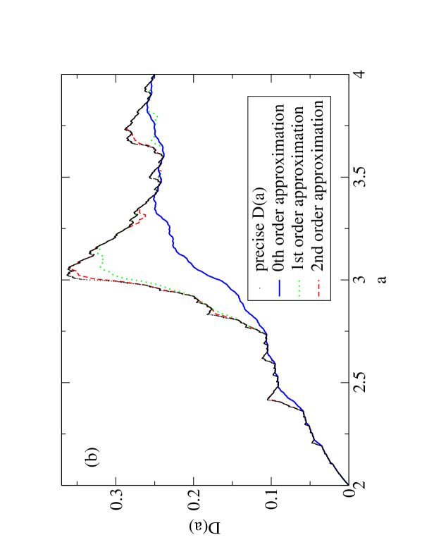
FIG. 1.: Diffusion coefficient $D(a)$ for the one-dimensional map shown in the upper left part of (a), where $a$ is the slope of the map. The dots are obtained from the method of Refs. [2–4], the different lines correspond to different levels of approximations based on the Green-Kubo formula Eq. (5). In (a) the approximations were computed from Eq. (10) assuming a constant invariant density, in (b) they are from Eq. (11) which includes the exact invariant density. Any error bars are smaller than visible. All quantities here and in the following figures are without units.

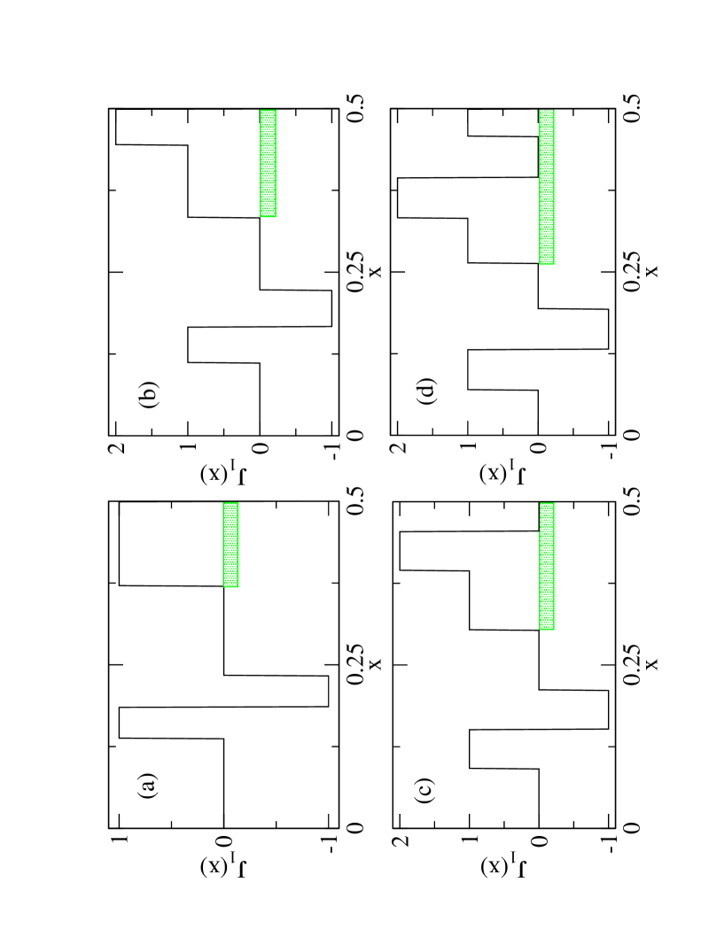
FIG. 2.: Jump velocity function $J_{1}(x)$ as defined by Eq. (14) which gives the integer value of the displacement of a particle starting at some initial position $x$. Shown are results for different values of the slope $a$. It is (a) $a=2.7$, (b) $a=3.0$, (c) $a=3.3$, (d) $a=3.8$. The shaded bar marks the subinterval where the jump velocity $j(x_{n})$ defined in Eq. (6) is equal to one.

FIG. 3.: Jump velocity function $J_{n}(x)$ as defined by Eq. (14) at the fixed parameter value $a=3.8$ for the different number of time steps (a) $n=0$, (b) $n=1$, (c) $n=2$, (d) $n=3$. Again, the shaded bar marks the subinterval where the jump velocity $j(x_{n})$ defined in Eq. (6) is equal to one.

FIG. 4.: Geometry of the periodic Lorentz gas with the gap size $w$ as control parameter. The hatched area related to (1) marks a so-called trapping region, the arrow gives the lattice vector connecting the center of this trap to the next one above. In (2) three lattice vectors are introduced and labeled with the symbols $l,r,z$. They indicate the positions where particles move along the hexagonal lattice of Wigner-Seitz cells, starting from the trap $z$, within two time steps of length $\tau$. (3) depicts the situation after three time steps $\tau$ with the different lattice vectors associated to symbol sequences of length two.

FIG. 5.: Diffusion coefficient $D(w)$ for the periodic Lorentz gas as a function of the gap size $w$ as a control parameter. The computer simulation results for $D(w)$ are from Ref. [8], error bars are much smaller than the size of the symbols. The other lines correspond to different levels of the approximation Eq. (18), the last approximation (again with symbols) is from Eq. (24).

REFERENCES

- [1] J.R. Dorfman, An Introduction to Chaos in Nonequilibrium Statistical Mechanics (Cambridge University Press, Cambridge, 1999).
- [2] P. Gaspard, Chaos, Scattering, and Statistical Mechanics (Cambridge University Press, Cambridge, 1998).
- [3] R. Klages and J.R. Dorfman, Phys. Rev. Lett. 74, 387 (1995).
- [4] R. Klages, Deterministic diffusion in one-dimensional chaotic dynamical systems (Wissenschaft & Technik-Verlag, Berlin, 1996).
- [5] R. Klages and J.R. Dorfman, Phys. Rev. E 59, 5361 (1999).
- [6] I. Dana, N. Murray, and I. Percival, Phys. Rev. Lett. 65, 1693 (1989).
- [7] A. Rechester and R. White, Phys. Rev. Lett. 44, 1586 (1980).
- [8] P. Leboeuf, Physica D 116, 2767 (1998).
- [9] R. Klages and C. Dellago, J. Stat. Phys. 101, 145 (2000).
- [10] T. Harayama and P. Gaspard, Phys. Rev. E 64, 036215 (2001).
- [11] P. Gaspard and R. Klages, Chaos 8, 409 (1998).
- [12] B. Moran and W. Hoover, J. Stat. Phys. 48, 709 (1987).
- [13] D. Weiss et al., Phys. Rev. Lett. 66, 2790 (1991).
- [14] H. Fujisaka and S. Grossmann, Z. Physik B 48, 261 (1982).
- [15] P. Gaspard, J. Stat. Phys. 68, 673 (1992).
- [16] T. Geisel and J. Nierwetberg, Phys. Rev. Lett. 48, 7 (1982).
- [17] M. Schell, S. Fraser, and R. Kapral, Phys. Rev. A 26, 504 (1982).
- [18] R. Klages and J.R. Dorfman, Phys. Rev. E 55, R1247 (1997).
- [19] B. Mandelbrot, The Fractal Geometry of Nature (W.H. Freeman and Company, San Francisco, 1982).
- [20] L. A. Bunimovich and Y. G. Sinai, Commun. Math. Phys. 78, 247 (1980).
- [21] J. Machta and R. Zwanzig, Phys. Rev. Lett. 50, 1959 (1983).
- [22] P. Gaspard, Phys. Rev. E 53, 4379 (1996).
- [23] T. Harayama (unpublished).
- [24] P. Cvitanović, J.-P. Eckmann, and P. Gaspard, Chaos, Solitons, Fractals 6, 113 (1995).
- [25] P. Cvitanovic, P. Gaspard, and T. Schreiber, Chaos 2, 85 (1992).
- [26] J.R. Dorfman and H. van Beijeren, in Statistical mechanics, edited by B. Berne (Plenum Press, New York, 1977), Vol. B, Chap. 3, pp. 65–179.
- [27] N. Korabel and R. Klages (unpublished).
- [28] T. Harayama, R. Klages, and P. Gaspard (unpublished).
- [29] A. Lasota and M. Mackey, Chaos, Fractals, and Noise, Vol. 97 of Applied mathematical sciences, 2nd ed. (Springer, Berlin, 1994).