Finite-size scaling in the steady state of the fully asymmetric exclusion process

Abstract

Finite-size scaling expressions for the current near the continuous phase transition, and for the local density near the first-order transition, are found in the steady state of the one-dimensional fully asymmetric simple-exclusion process (FASEP) with open boundaries and discrete-time dynamics. The corresponding finite-size scaling variables are identified as the ratio of the chain length to the localization length of the relevant domain wall.

I Introduction

We consider the fully asymmetric simple-exclusion process (FASEP) on a finite chain of $L$ sites with open boundaries. For mathematical definition of the exclusion processes we refer the reader to the book [1], and for a recent review on the relevant class of exactly solvable models for many-body systems far from equilibrium to [2], see also [3]. We recall that each site $i\in\{1,2,\dots,L\}$ of the chain is either empty or occupied by exactly one particle. The particles obey a discrete-time stochastic dynamics according to which they hop with probability $p$ only to empty nearest-neighbor sites to the right. The open boundary conditions imply that at each time step (update of the whole chain) a particle is injected with probability $\alpha$ at the left end of the chain ($i=1$), and removed with probability $\beta$ at the right end ($i=L$). The order in which the local hopping, injection and particle removal takes place is specified by one of the basic discrete-time updates, see [4]. Here we explicitly consider the case of forward-ordered sequential update.

We mention that the case of random-sequential update was solved first by using the recursion relations method [5], [6], and then by means of the matrix-product Ansatz (MPA) [7]. Next, the method of MPA was successfully applied for obtaining the steady-state properties in all the basic cases of true discrete-time dynamics: forward- ($\rightarrow$) and backward-ordered ($\leftarrow$) sequential [8], [9], [10], sublattice-parallel ($\mbox{s-}\parallel$) [11], [12], and, finally, fully parallel dynamics [13], [14].

The phase diagram for all the discrete-time updates has the same structure, as shown in Fig. 1: it contains a maximum-current (m.c.), low-density (l.d.), and high-density (h.d.) phases. The maximum-current phase is separated by lines of continuous phase transitions, $(\alpha=\alpha_{c},\;\beta_{c}\leq\beta\leq 1)$ and $(\beta=\beta_{c},\;\alpha_{c}\leq\alpha\leq 1)$, from the low-density and high-density phases, respectively. Here $\alpha_{c}$ and $\beta_{c}$ are the critical values of the injection and removal probabilities:

$$\alpha_{c}=\beta_{c}=1-\sqrt{1-p}.$$ (1)

The above phases were identified with respect to the analytic form of the bulk current: for fixed $p$, the current in the low- (high-) density phase depends only on $\alpha$ ($\beta$), and in the maximum-current phase it is independent of both $\alpha$ and $\beta$. On crossing the borderline between the maximum-current and the low- (high-) density phase, the current itself and its first derivative with respect to $\alpha$ ($\beta$) change continously, and the second derivative with respect to $\alpha$ ($\beta$) udergoes a finite jump. The coexistence line between the low- and high-density phases is given by $(\alpha=\beta,\;0\leq\beta\leq\beta_{c})$; on crossing it the bulk density undergoes a finite jump.

Here, the exact finite-size expressions for the current and local density in the steady state of FASEP with open boundaries and forward-ordered sequential update, derived in [10], are analysed within the framework of finite-size scaling (FSS) at continuous (for the current) and first-order (for the density) phase transitions. The appropriate scaling variables are identified and the corresponding scaling functions for the current and local desity are explicitly obtained. The notions of the Privman-Fisher anisotropic FSS have been recently extended to non-equilibrium systems belonging to the directed percolation and diffusion-annihilation universality classes, [3], [15], [16]. To the best of our knowledge, the present study is the first step in the analytic confirmation of FSS for an exactly solved model of a driven lattice gas with open boundaries. Since we are dealing with phase transitions in the steady-state of the FASEP with discrete-time updates, the equvalent two-dimensional lattice model is infinite in the temporal direction but finite in the spatial one.

Note that the current has the same value in the cases of forward-ordered ($\rightarrow$), backward-ordered ($\leftarrow$) sequential, and sublattice-parallel ($\mbox{s-}\parallel$) dynamics, i.e., $J_{L}^{\rightarrow}=J_{L}^{\leftarrow}=J_{L}^{\mbox{s-}\parallel}$. The corresponding local densities at site $i\in\{1,\dots,L\}$ are related to each other [12]:

$$\rho_{L}^{\rightarrow}(i)=\rho_{L}^{\leftarrow}(i)-J_{L}^{\rightarrow},\qquad\rho_{L}^{\mbox{s-}\parallel}(i)=\left\{\begin{array}[]{ll}\rho_{L}^{\rightarrow}(i),&\quad\mbox{$i$ odd}\\ \rho_{L}^{\leftarrow}(i),&\quad\mbox{$i$ even}.\end{array}\right.$$ (2)

As shown in [13], the current $J_{L}^{\parallel}$ and local density $\rho_{L}^{\parallel}(i)$ for the FASEP with fully parallel update can be simply expressed in terms of those for the forward-ordered sequential update:

$$J_{L}^{\parallel}={J_{L}^{\rightarrow}\over 1+J_{L}^{\rightarrow}},\qquad\rho_{L}^{\parallel}(i)={\rho_{L}^{\rightarrow}(i)+J_{L}^{\rightarrow}\over 1+J_{L}^{\rightarrow}}.$$ (3)

Due to these relations, the results derived here suffice to explicitly obtain the current and density FSS functions for each of the basic discrete-time updates.

Concerning the notation, we note that the exact finite-chain results obtained in [10] are conveniently expressed in terms of the parametrs

$$d=\sqrt{1-p},\quad a=d+d^{-1},\quad\xi={p-\alpha\over\alpha d},\quad\eta={p-\beta\over\beta d},$$ (4)

which will be used here too.

II Finite-size scaling at the continuous phase transition

Let us consider first the continuous phase transition across the boundary $\alpha=\alpha_{c},\;\beta_{c}\leq\beta\leq 1$ between the low-density phase and the maximum-current phase. In terms of the variables (4) the equation of this boundary reads $\xi=1,\;-d\leq\eta\leq 1$; the m.c. phase occupies the region $-d\leq\xi\leq 1,\;-d\leq\eta\leq 1$, and the region $\xi>1\geq\eta\geq-d$, called region AII, lies in the l.d. phase, see Fig. 1.

According to the basic FSS hypotheses, the FSS variable in the case of a continuous transition, characterized by diverging bulk correlation length $\lambda$, should be given by the ratio $L/\lambda$, where $L$ is the finite-size of the system. As it is well known, in the case at hand the inverse correlation length $\lambda_{\xi}^{-1}$ in the l.d. phase is, see, e.g., [14], [17],

$$\lambda_{\xi}^{-1}=\ln\left[1+{(\xi-1)^{2}\over\xi(a+2)}\right],\quad(\xi\geq 1),$$ (5)

and $\lambda_{\xi}^{-1}\equiv 0$ in the m.c. phase. Hence, the FSS variable as $L\rightarrow\infty$ and $\xi\rightarrow 1^{+}$ is expected to be given by

$$L/\lambda_{\xi}\simeq{L(\xi-1)^{2}\over\xi(a+2)}:=x_{1}^{2}(L,t),$$ (6)

where

$$x_{1}(L,t)\simeq C_{1}tL^{1/2},\quad C_{1}=(a+2)^{-1/2},\quad t=\xi-1.$$ (7)

We emphasize that here we study a boundary induced non-equilibrium phase transition, and the physical quantity which measures the distance from the steady-state critical point is related to the injection probability: $t=\xi-1\sim 1-\alpha/\alpha_{c}$.

Consider now the finite-size current $J_{L}(\xi,\eta)=Z_{L-1}(\xi,\eta)/Z_{L}(\xi,\eta)$, where $Z_{L}(\xi,\eta)$ is the normalization constant of the steady-state probability for a lattice of $L$ sites. The following exact representation of $Z_{L}(\xi,\eta)$ in the subregion AII of the low-density phase ($\xi>1\geq\eta$) has been found in [10]:

$$Z_{L}^{\rm AII}(\xi,\eta)=\left({d\over p}\right)^{L}{\xi-\xi^{-1}\over\xi-\eta}(a+\xi+\xi^{-1})^{L}+Z_{L}^{\rm m.c.}(\xi,\eta).$$ (8)

Here the expression for the normalization constant in the maximum-current phase ($\xi\not=\eta$),

$$Z_{L}^{\rm m.c.}(\xi,\eta)=\left({d\over p}\right)^{L}\left[{\xi\over\xi-\eta}I_{L}(\xi)+{\eta\over\eta-\xi}I_{L}(\eta)\right],$$ (9)

involves the integral

$$I_{L}(\xi)=\frac{2}{\pi}\int_{0}^{\pi}{\rm d}\phi{(a+2\cos\phi)^{L}\sin^{2}\phi\over 1-2\xi\cos\phi+\xi^{2}},$$ (10)

which is a non-analytic function of $\xi$ at $\xi=1$. For all finite $L$ the normalization constant $Z_{L}^{\rm AII}(\xi,\eta)$ in region AII represents an analytic continuation of $Z_{L}^{\rm m.c.}(\xi,\eta)$ from the domain $|\xi|<1$ to the domain $|\xi|>1$, see [10].

A direct application of Laplace’s method for evaluation of the integral (10) as $L\rightarrow\infty$ shows that it changes its leading-order asymptotic behavior from $O(L^{-3/2})$ for $\xi\not=1$ to $O(L^{-1/2})$ for $\xi=1$, see Eq. (14) in [17]. The finite-size expression that interpolates between these limiting asymptotic forms can be readily obtained by using small-argument expansion of the trigonometric functions in the integrand. The result for $x_{1}(L,t)=O(1)$ is

$$I_{L}(\xi)\simeq{(a+2)^{L+1/2}\over\xi\sqrt{\pi L}}X(|x_{1}|),$$ (11)

where the FSS function $X(\cdot)$ is given by

$$X(x)=1-\sqrt{\pi}x{\rm e}^{x^{2}}[1-\Phi(x)],\quad\Phi(x)={2\over\sqrt{\pi}}\int_{0}^{x}{\rm e}^{-t^{2}}{\rm d}t.$$ (12)

Thus, keeping the $1/L$ corrections to the finite-size scaling form, we obtain

$$Z_{L}^{\rm m.c.}(\xi,\eta)\simeq\left({d\over p}\right)^{L}{1\over\xi-\eta}{(a+2)^{L+1/2}\over\sqrt{\pi L}}\left[X(|x_{1}|)-{\eta\over(1-\eta)^{2}}{a+2\over 2L}\right].$$ (13)

The small- and large-argument asymptotic behavior of $X(\cdot)$ readily follows from that of the Fresnel integral $\Phi(\cdot)$:

$$X(x)=\left\{\begin{array}[]{ll}1-\sqrt{\pi}x+O(x^{2}),&\mbox{\rm as}\quad x\rightarrow 0,\\ {1\over 2}x^{-2}-{3\over 4}x^{-4}+O(x^{-6}),&\mbox{\rm as}\quad x\rightarrow\infty.\end{array}\right.$$ (14)

Let us first evaluate the asymptotic behvior of the finite-size correction to the bulk current in the maximum-current phase,

$$J_{L}^{\rm m.c.}(\xi,\eta)-J_{\infty}^{\rm m.c.}={Z_{L-1}^{\rm m.c.}(\xi,\eta)\over Z_{L}^{\rm m.c.}(\xi,\eta)}-{p\over d(a+2)},$$ (15)

as $L\rightarrow\infty$ and $\xi\rightarrow 1^{-}$ at fixed $\eta<1$. We readily obtain in the leading order of magnitude,

$$\xi[(a+2)I_{L-1}(\xi)-I_{L}(\xi)] \simeq {|1-\xi|^{3/2}\over\xi^{3/2}}{2\over\pi}\int_{0}^{\infty}{\rm d}x{{\rm e}^{-x_{1}^{2}x^{2}}x^{4}\over 1+x^{2}}$$ (16)

$$= {(a+2)^{3/2}\over 2\sqrt{\pi}L^{3/2}}[1-2x_{1}^{2}X(|x_{1}|)].$$ (17)

Hence we derive

$$J_{L}^{\rm m.c.}(\xi,\eta)-J_{\infty}^{\rm m.c.}\simeq{1\over L}{p\over 2d(a+2)}\left[{1-2x_{1}^{2}X(|x_{1}|)\over X(|x_{1}|)}\right].$$ (18)

The asymptotic behavior of the above finite-size correction to the current as $x_{1}\rightarrow 0^{-}$ (say, as $\xi\rightarrow 1^{-}$ at large fixed $L$) follows from Eq. (14):

$$J_{L}^{\rm m.c.}(1,\eta)-J_{\infty}^{\rm m.c.}\simeq{1\over L}{p\over 2d(a+2)}.$$ (19)

In the limiting case $x_{1}\rightarrow-\infty$ (say, $L\rightarrow\infty$ at $\xi<1$ fixed close to unity), we obtain that the finite-size correction is again of the order $O(L^{-1})$:

$$J_{L}^{\rm m.c.}(\xi,\eta)-J_{\infty}^{\rm m.c.}\simeq{1\over L}{3p\over 2d(a+2)}.$$ (20)

Consider next the asymptotic behvior of the finite-size correction to the bulk current in the low-density phase,

$$J_{L}^{\rm AII}(\xi,\eta)-J_{\infty}^{\rm l.d.}(\xi)={Z_{L-1}^{\rm AII}(\xi,\eta)\over Z_{L}^{\rm AII}(\xi,\eta)}-{p\over d(a+\xi+\xi^{-1})},$$ (21)

as $L\rightarrow\infty$ and $\xi\rightarrow 1^{+}$ at fixed $\eta<1$. With the aid of the identities:

$$\xi[(a+\xi+\xi^{-1})I_{L-1}(\xi)-I_{L}(\xi)]=I_{L-1}(0),$$ (22)

$$\eta[(a+\xi+\xi^{-1})I_{L-1}(\eta)-I_{L}(\eta)]=I_{L-1}(0)+(\xi-\eta)(\eta-\xi^{-1})I_{L-1}(\eta),$$ (23)

we obtain in the leading order:

$$J_{L}^{\rm AII}(\xi,\eta)-J_{\infty}^{\rm l.d.}(\xi)\simeq{1\over L}{p\over 2d(a+2)}\left[{1\over 2\sqrt{\pi}x_{1}{\rm e}^{x_{1}^{2}}+X(x_{1})}\right].$$ (24)

Hence, by using Eq. (14) we readily derive the asymptotic behavior of the above finite-size correction as $x_{1}\rightarrow 0^{+}$ (say, as $\xi\rightarrow 1^{+}$ at large fixed $L$):

$$J_{L}^{\rm AII}(1,\eta)-J_{\infty}^{\rm l.d.}(1)\simeq{1\over L}{p\over 2d(a+2)}.$$ (25)

In the other limiting case $x_{1}\rightarrow\infty$ (say, $L\rightarrow\infty$ at $\xi>1$ fixed close to unity), we obtain that the finite-size corrections to the current are exponentially small:

$$J_{L}^{\rm AII}(\xi,\eta)-J_{\infty}^{\rm l.d.}(\xi)=O\left(x_{1}^{-1}{\rm e}^{-x_{1}^{2}}\right).$$ (26)

As a finite-size order parameter of the continuous phase transition one could consider the difference in the finite-size currents:

$$\Delta_{L}(\xi,\eta):=J_{L}^{\rm m.c.}(\xi,\eta)-J_{L}^{\rm AII}(\xi,\eta)\quad(\xi>1,\eta<1).$$ (27)

Here $J_{L}^{\rm m.c.}(\xi,\eta)$ represents the analytic expression for the finite-size current in the maximum-current phase, i.e., $J_{L}^{\rm m.c.}=Z_{L-1}^{\rm m.c.}/Z_{L}^{\rm m.c.}$ with $Z_{L}^{\rm m.c.}$ defined by Eqs. (9) and (10), evaluated in subregion AII of the low-density phase (at $\xi>1,\eta<1$). For the corresponding bulk quantity we have

$$\Delta_{\infty}(\xi)=J_{\infty}^{\rm m.c.}-J_{\infty}^{\rm l.d.}(\xi)={(\alpha-\alpha_{c})^{2}\over p(1-\alpha)},$$ (28)

which suggests the critical exponent for the order parameter $\beta=2$. In the finite-size case, by taking into account that

$${p\over d(a+2)}-{p\over d(a+\xi+\xi^{-1})}={1\over L}{p\over d(a+2)}{x_{1}^{2}\over 1+x_{1}^{2}/L},$$ (29)

and combining the above results, we obtain in the leading order

$$\Delta_{L}(\xi,\eta)\simeq{1\over L}{p\over 2d(a+2)}\left\{{x_{1}\over X(x_{1})\left[x_{1}+{1\over 2\sqrt{\pi}}{\rm e}^{-x_{1}^{2}}X(x_{1})\right]}\right\}.$$ (30)

Since the high-density phase maps onto the low-density phase under the exchange of arguments $\xi\leftrightarrow\eta$ (equivalently, $\alpha\leftrightarrow\beta$), the FSS properties of the continuous transition across the boundary $\beta=\beta_{c},\;\alpha_{c}\leq\alpha\leq 1$ between the high-density phase and the maximum-current phase follow trivially from the above results and the particle-hole symmetry.

III Finite-size scaling at the first-order transition

In the thermodynamic limit the first-order phase transition, which occurs across the borderline $\beta=\alpha,\;0\leq\alpha\leq\alpha_{c}$ ($\eta=\xi,\;\xi\geq 1$) between subregions AI and BI, manifests itself by a finite jump in the bulk density:

$$\left.\rho_{\rm bulk}^{\rm h.d.}(\eta)-\rho_{\rm bulk}^{\rm l.d.}(\xi)\right|_{\xi=\eta}={\eta-\eta^{-1}\over a+\eta+\eta^{-1}}>0.$$ (31)

Quite peculiarly, this transition is characterised by another diverging correlation length

$$\lambda^{-1}=|\lambda_{\xi}^{-1}-\lambda_{\eta}^{-1}|={1-\eta^{-2}\over a+\eta+\eta^{-1}}|\xi-\eta|+O(|\xi-\eta|^{2}),$$ (32)

which suggests the finite-size scaling variable

$$\tilde{x_{2}}:=L/\lambda\simeq C_{2}|h|L,\quad C_{2}={1-\eta^{-2}\over a+\eta+\eta^{-1}},\quad h=\xi-\eta.$$ (33)

Our analysis starts with the exact result found for the finite-chain local density $\rho_{L}^{\rm D}(i;\xi,\eta)$ in region D$=$AI$\cup$BI of the phase diagram, see Eqs. (4.21) and (A13) in [10]. This result can be cast in the form ($\xi\not=\eta$):

$$\rho_{L}^{\rm D}(i;\xi,\eta)={1-p\over p}J_{L}^{\rm D}(\xi,\eta)+\widetilde{\Omega}_{L}^{\rm D}(i;\xi,\eta),$$ (34)

where,

$$\widetilde{\Omega}_{L}^{\rm D}(i;\xi,\eta)=\left(\frac{d}{p}\right)^{L}{(a+2)^{L-1}\over(\xi-\eta)Z_{L}^{\rm D}}\left[(1-\xi^{-2}){\rm e}^{(L-1)/\lambda_{\xi}}\right.$$ (35)

$$\left.+(\xi-\xi^{-1})(\eta-\eta^{-1}){\rm e}^{(i-1)/\lambda_{\xi}}{\rm e}^{(L-i)/\lambda_{\eta}}-(\eta^{2}-1){\rm e}^{(L-1)/\lambda_{\eta}}\right]$$ (36)

$$-\left(\frac{d}{p}\right)^{L}{(a+2)^{L-1}\over Z_{L}^{\rm D}}\left[(\xi-\xi^{-1}){\rm e}^{(i-1)/\lambda_{\xi}}\left({p\over d}\right)^{L-i}{Z_{L-i}^{\rm m.c.}\over(a+2)^{L-i}}\right.$$ (37)

$$\left.-(\eta-\eta^{-1}){\rm e}^{(L-i)/\lambda_{\eta}}\left({p\over d}\right)^{i-1}{Z_{i-1}^{\rm m.c.}\over(a+2)^{i-1}}\right]$$ (38)

$$+\frac{d}{2p}{1\over Z_{L}^{\rm D}}\left[F_{L}(i;\xi,\eta)-(\xi-\eta)Z_{i-1}^{\rm m.c.}Z_{L-i}^{\rm m.c.}+\frac{p}{d}Z_{L}^{\rm m.c.}-aZ_{L-1}^{\rm m.c.}\right].$$ (39)

For brevity of notation we have omitted the arguments $\xi$ and $\eta$ of the function $Z_{L}(\xi,\eta)$. Here the term $F_{L}(i)=F_{L}(i;\xi,\eta)$ is the antisymmetric (with respect to the center of the chain) function of the integer coordinate $i$, $F_{L}(i;\xi,\eta)=-F_{L}(L-i+1;\xi,\eta)$, defined for $1\leq i\leq[L/2]$ (where $[x]$ denotes the integer part of $x$) by the equation

$$F_{L}(i;\xi,\eta)=\left({d\over p}\right)^{L-1}(1-\xi\eta)\sum_{n=0}^{L-2i}I_{L-i-n-1}(\xi)I_{i+n-1}(\eta).$$ (40)

The normalization constant in the region D$=$AI$\cup$BI ($\xi>1,\eta>1$) for $\xi\not=\eta$ is given by

$$Z_{L}^{\rm D}(\xi,\eta)=\left({d\over p}\right)^{L}{(a+2)^{L}\over\xi-\eta}\left[(\xi-\xi^{-1}){\rm e}^{L/\lambda_{\xi}}-(\eta-\eta^{-1}){\rm e}^{L/\lambda_{\eta}}\right]+Z_{L}^{\rm m.c.}(\xi,\eta).$$ (41)

Let us analyse this expression when $\xi=\eta+h$, $h\rightarrow 0$. For $Z_{L}^{\rm m.c.}(\eta+h,\eta)$ we have

$$Z_{L}^{\rm m.c.}(\eta+h,\eta) = \left({d\over p}\right)^{L}{1\over h}[(\eta+h)I_{L}(\eta+h)-\eta I_{L}(\eta)]$$ (42)

$$= -\left({d\over p}\right)^{L}(\eta^{2}-1)K_{L}(\eta)+O(h),$$ (43)

where

$$K_{L}(\eta)=\frac{2}{\pi}\int\limits_{0}^{\pi}{\rm d}\phi{(a+2\cos\phi)^{L}\sin^{2}\phi\over(1-2\eta\cos\phi+\eta^{2})^{2}}.$$ (44)

For $\xi=\eta+h$, as $L\rightarrow\infty$ and $h\rightarrow 0$ we have

$$L/\lambda_{\eta+h}=L/\lambda_{\eta}+C_{2}hL+O(Lh^{2}),$$ (45)

hence

$$Z_{L}^{\rm D}(\eta+h,\eta)=\left({d\over p}\right)^{L}(a+2)^{L}\left[(\eta-\eta^{-1}){\rm e}^{L/\lambda_{\eta}}{{\rm e}^{C_{2}hL}-1\over h}+O(1)\right].$$ (46)

Next, by using the upper bound $I_{k}(\xi)\leq(a+2)^{k}I_{0}(\xi)$, where $I_{0}(\xi)=1$ for $|\xi|\leq 1$ and $I_{0}(\xi)=\xi^{-2}$ for $|\xi|\geq 1$, one easily obtains that in region D

$$\left|F_{L}(i;\xi,\eta)\right|\leq=\left({d\over p}\right)^{L-1}{\xi\eta-1\over\xi^{2}\eta^{2}}(L-1)(a+2)^{L-2}.$$ (47)

Therefore, in view of Eq. (46), the contribution of the term proportional to $F_{L}(i;\xi,\eta)$ into the local density is exponentially small. Thus, only the first three terms in the right-hand side of Eq. (39) contribute into the leading-order expression for $\widetilde{\Omega}_{L}^{\rm D}(\eta+h,\eta)$:

$$\widetilde{\Omega}_{L}^{\rm D}(i;\eta+h,\eta)\simeq{\eta^{-1}\over a+\eta+\eta^{-1}}+(\eta-\eta^{-1}){{\rm e}^{C_{2}hi}-1\over{\rm e}^{C_{2}hL}-1}.$$ (48)

In deriving the above expression we have assumed that both $i\gg 1$ and $L-i\gg 1$. Finally, by taking into account that

$$J_{L}^{\rm D}(\eta+h,\eta)={p\over d(a+\eta+\eta^{-1})}+O(h),$$ (49)

we obtain the leading order expression for the local density on the macroscopic scale $i/L=r$, $0<r<1$:

$$\rho_{L}^{\rm D}(rL;\xi,\eta)={1\over a+\eta+\eta^{-1}}\left[d+\eta^{-1}+(\eta-\eta^{-1}){{\rm e}^{x_{2}r}-1\over{\rm e}^{x_{2}}-1}\right].$$ (50)

Here we have introduced the FSS variable $x_{2}=C_{2}hL$, compare with Eq. (33). In the limit $x_{2}\rightarrow 0$ the above expression reduces to the well-known linear density profile on the coexistence line $\xi=\eta$:

$$\rho_{L}^{\rm D}(rL;\eta,\eta)={d+\eta^{-1}+(\eta-\eta^{-1})r\over a+\eta+\eta^{-1}}.$$ (51)

In the limit $x_{2}\rightarrow+\infty$ ($x_{2}\rightarrow-\infty$) one recovers the bulk density in the low-density (high-density) phase.

IV Discussion

The mathematical mechanism of the phase transitions in the FASEP with open boundaries has been revealed in [10] as qualitative changes in the spectrum of the lattice translation operator $C$ [18]. In the region $\xi\leq 1$, $\eta\leq 1$, occupied by the maximum-current phase, the spectrum is continuous and fills with uniform density the interval from $(d/p)(a-2)$ to $(d/p)(a+2)$. When $\eta\leq 1$ but $\xi$ becomes larger than unity, an eigenvalue

$$\nu(\xi)=(d/p)(a+\xi+\xi^{-1})$$ (52)

splits up from the continuous spectrum and dominates the properties of the low-density phase in region AII. Due to particle-hole symmetry, when $\xi\leq 1$ but $\eta$ exceeds unity, the eigenvalue that splits up from the continuous spectrum and dominates the properties of the high-density phase in region BII is $\nu(\eta)$. Thus, the logarithm of the ratio of the corresponding eigenvalue to the ceiling of the continuous spectrum defines the relevant inverse correlation length $\lambda_{\xi}^{-1}$ or $\lambda_{\eta}^{-1}$, see Eq. (5). When both $\xi>1$ and $\eta>1$, which is the case in region D$=$AI$\cup$BI, there are two eigenvalues, $\nu(\xi)$ and $\nu(\eta)$, above the continuous spectrum. Obviously, these eigenvalues become degenerate on the coexistence line $\xi=\eta>1$, which explains the appearance of the diverging correlation length (32). Note that the explicit expressions for the correlation lengths depends on the type of update only: they are the same for all the true discrete-time updates, and for the random sequential update, see Eq. (78) in [7],

$$\lambda_{\alpha}^{-1}=\ln\left[1+{(1/2-\alpha)^{2}\over\alpha(1-\alpha)}\right].$$ (53)

The physical meaning of the above correlation lengths emerges in the domain wall picture developed in [19]: the lengths $\lambda_{\xi}$, $\lambda_{\eta}$, and $\lambda$ are interpreted as localization lengths of the domain walls between the low-density/maximum-current, high-density/maximum-current, and low-density/high-density phases, respectively. The complete delocalization of the low-density/high-density domain wall on the coexistence line explains the linear density profile (51): it is the result of ensemble averaging over configurations with uniform probability distribution of the domain wall position [6].

Thus, the FSS variable for any of the phase transitions in the FASEP with open boundaries has the physical meaning of a ratio of the chain length to the localization length of the relevant domain wall. The explicit expressions for the FSS functions have been derived here for the model with forward-ordered sequential update. The corresponding expressions for the other basic discrete-time updates follow under the mappings mentioned in the Introduction.

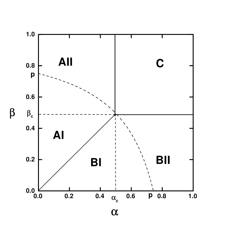
FIG. 1.: The phase diagram in the plane of the injection and removal probabilities $\alpha$ and $\beta$ (see the text) for hopping probability $p$=0.75. The maximum-current phase occupies region C. Region A$=$AI$\cup$AII corresponds to the low-density phase, and region B$=$BI$\cup$BII to the high-density phase. Subregions AI (BI) and AII (BII) are distinguished by the different analytic form of the density profile. The boundary between them, $\beta=\beta_{c}$, $0\leq\alpha\leq\alpha_{c}$ ($\alpha=\alpha_{c}$, $0\leq\beta\leq\beta_{c}$), is shown by dashed segment of a straight line. The solid line $\alpha=\beta$ between subregions AI and BI is the coexistence line of the low- and high-density phases. The curved dashed line is the mean-field line $(1-\alpha)(1-\beta)=1-p$.

REFERENCES

• [1] T. M. Liggett, Stochastic Interacting Systems: Contact, Voter and Exclusion Processes (Springer, Berlin, 1999).
• [2] G. M. SchΓΌtz, in: Phase Transitions and Critical Phenomena, Vol. 19, edited by C. Domb and J. L. Lebowitz (Academic Press, London, 2001).
• [3] H. Hinrichsen, Non-equilibrium critical phenomena and phase transitions into absorbing states, Adv. Phys. 49, 815-958 (2000).
• [4] N. Rajewsky, L. Santen, A. Schadschneider, and M. Schreckenberg, J. Stat. Phys. 92, 151 (1998).
• [5] D. Derrida, E. Domany, and D. Mukamel, J. Stat. Phys. 69, 667 (1992).
• [6] G. SchΓΌtz and E. Domany, J. Stat. Phys. 72, 277 (1993).
• [7] B. Derrida, M. R. Evans, V. Hakim, and V. Pasquier, J. Phys. A 26, 1493 (1993).
• [8] N. Rajewsky, A. Schadschneider, and M. Schreckenberg, J. Phys. A 29, L305 (1996).
• [9] A. Honecker and I. Peschel, J. Stat. Phys. 88, 319 (1997).
• [10] J. Brankov, N. Pesheva, and N. Valkov, Phys. Rev. E 61, 2300 (2000).
• [11] H. Hinrichsen, J. Phys. A 29, 3659 (1996).
• [12] N. Rajewsky and M. Schreckenberg, Physica A 245, 139 (1997).
• [13] M. R. Evans, N. Rajewsky, and E. R. Speer, J. Stat. Phys. 95, 45 (1999).
• [14] J. de Gier and B. Nienhuis, Phys. Rev. E 59, 4899 (1999).
• [15] M. Henkel and U. SchollwΓΆck, J. Phys. A 34, 3333 (2001).
• [16] M. Henkel and H. Hinrichsen, J. Phys. A 34, 1561 (2001).
• [17] J. Brankov and N. Pesheva, Phys. Rev. E 63, paper No. 046111 (2001).
• [18] R. B. Stinchcombe and G. M. SchΓΌtz, Phys. Rev. Lett. 75, 140 (1995).
• [19] A. B. Kolomeisky, G. M. SchΓΌtz, E. B. Kolomeisky, and J. P. Straley, J. Phys. A 31, 6911 (1998).
Refer to caption