Isolated resonances in conductance fluctuations and hierarchical states

Abstract

We study the isolated resonances occurring in conductance fluctuations of quantum systems with a classically mixed phase space. We demonstrate that the isolated resonances and their scattering states can be associated to eigenstates of the closed system. They can all be categorized as hierarchical or regular, depending on where the corresponding eigenstates live in the classical phase space.

]

I Introduction

The classical dynamics of a scattering system is reflected in the transport properties of its quantum mechanical analog. A prominent example in quantum chaos are the universal conductance fluctuations exhibited by a scattering system with classically completely chaotic dynamics [1]. Generic systems, however, are neither completely chaotic nor integrable, but show chaotic as well as regular motion [2]. The chaotic dynamics is strongly influenced by the presence of islands of regular motion, in particular, one finds a trapping of chaotic trajectories close to regular regions with trapping times distributed according to power laws [3]. The semiclassical analysis revealed that conductance fluctuations of generic scattering systems have corresponding power-law correlations [4, 5] and most interestingly that the graph conductance vs. control parameter is a fractal [5]. Fractal conductance fluctuations have indeed been observed experimentally in semiconductor nanostructures [6, 7] as well as numerically [8].

Surprisingly, for the cosine billiard[9, 10], a system with a mixed phase space and power-law distributed classical trapping times, a recent numerical study did not show fractal conductance fluctuations [11]. Instead, sharp isolated resonances were found with a width distribution covering several orders of magnitude. Only about one third of them can be related to quantum tunneling into the islands of regular motion [12], while the rest remained unexplained. It was later shown that conductance fluctuations for mixed systems should in general show fractal fluctuations on large scales and isolated resonances on smaller scales [13]. The isolated resonances in the scattering system were conjectured to be related to a subset of eigenstates of the closed system, namely hierarchical states [14] living in the chaotic component close to the regular regions and regular states living within the islands of regular motion [12]. This type of behavior was obtained for a quantum graph which modeled relevant features of a mixed phase space [13].

The purpose of the present paper is to establish the origin of all isolated resonances for a system with a mixed phase space. To this end, we study the cosine billiard for suitable parameters in a three-fold way: (i) as a quantum scattering system, (ii) as a closed quantum system, and (iii) its classical phase-space structures. We find that the resonances have scattering states and corresponding eigenstates of the closed system that live in the hierarchical and regular part of phase space. The number of resonances of each type is directly related to the corresponding volumes in the classical phase space. Each resonance width is quite well described by the strength of the corresponding eigenfunction at the billiard boundary. Exceptions are shown to arise from the presence of avoided crossings in the closed system. It is demonstrated that the simultaneous appearance of fractal conductance fluctuations and isolated resonances, as observed in a quantum graph model [13], would for our system with a mixed phase space require much higher energies. These are currently computationally inaccessible.

In the following section, we define the model we use to study the relation between the scattering resonances and the eigenstates of the corresponding closed system. Our main results on the classification of resonant scattering states and corresponding eigenstates of the closed system into hierarchical and regular are presented in Secs. III and IV. The role of partial transport barriers is analyzed in Sec. V. In Sec. VI we discuss the effect of avoided crossings on the assignment of resonances of the open billiard to eigenstates of the closed system and Sec. VII gives a summary of the results. Finally, the Appendix contains some details of the numerical methods employed in the present work.

II The Model

We study the cosine billiard [9, 10], either closed or with semi-infinite leads attached. The boundaries of the billiard are hard walls (i.e. Dirichlet boundary conditions) at $y=0$ and

$$y(x)=W+\frac{M}{2}\left(1-\cos\left(\frac{2\pi x}{L}\right)\right),$$ (1)

for $0\leq x\leq L$ (see Fig. 1a). In the open billiard two semi-infinite leads of width $W$ are attached at the openings at $x=0$ and $x=L$, while in the closed billiard the openings are closed by hard walls. The classical phase-space structure can be changed by varying the ratios $W/L$ and $M/L$. For $M/L=0$ the dynamics is integrable and for example for $M/L=1/2$ and $W/L=1$ the dynamics appears to be ergodic (at least the islands of regular motion, if any, are very small) [9].

In the present work, we use the same parameters as in Ref. [11], namely $W/L=0.18$ and $M/L=0.11$, for which the I- and M-shaped orbits depicted in Fig. 1a are stable. The corresponding Poincaré section is shown in Fig. 1b. We use Poincaré-Birkhoff coordinates $(s,p)$, where $s$ is the arclength along the upper boundary of the billiard with length $L^{\prime}\approx 1.029\,L$ and $p$ is the projection of the unit momentum vector after the reflection on the tangent in the point $s$.

Quantum mechanically, for a given wave number $k_{F}$ the number $N$ of transmitting modes in a lead of width $W$ is the largest integer with $N\leq k_{F}W/\pi$. We measure energies in units of the energy $E_{0}=\hbar^{2}\pi^{2}/(2mW^{2})$ of the lowest mode in such a lead, i.e., $E=\hbar^{2}k_{F}^{2}/(2mE_{0})=(k_{F}W/\pi)^{2}\geq N^{2}$. The larger the number $N$ of modes is, the more details of the classical phase space can be resolved by quantum mechanics. At the same time the computational effort increases with $N^{4}$ and we compromise, as in Ref. [11], on the case of $N=45$ transmitting modes in the energy range $E\in[2026,2100]$.

FIG. 1.: (a) The cosine billiard with semi-infinite leads (short dashed lines) and hard walls for closing the system (dotted lines) for $W/L=0.18$ and $M/L=0.11$. Also shown are the two most prominent stable periodic orbits for these parameters (long dashed lines). (b) Poincaré section of some regular and one chaotic orbit for the above parameters in Poincaré-Birkhoff coordinates $p$ vs arclength $s$ along the upper boundary of the billiard. A major island at $(s,p)=(L^{\prime}/2,0)$ around the elliptic I-shaped orbit and 4 smaller islands surrounding the M-shaped orbit can be seen.

III Resonances and scattering states

Resonances in the scattering system, which have been observed as isolated features in conductance fluctuations [11], were identified by isolated peaks in the Wigner-Smith time delay $\tau$ of the system. The time delay is given by

$$\tau=\frac{-i\hbar}{2N}\mbox{Tr}\,(S^{\dagger}dS/dE),$$ (2)

where $2N$ is the dimension of the $S$-matrix. The calculation of $S$ and $\tau$ was already outlined in Ref. [11] and is presented in greater detail in Appendix A.

FIG. 2.: Wigner-Smith delay time $\tau$ vs energy $E$. For each resonance a corresponding eigenstate of the closed system was found and the labels indicate whether it lives in the regular ($r$) or hierarchical ($h$) region of phase space.

In Fig. 2 we show the Wigner-Smith time delay $\tau$ [in units of $\hbar/E_{0}=2mW^{2}/(\hbar\pi^{2})$] for $E\in[2026,2100]$. The isolated resonances found in Ref. [11] are clearly seen. Each isolated resonance $E_{{\rm res},i}$ has a Breit-Wigner shape

$$\tau_{i}(E)=\tau_{i}\,\frac{\Gamma_{i}^{2}/4}{(E-E_{{\rm res},i})^{2}+\Gamma_{i}^{2}/4},$$ (3)

with $\tau_{i}\Gamma_{i}=2/N$. Note that the heights $\tau_{i}$ and the corresponding widths $\Gamma_{i}$ of the individual resonances cover several orders of magnitude.

In order to elucidate the nature of the resonances, we calculated the scattering states inside the open billiard. For a given configuration of waves incoming in both leads, the knowledge of the $S$-matrix allows the determination of the outgoing waves and hence the wavefunction amplitudes at the openings of the billiard. Since the $S$-matrix is defined between asymptotic, propagating modes, this procedure neglects the contribution of evanescent modes in the leads in the vicinity of the billiard. The wavefunction amplitudes at the openings can then be used as boundary conditions for the solution of the Schrödinger equation inside the billiard. For the examples of scattering states presented below, we occupied the 10 topmost modes incoming from the left with equal amplitudes. Similar pictures were obtained for other boundary conditions.

For the comparison of the scattering states with the classical phase-space structures we have calculated Husimi projections $H^{sc}(s,p)$. Similar to the case of closed billiards, see sec. IV, we define these by the projection of the scattering state onto a coherent state on the upper boundary of the billiard,

$$H^{sc}(s,p) = |\langle\partial_{{\bf n}}\psi|\phi^{\text{coherent}}_{\gamma}(s,p)\rangle|^{2}$$ (4)

$$= \left|\int^{L^{\prime}}_{0}ds^{\prime}\partial_{{\bf n}}\psi^{*}(s^{\prime})e^{ikp(s^{\prime}-s)-\frac{1}{2}k(s^{\prime}-s)^{2}}\right|^{2},$$ (5)

with $k=\sqrt{E}\pi/W$. Here $\partial_{{\bf n}}\psi(s)={\bf n}(s)\cdot{\bf\nabla}\psi({\bf q}(s))$ is the normal derivative of the scattering state on the upper boundary. ${\bf n}(s)$ is the normal vector and ${\bf q}(s)$ is the position of the boundary as a function of arc length $s$. Note that these Husimi projections are not normalized and are influenced by the openings over a range of a few Fermi wavelengths. Also they do not include the full billiard boundary and therefore no periodization of the coherent state has been used.

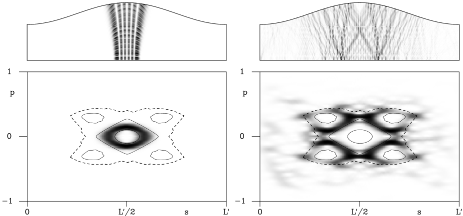
FIG. 3.: Resonant scattering states (top row) and Husimi projections (bottom row) onto the classical Poincaré section with KAM-tori (solid lines) and a partial transport barrier (dashed line). Two example at resonance energies 2029.172 (left) and 2041.109 (right) are shown. They live in the regular and the hierarchical region of phase space, respectively. For the representation of the scattering states a superposition with equal weight of the 10 topmost modes incoming from the left is shown.

As a first example, we present in Fig. 3 on the left the scattering state at an energy of approximately 2029.172, the center energy of the sharpest observed resonance. Obviously, the scattering state is associated with the I-shaped periodic orbit. The wavefunction amplitude is concentrated near the orbit and the Husimi projection lives predominantly inside the central stable island of the classical phase space. For comparison, we present in Fig. 3 on the right the scattering state at energy 2041.109. The width of the resonance at this energy is about $6\cdot 10^{7}$ times larger than the width of the sharpest resonance. Evidently, this resonance is not related to the stable islands in phase space. In contrast, by comparing with the superimposed KAM-tori of the Poincaré section and a partial transport barrier surrounding the island hierarchy (see Section V), we see that the Husimi projection lives in the hierarchical region between the islands and a partial transport barrier.

As scattering states allow a great variability in the boundary conditions, e.g., the incoming modes, we do not use them for a detailed analysis of the isolated resonances. Instead we consider the corresponding eigenstates of the closed system in the next section.

IV Resonances and corresponding eigenstates

In this section we want to demonstrate that the isolated resonances of the conductance fluctuations and their scattering states have corresponding eigenstates of the closed billiard. In particular, we will show that all these eigenstates live in the hierarchical and regular part of phase space, as was conjectured in Ref. [13]. This allows a labeling of all isolated resonances appearing in Fig. 2.

For the closed system the eigenvalues and eigenfunctions are computed using the boundary element method, see, e.g. [15] and references therein. Since the cosine billiard is symmetric with respect to the axis $x=L/2$, the eigenstates have definite parity $P=+,-$. The actual calculations are performed for the desymmetrized billiard with either Dirichlet or Neumann boundary conditions on the symmetry axis yielding the antisymmetric ($P=-$) and symmetric ($P=+$) states, respectively. We label the $n$-th eigenstate of parity $P$ by $n^{P}$. The mean level spacing $\Delta$ is determined by the area $A=L(W+M/2)$ of the billiard using Weyl’s formula $\Delta/E_{0}=(4\pi\hbar^{2}/2mA)/E_{0}=0.176$.

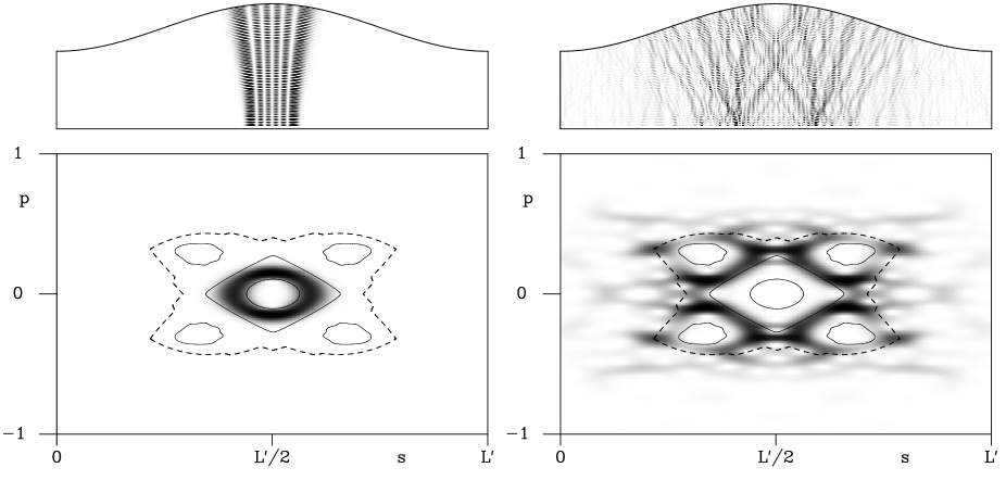
FIG. 4.: Eigenfunctions (top row) and Husimi representations (bottom row) of a regular state ($5686^{-}$, left) and a hierarchical state ($5720^{-}$, right) corresponding to the scattering states of Fig. 3.

We present in Fig. 4 the two eigenstates corresponding to the scattering states shown in Fig. 3. For each state, we show the eigenfunction density $|\psi_{n}({\bf q})|^{2}$ and the corresponding Husimi representation $H_{n}(s,p)$ (see e.g., [16, 17]). The state $5686^{-}$, displayed on the left of Fig. 4 differs in energy by about $0.01\Delta$ from the sharpest observed resonance with energy 2029.172. Note that this energy difference is of the order of the accuracy to which our resonance energies and eigenvalues are calculated. On the right hand side of Fig. 4, a hierarchical state is displayed. Its energy differs from the resonance at energy 2041.109 by about $0.1\Delta$. This shift of the resonance energy from the eigenenergy of the closed system is due to the opening of the system by attaching the leads. As for the scattering states, we have superimposed some KAM-tori onto the Husimi representations of Fig. 4. In addition, a partial transport barrier surrounding the island hierarchy is shown (see next section).

Now we want to associate all resonances of the scattering system with width $\Gamma$ at energy $E_{\rm res}$ with an eigenstate of the closed billiard with energy $E_{\rm ev}$. We use a Husimi representation $H_{n}(s,p)$ on the Poincaré section to determine the region on which an eigenstate localizes. We introduce the quantity

$$\eta_{n}=\int_{-W}^{0}ds\int_{-1}^{1}dp\,H_{n}(s,p),$$ (6)

which integrates the Husimi distribution over the left boundary of the billiard (not shown in Fig. 4) with the normalization of the Husimi distribution chosen such that $\int_{-W}^{L^{\prime}/2}ds\int_{-1}^{1}dp\,H_{n}(s,p)=1$. This quantity gives an estimate on how strongly a state of the closed system will couple to the leads in the scattering system and should be roughly proportional to $\Gamma$. This allowed us to find, for each of the 54 resonances with $\Gamma\leq\Delta/2$, a state with $E_{\rm ev}\approx E_{\rm res}$ and with $\eta\approx\Gamma$. Figures 5 and 6 show the difference $E_{\rm ev}-E_{\rm res}$ in units of the mean level spacing $\Delta$ and the approximate proportionality of $\eta$ and $\Gamma$, respectively. Clearly the larger differences appear for bigger $\Gamma$, but still a clear identification is possible (see section VI). This assignment also works the other way around, as of the 46 eigenstates with the smallest values of $\eta$, we can identify 40 with isolated resonances, missing only the 6 regular eigenstates quantized most deeply in the central island of phase space, as discussed below.

FIG. 5.: Difference of eigenstate energy $E_{\rm ev}$ and resonance energy $E_{\rm res}$ in units of the mean level spacing $\Delta$ vs $\Gamma/\Delta$. The deviations increase with $\Gamma$.

FIG. 6.: The strength $\eta$ of an eigenstate at the left boundary vs the resonance width $\Gamma$ of the corresponding resonance. An approximate proportionality can be seen.

For the 54 resonances with width $\Gamma$ less than half a mean level spacing, we analyze the structure of the corresponding eigenstates. We find that 17 states can be categorized as regular states, as their Husimi representations live inside the five major stable islands in phase space. Of these states, 7 are associated with the I-shaped orbit and 10 with the M-shaped orbit. While we observe all states in the energy interval associated with the M-shaped orbit, 6 further eigenstates living near the center of the central stability island are not resolved as resonances. As these are the innermost states in the island, we expect them to couple weaker to the leads and their resonance widths to be much smaller than the sharpest observed resonance. Apparently, these resonances are so narrow that we were not able to find them, given our current numerical accuracy, even knowing their approximate energy from the eigenvalues.

The remaining 37 resonances are not related to regular states, but the Husimi representations of their corresponding eigenstates have large intensity in the region between the regular islands and the partial transport barrier and a much weaker intensity in the rest of the chaotic region. It should be noted that in the studied energy range accessible to our methods the wave length is of the order of the distance between regular islands and the partial transport barrier. Therefore the eigenstates either look like regular states living outside the island [18] or similar to scarred states on a hyperbolic orbit close to the island [19]. For higher energies they would show the true properties of hierarchical states, i.e., being similar to a chaotic state, but restricted to the hierarchical region [14]. We therefore classify these states as hierarchical states.

In Fig. 2 we have labeled the resonances by $r$ and $h$ according to our classification of the corresponding eigenstates as regular and hierarchical, respectively. This demonstrates that the origin of all isolated resonances are hierarchical or regular eigenstates of the closed system.

V Partial transport barriers

Classical transport in the chaotic part of phase space is dominated by partial barriers [20, 21, 22, 23, 24]. They are formed by cantori as well as by stable and unstable manifolds. Such a partial transport barrier coincides with its iterate, with the exception of so-called turnstiles where phase-space volume is exchanged between both sides of the partial barrier. We have constructed partial barriers using the methods described in Ref. [20]. The fluxes $\Phi$ are determined from the length $l$ of the maximizing and minimax orbits, according to

$$\Phi = \hbar k_{F}|l_{\rm maximizing}-l_{\rm minimax}|$$ (7)

$$= \hbar\pi\sqrt{E}|l_{\rm maximizing}-l_{\rm minimax}|/W.$$ (8)

Quantum mechanically, partial transport barriers with fluxes up to the order of $\hbar$ divide the chaotic part of phase space into distinct regions with chaotic and hierarchical eigenfunctions living mainly on one or the other side [14]. We found that the partial barrier with smallest flux that surrounds the main island and the 4 neighboring islands can be constructed from the stable and unstable manifolds of the period 4 hyperbolic fixed points. Each of its two turnstiles has for our largest energy $E=2100$ a flux $1.06\hbar$. Further outside are many other partial barriers with only slightly bigger fluxes. As an example, we show in Figs. 3 and  4 the partial barrier constructed from an unstable periodic orbit with winding number $5/23$, which is an approximant of the most noble irrational between winding numbers $1/4$ and $1/5$. It has a flux $1.65\hbar$.

A check on the validity of our identification of regular and hierarchical states is provided by a comparison of their numbers to the corresponding relative volumes in phase space. To this end, we calculate the volume of the tori associated with stable periodic orbits, $V_{r}$, and the chaotic phase-space volume inside the partial transport barrier, $V_{h}$. We find $V_{r}$ and $V_{h}$ to cover 5.9% and 8.5 % of the energy shell, respectively. From the total number of eigenstates in the energy interval, $N=426$, we get for 23 (17+6) regular and 37 hierarchical states relative fractions of 5.4% and 8.7%, respectively, in good agreement with the volumes of the associated regions in phase space.

The absence of fractal conductance fluctuations in this system has now a clear explanation: According to Ref. [13] for fractal fluctuations to occur a hierarchy of partial transport barriers with fluxes larger than $\hbar$ must exist. For the studied energies we find that even the outermost partial barriers surrounding the hierarchical phase-space structure have fluxes of the order of $\hbar$. This causes a quantum dynamical decoupling of the chaotic part connected to the leads from the entire hierarchical part. As the hierarchical region is the semiclassical origin of fractal fluctuations, they are not observed. For much higher energies only, the hierarchy of partial transport barriers would have an outer region with fluxes larger than $\hbar$, leading to fractal conductance fluctuations. The inner region of this hierarchy with fluxes smaller than $\hbar$ has now a smaller phase-space volume. Still, together with the regular regions it will cause isolated resonances on smaller scales than the fractal fluctuations. Unfortunately, this energy regime is currently computationally inaccessible for the studied system.

Power laws in the distribution of resonance widths and in the variance of conductance increments had been observed in Ref. [11], apparently reflecting the classical dwell time exponent. They were related to the resonances below the mean level spacing. For these resonances we now have demonstrated that they arise due to hierarchical and regular states. This allows to apply the arguments of Ref. [13] about the resonance width distribution of hierarchical states. They lead to the conclusion that these apparent power laws come from broad transition regions to asymptotic distributions that are unrelated to the classical dwell time exponent.

VI Avoided crossings

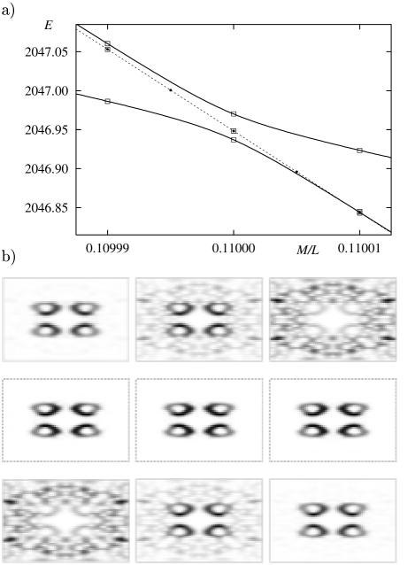
FIG. 7.: (a) Energies of states $5736^{-}$ and $5737^{-}$ (solid lines) showing an avoided crossing under variation of $M/L$. The energy of the only isolated resonance in this energy range (dots connected by a dashed line) follows the regular state of the closed system. The slight offset in the resonance energy is within the systematic numerical error of the numerical method. (b) The Husimi representations for state $5737^{-}$ (top row), the scattering state (middle row) and for eigenstate $5736^{-}$ (bottom row) are shown for $M/L=0.10999,\,0.11,\,0.11001$ (left to right). For the eigenstates one clearly sees the typical exchange of the structure while passing the avoided crossing whereas the scattering state is not affected.

While for most resonances and corresponding eigenstates the parameters $\eta$ and $\Gamma$ are of the same order of magnitude, for some states $\eta$ exceeds $\Gamma$ by up to 2 orders of magnitude. This phenomenon can be understood as an effect of avoided level crossings in the closed system: In Fig. 7a) we show as an example the dependence of the energy of states $5736^{-}$ and $5737^{-}$ as a function of the parameter $M/L$ for the narrow range $0.10999\leq M/L\leq 0.11001$, displaying the typical features of an avoided crossing. A comparison of the associated Husimi representations shows that the states $5736^{-}$ and $5737^{-}$ do indeed exchange their character from chaotic to regular and from regular to chaotic, respectively, showing a superposition at $M/L=0.11$. Upon opening the system, the chaotic state couples much more strongly to the leads as compared to the regular one. Consequently, in the complex energy plane of the scattering system there is no longer an avoided crossing. The regular state leads to an isolated resonance with an almost linear energy dependence on $M/L$ and the phase-space signature of the regular state (middle row in Fig. 7b). It closely follows the expected energy dependence of the regular state in the closed system if it had not made an avoided crossing with the chaotic state (Fig. 7a).

Another example of an avoided crossing is given by state $5801^{-}$ with an eigenvalue about $0.5\Delta$ less than the resonance position (see lower right corner of Fig. 5) and the state $5802^{-}$, with an eigenenergy about $1.4\Delta$ above the resonance energy. Both states show similar Husimi representations and have $\eta$ values exceeding $\Gamma$ by about a factor of ten.

In all the cases when $\eta$ drastically exceeds $\Gamma$ a closer look at these eigenstates reveals that they are superpositions of regular or hierarchical states with chaotic states. They are due to avoided crossings and the chaotic part leads to a comparatively large value of $\eta$. In contrast, in the open system no avoided crossing occurs in the complex energy plane and the resonance width $\Gamma$ is unaffected.

VII Conclusion and Outlook

We demonstrate a clear correspondence of the isolated resonances observed in the transport properties of the open cosine billiard to hierarchical and regular eigenstates of the closed billiard. We can identify all resonances with widths less than half of the mean level spacing. The classification of resonances into a hierarchical or regular origin yields numbers in agreement with the relative phase-space volumes. On a quantitative level, we find a roughly linear relation between the widths of the isolated resonances and the weights of the associated eigenstates at the part of the boundary where the leads are attached. States with unusually large weights can be attributed to avoided crossings with chaotic eigenstates.

We find that the island hierarchy is separated from the chaotic part of phase space by partial transport barriers with fluxes of the order of $\hbar$. This supports the notion that the absence of fractal conductance fluctuations in the currently accessible energy range is due to the quantum dynamical decoupling of the hierarchical part of phase space from the chaotic part connected to the external leads.

The simultaneous appearance of isolated resonances and fractal fluctuations, beyond the quantum graph model studied in Ref. [13], remains to be demonstrated numerically or experimentally for a system with a mixed phase space. Numerically, the challenge is the observation of fractal fluctuations of the conductance, which go beyond one order of magnitude [25]. This requires calculations with a drastically increased number of modes, the use of improved techniques like the modular recursive Green’s function method [26], and the search for suitable billiard systems where the turnstile fluxes across partial barriers are particularly large. Isolated resonances will easily appear as soon as the parameter is varied on a sufficiently small scale. We note, that fluctuations of the quantum staying probability, which can be fractal [8], cannot show isolated resonances. Similarly, we expect no appearance of isolated resonances within the fractal fluctuations observed in recent studies [27], as they are unrelated to a classical mixed phase space.

On the experimental side, fractal conductance fluctuations have been observed [6, 7] and also isolated resonances coming from regular regions have been recently reported [28]. The simultaneous appearance of both types including isolated resonances from hierarchical regions requires to go far enough into the semiclassical regime, i.e. to quantum dots with dimensions bigger than 1 $\mu$m, as in Ref. [6]. At the same time the phase coherence time must be large enough to resolve isolated resonances of a given width and, of course, the parameter, typically a magnetic field, must be varied on a sufficiently fine scale. Given the experimental limitations it would be helpful if an optimal form for such a quantum dot could be provided by theoretical considerations. This seems to be quite difficult at present, since the difference in the lithographic shape and the actual potential experienced by electrons has dramatic consequences on the electron dynamics and thus on the scales over which fractal fluctuations and isolated resonances appear.

Acknowledgments

R.K. acknowledges helpful discussions with L. Hufnagel and M. Weiss. A.B. acknowledges support by the Deutsche Forschungsgemeinschaft under contract No. DFG-Ba 1973/1-1.

A Hybrid representation and recursive Green function method

In this appendix we discuss the numerical method to determine the scattering matrix $S$ and the time delay $\tau$. The $S$-matrix of a symmetric scattering system can be expressed in terms of the Green function $G$

$$S = \left(\begin{array}[]{cc}r&t^{\prime}\\ t&r^{\prime}\end{array}\right),$$ (A3)

$$t^{\prime} = t^{T},$$ (A4)

$$r^{\prime} = r,$$ (A5)

$$t_{\alpha\beta} = -i\hbar\sqrt{v_{\alpha}v_{\beta}}G_{\alpha\beta}(0,L),$$ (A6)

$$r_{\alpha\beta} = \delta_{\alpha\beta}-i\sqrt{v_{\alpha}v_{\beta}}G_{\alpha\beta}(0,0),$$ (A7)

where

$$v_{\alpha}=\left(\frac{2}{m}\left(E-\frac{\hbar^{2}}{2mW^{2}}\alpha^{2}\pi^{2}\right)\right)^{1/2},$$ (A8)

is the velocity of mode $\alpha$ and

$$G_{\alpha\beta}(x,x^{\prime})=\int_{x}dy\int_{x^{\prime}}dy^{\prime}\phi^{*}_{\alpha}(y;x)\phi_{\beta}(y^{\prime};x^{\prime})G^{+}({\bf r},{\bf r}^{\prime};E)$$ (A9)

is the projection of the retarded Green function $G^{+}({\bf r},{\bf r}^{\prime};E)$ onto the local transverse modes

$$\phi_{\alpha}(y;x)=\sqrt{\frac{2}{W(x)}}\sin\left(\frac{\alpha\pi y}{W(x)}\right).$$ (A10)

The Green function can be calculated recursively. Expanding the Hamiltonian

$$H=\frac{\hbar^{2}}{2m}\left(\frac{\partial^{2}}{\partial x^{2}}+\frac{\partial^{2}}{\partial y^{2}}\right)$$ (A11)

in terms of the local transverse modes (A10) and discretizing in $x$ direction with a lattice constant $a$, $x=ma$, we obtain the Hamiltonian in hybrid representation [29]

$$H_{h} = \sum_{\alpha,m}|\alpha,m\rangle\left(\epsilon^{\alpha}_{m}+2E_{t}\right)\langle\alpha,m|$$ (A14)

$$-\sum_{\alpha,\beta,m}\left(t^{\alpha\beta}_{m,m+1}|\alpha,m\rangle\langle\beta,m+1|\right.$$

$$\left.+t^{\alpha\beta}_{m+1,m}|\alpha,m+1\rangle\langle\beta,m|\right),$$

with

$$\epsilon^{\alpha}_{m} = \left(\alpha\frac{a}{W(ma)}\right)^{2},$$ (A15)

$$t^{\alpha\beta}_{m,m+1} = E_{t}\int\phi^{*}_{\alpha}(y;ma)\phi_{\beta}(y;(m+1)a)dy,$$ (A16)

and $E_{t}=\hbar^{2}/(2ma^{2})$. In order to recursively calculate the Green function associated with $H_{h}$, we split the Hamiltonian $H_{h}^{M+1}$ of a system with $m=1,\ldots,M+1$ into two parts,

$$H_{h}^{M+1} = H_{0}+U,$$ (A17)

$$H_{0} = H_{h}^{M}+$$ (A19)

$$\sum_{\alpha}|\alpha,M+1\rangle\left(\epsilon^{\alpha}_{M+1}+2E_{t}\right)\langle\alpha,M+1|,$$

$$U = -\sum_{\alpha,\beta}\left(t^{\alpha\beta}_{M,M+1}|\alpha,M\rangle\langle\beta,M+1|\right.$$ (A21)

$$\left.+t^{\alpha\beta}_{M+1,M}|\alpha,M+1\rangle\langle\beta,M|\right).$$

Dyson’s equation,

$$G^{M+1}=G_{0}+G_{0}UG^{M+1},$$ (A22)

then allows to calculate the Green function $G^{M+1}$ of $H_{h}^{M+1}$ from $G^{M}$ and

$$G_{0} = \left(E-H_{0}\right)^{-1}$$ (A23)

$$= G^{M}+\sum_{\alpha}|\alpha,M+1\rangle g_{0}^{M+1}\langle\alpha,M+1|,$$ (A24)

$$g_{0}^{M+1} = \left(E-\epsilon^{\alpha}_{M+1}-2E_{t}\right)^{-1}.$$ (A25)

We start the recursion with $M=1$ at the left edge of the closed billiard and iterate to the right edge at $M=N_{L}=L/a$. In order to attach the leads, we again split the Hamiltonian according to eq. (A17), but this time $H_{0}$ contains the Hamiltonian of the closed billiard and the semi-infinite leads. In the leads, $\epsilon^{\alpha}_{m}=(\alpha a/W)^{2}$ and $t^{\alpha\beta}_{m,m+1}=\delta_{\alpha\beta}E_{t}$. $U$ is the coupling between the billiard and the semi-infinite leads. The Green function for the leads is known analytically [30].

The recursion scheme is exact for an infinite number $N_{L}$ of slices and an infinite number $N_{C}$ of transverse modes. For numerical calculations, both numbers have to be kept finite. We find that the deviations from the asymptotic values for, e.g., the width $\Gamma$ of a resonance scale as

$$\Gamma(N_{C},N_{L})=\Gamma+bN_{C}^{-4}+cN_{L}^{-2},$$ (A26)

with positive numerical coefficients $b$ and $c$. For our choice of parameters, $N=45$ transmitting modes in the leads, the values $N_{C}=108$ and $N_{L}=12000$ give an accuracy of about $1\%$ for the resonance width. The corrections to the position of the resonance have the same functional form as in eq. (A26), however, they can be either positive or negative, depending on the values of $N_{C}$ and $N_{L}$. This explains the slight offset of the resonance energies with respect to the eigenenergies of the closed system seen in Fig. 7a).

REFERENCES

- [1] R. A. Jalabert, in: Proceedings of the International School of Physics “Enrico Fermi”, Course CXLIII New Directions in Quantum Chaos, G. Casati, I. Guarneri and U. Smilansky (eds.), IOS Press Amsterdam (2000).
- [2] A. J. Lichtenberg and M. A. Liebermann, Regular and chaotic dynamics,, 2nd ed. (Springer-Verlag, New York, 1992).
- [3] B. V. Chirikov and D. L. Shepelyansky, in Proceedings of the IXth Intern. Conf. on Nonlinear Oscillations, Kiev, 1981 [Naukova Dumka 2, 420 (1984)] (English Translation: Princeton University Report No. PPPL-TRANS-133, 1983); C. F. F. Karney, Physica 8 D, 360 (1983); B. V. Chirikov and D. L. Shepelyansky, Physica 13 D, 395 (1984); P. Grassberger and H. Kantz, Phys. Lett. 113 A, 167 (1985); Y. C. Lai, M. Ding, C. Grebogi, and R. Blümel, Phys. Rev. A 46, 4661 (1992).
- [4] Y.-C. Lai, R. Blümel, E. Ott, and C. Grebogi, Phys. Rev. Lett. 68, 3491 (1992).
- [5] R. Ketzmerick, Phys. Rev. B 54, 10841 (1996).
- [6] A. S. Sachrajda et al., Phys. Rev. Lett. 80, 1948 (1998).
- [7] A. P. Micolich et.al., Phys. Rev. Lett. 87, 036802 (2001).
- [8] G. Casati, I. Guarneri, and G. Maspero, Phys. Rev. Lett. 84, 63 (2000).
- [9] P. Stifter, Diploma thesis, Universität Ulm, 1993 (unpublished); P. Stifter, Ph. D. thesis, Universität Ulm, 1996 (unpublished).
- [10] G. A. Luna-Acosta et al., Phys. Rev. B 54, 11410 (1996); A. Bäcker, R. Schubert, and P. Stifter, J. Phys. A: Math. Gen. 30, 6783 (1997).
- [11] B. Huckestein, R. Ketzmerick, and C. H. Lewenkopf, Phys. Rev. Lett. 84, 5504 (2000), erratum: Phys. Rev. Lett. 87, 119901(E) (2001).
- [12] P. Šeba, Phys. Rev. E 47, 3870 (1993).
- [13] L. Hufnagel, M. Weiss, and R. Ketzmerick, Europhys. Lett. 54, 703 (2001).
- [14] R. Ketzmerick, L. Hufnagel, F. Steinbach, and M. Weiss, Phys. Rev. Lett. 85, 1214 (2000).
- [15] A. Bäcker, contribution to the Proceedings of the Summer School The Mathematical Aspects of Quantum Chaos I, Bologna, 2001, to be published (2002).
- [16] J. M. Tualle and A. Voros, Chaos, Solitons and Fractals 5, 1085 (1995).
- [17] F. P. Simonotti, E. Vergini, and M. Saraceno, Phys. Rev. E 56, 3859 (1997).
- [18] O. Bohigas, S. Tomsovic, and D. Ullmo, Phys. Rep. 223, 43 (1993).
- [19] G. Radons and R. E. Prange, Phys. Rev. Lett. 61 (1988) 1691. G. Radons and R. E. Prange, in: Quantum chaos (Trieste, 1990), 333, World Sci. Publishing, River Edge, NJ, (1991).
- [20] R. S. MacKay, J. D. Meiss, and I. C. Percival, Physica D 13, 55 (1984).
- [21] J. D. Hanson, J. R. Cary, and J. D. Meiss, J. Statist. Phys. 39, 327 (1985).
- [22] J. D. Meiss and E. Ott, Physica D 20, 387 (1986).
- [23] T. Geisel, A. Zacherl, and G. Radons, Phys. Rev. Lett. 59, 2503 (1987).
- [24] J. Meiss, Rev. Mod. Phys. 64, 795 (1992).
- [25] Y. Takagaki and K. H. Ploog, Phys. Rev. B 61, 4457 (2000).
- [26] S. Rotter et al., Phys. Rev. B 62, 1950 (2000).
- [27] E. Louis and J. A. Verges, Phys. Rev. B 61, 13014 (2000); G. Benenti, G. Casati, I. Guarneri, and M. Terraneo, Phys. Rev. Lett. 87, 014101 (2001); I. Guarneri and M. Terraneo, Phys. Rev. E 65, 015203(R) (2001).
- [28] A. P. S. de Moura et al., to be published.
- [29] F. A. Maaø, I. V. Zozulenko, and E. H. Hauge, Phys. Rev. B 50, 17320 (1994).
- [30] E. N. Economou: Green’s Functions in Quantum Physics. No. 7 in Solid-State Sciences. Springer-Verlag, 2nd edition (1990).