Abstract

The time evolution of several interacting Ginzburg-Landau vortices according to an equation of Schrödinger type is approximated by motion on a finite-dimensional manifold. That manifold is defined as an unstable manifold of an auxiliary dynamical system, namely the gradient flow of the Ginzburg-Landau energy functional. For two vortices the relevant unstable manifold is constructed numerically and the induced dynamics is computed. The resulting model provides a complete picture of the vortex motion for arbitrary vortex separation, including well-separated and nearly coincident vortices.

AMS classification scheme numbers: 35Q55, 37K05, 70K99

1 Ginzburg-Landau vortices and their dynamics

Vortices play a fundamental role in a large variety of physical systems, ranging from ordinary fluids over condensed matter to the early universe. This variety is reflected in the mathematical models used to describe the formation, structure and dynamics of vortices. In fluid dynamics, the basic ingredient of the mathematical model is the velocity field of the fluid, and the vortex is a particular configuration of that velocity field. In condensed matter theory, the mathematical models are field theories. The basic field of such models is a complex valued scalar field, and vortices are particular configurations of that field. One important difference between vortices in ordinary fluids and those in condensed matter systems is that the total vorticity can take arbitrary real values in the former but is quantised in the latter. Nonetheless, it is sometimes possible to establish a precise mathematical connection between field theory models and those used in ordinary fluid dynamics.

In this paper we are concerned with vortices in the Ginzburg-Landau model. For general background and references we refer the reader to the book [1]. We are interested in the dynamics of such vortices in the plane, so the basic field of the model is the function

$$\psi:\mathbb{R}\times\mathbb{R}^{2}\rightarrow\mathbb{C},$$ (1.1)

depending on time $t\in\mathbb{R}$ and spatial coordinates $x=(x_{1},x_{2})\in\mathbb{R}^{2}$. Sometimes we also use polar coordinates $(r,\theta)$ in the plane and parametrise the field $\psi$ in terms of its argument and modulus via $\psi=\sqrt{\rho}\exp(i\phi)$, where $\rho=|\psi|^{2}$. In this paper $\psi$ will be used to denote both time-dependent and static configurations. For static configurations we often suppress the first argument and simply write $\psi(x)$. For configurations varying with time we sometimes write $\dot{\psi}$ for the partial derivative $\partial_{t}\psi$. Often we write $\partial_{1}$ for $\partial/\partial x_{1}$, $\partial_{t}$ for $\partial/\partial t$ and so on.

The Ginzburg-Landau energy is the following functional of $\psi$:

$$E[\psi]=\frac{1}{2}\int{\nabla\psi}\nabla\bar{\psi}+\frac{1}{2}(|\psi|^{2}-1)^{2}\,d^{2}x.$$ (1.2)

We impose the boundary condition

$$\lim_{r\rightarrow\infty}|\psi(r,\theta)|=1,$$ (1.3)

which implies that for sufficiently large $R$ the field

$$\psi_{R}(\theta)=\frac{\psi}{|\psi|}(R,\theta)$$ (1.4)

is a well-defined map from the spatial circle of large radius $R$ to the unit circle in $\mathbb{C}$. It therefore has an associated integer winding number or degree, which can be computed via the following line integral over the circle $S^{1}_{R}$ of radius $R$

$$\mbox{deg}[\psi]=\frac{1}{2\pi i}\oint_{S^{1}_{R}}d\ln\psi.$$ (1.5)

This integer, denoted $n$ in the following, is also called the vortex number.

The variational derivative of the Ginzburg-Landau functional (1.2) with respect to $\bar{\psi}$ is

$$\frac{\delta E}{\delta\bar{\psi}}=-\frac{1}{2}\left(\Delta\psi+(1-|\psi|^{2})\psi\right)$$ (1.6)

and, because of the reality of $E$,

$$\frac{\delta E}{\delta{\psi}}=\overline{\frac{\delta E}{\delta\bar{\psi}}}.$$ (1.7)

The Ginzburg-Landau equation is the equation for critical points of the Ginzburg-Landau energy, so it reads

$$-\Delta\psi+(|\psi|^{2}-1)\psi=0.$$ (1.8)

A Ginzburg-Landau vortex is a solution of this equation with non-vanishing vortex number $n$. It is shown in [2] that for any configuration of non-vanishing vortex number which attains the limit (1.3) uniformly in $\theta$ the Ginzburg-Landau energy is necessarily infinite. The origin of this divergence is not difficult to understand and also explained in [2]. The essential point is that the gradient terms in the energy density contain the term $|\partial_{\theta}\psi|^{2}/r^{2}$ which, for $n\neq 0$, leads to a logarithmic divergence. Since the divergence only depends on $n$ and not on any other details of the configuration, it can be removed by introducing a smooth cut-off function

$$\chi_{R}(x)=\left\{\begin{array}[]{cl}0&\,\,\mbox{for}\,\,|x|\leq R\\ 1&\,\,\mbox{for}\,\,|x|\geq R+R^{-1}\end{array}\right.$$ (1.11)

and defining the renormalised energy functional

$$E_{\mbox{\tiny ren}}[\psi]=\frac{1}{2}\int{\nabla\psi}\nabla\bar{\psi}-\frac{\mbox{deg}[\psi]^{2}}{r^{2}}\chi_{R}+\frac{1}{2}(|\psi|^{2}-1)^{2}\,d^{2}x.$$ (1.12)

This renormalisation procedure is natural both from the point of view of physics and in numerical investigations. The point is that the total vortex number $n$ is conserved during the time evolution. When studying the interacting dynamics of $n$ vortices during a finite time interval we can choose $R$ so large that all the vortices remain well inside the disc of radius $R$ during that time interval. The renormalisation procedure removes a divergence which only depends on the conserved quantity $n$ but not on any other details of the dynamics.

In studying the dynamics of vortices one has a choice of several different ways of extending the static Ginzburg-Landau equation to a time-dependent evolution equation. We are interested in the following first-order equation of Schrödinger type, often called the Gross-Pitaevski equation:

$$i\frac{\partial\psi}{\partial t}=-\Delta\psi+(|\psi|^{2}-1)\psi.$$ (1.13)

The vortex dynamics dictated by this equation has been studied in a large number of publications. In two seminal papers [3, 4] Neu showed that in a scaling limit where the vortex size shrinks to zero, the time evolution according to the partial differential equation (1.13) reduces to a set of coupled ordinary differential equation for the centres of vorticity. Moreover, he showed that set of ordinary equations to be the Kirchhoff-Onsager law for the motion of fluid vortices in incompressible, nonviscous two-dimensional flows. Neu’s work has in turn inspired a number of authors. Some, mathematically motivated, have investigated the scaling limit further and have put his work on a more rigorous mathematical footing, see [5, 6] and [7]. Others, starting with the interpretation of Neu’s work as a finite-dimensional approximation to the infinite-dimensional dynamical system governed by the Gross-Pitaevski equation, have tried to go beyond this approximation. Physically, one may think of Neu’s approximation as a point-particle approximation to vortex dynamics in a field theory. This approximation is expected to be reasonable when the vortices are well-separated and moving slowly. However, when the vortices overlap, the point-particle approximation is poor. Similarly, when the vortices move rapidly we expect them to excite radiation in the field theory which is not captured by the point-particle approximation.

More recently, Ovchinnikov and Sigal have derived Neu’s approximation from a different point of view and have computed leading radiative corrections to it in a series of papers [8, 9]. They work with the Lagrangian from which the Gross-Pitaevski equation can be derived and explicitly study the truncation of the infinite dimensional Gross-Pitaevski dynamical system to a finite-dimensional family of multi-vortex configurations with pinned centres of vorticity. The induced Lagrangian on that finite dimensional family reproduces the Kirchoff-Onsager law when the vortex centres are well-separated. Moreover, the approach makes it possible to study the coupling between the vortex motion and radiative modes and to compute radiative corrections. However, Ovchinnikov and Sigal’s family of pinned multi-vortex configurations is less useful when trying to understand the dynamics of overlapping vortices. When vortices get close together pinning the vortex centres is mathematically awkward and physically unnatural. In this paper we study the truncation of the Gross-Pitaevski dynamical system to a finite dimensional dynamical system using a different set of multi-vortex configurations. Our configurations are similar to those of Ovchinnikov and Sigal when the vortices are well-separated, but we believe they provide a more accurate description of vortex dynamics when the vortices overlap. Our approach is inspired by an approximation scheme proposed by Manton [10] in the context of Lagrangian soliton dynamics. Manton considered the problem of defining a smooth finite-dimensional family of multi-soliton configurations which could be used as the configuration space for a finite-dimensional low-energy approximation to multi-soliton dynamics. His proposal is to consider an auxiliary evolution equation, namely the gradient flow in the potential energy functional, and to use the unstable manifold of a suitable saddle point as the truncated configuration space. Such an unstable manifold is the union of paths of steepest descent from the saddle point. In practice this scheme is not easy to implement, and so far it has only been used to study soliton dynamics in one spatial dimension [11]. In this paper we show that it is very well suited to studying the dynamics of overlapping Ginzburg-Landau vortices. The basic reason is that in the Ginzburg-Landau model there are well-known rotationally symmetric saddle point solutions for all vortex numbers $|n|>1$ which can be used for the construction of the unstable manifold. We focus on the case $n=2$ and find that the relevant unstable manifold is two-dimensional. We describe its geometry, compute the induced Lagrangian and use it to study the relative motion of two vortices at arbitrary separation.

2 The Gross-Pitaevski equation and its symmetries

For our study of the Gross-Pitaevski equation it is essential that we can derive it from a Lagrangian. The required Lagrangian is the following functional of time-dependent fields $\psi$

$$L[\psi]=T[\psi,\dot{\psi}]-E[\psi],$$ (2.1)

where the kinetic energy functional $T$ is given by

$$T(\psi,\dot{\psi})=-\frac{1}{2}\int\mbox{Im}(\bar{\psi}\dot{\psi})\,d^{2}x$$ (2.2)

and the potential energy functional $E$ is the Ginzburg-Landau functional (1.2). One checks that, essentially because of the linearity of the kinetic energy in $\dot{\psi}$, the total energy or Hamiltonian is equal to the potential energy $E$. Using the formula (1.6), the Euler-Lagrange equation of $L$

$$\partial_{t}\psi=-2i\frac{\delta E}{\delta\bar{\psi}},$$ (2.3)

is readily seen to be the Gross-Pitaevski equation (1.13).

We define the configuration space to be the space of smooth fields $\psi$ satisfying the boundary condition (1.3), i.e.

$${\cal C}=\{\psi:\mathbb{R}^{2}\rightarrow\mathbb{C}|\lim_{|x|\rightarrow\infty}|\psi(x)|=1\}.$$ (2.4)

As mentioned earlier, the boundary condition means that every $\psi\in{\cal C}$ has an associated integer winding number or degree. Using Stokes’s theorem and taking the radius $R$ to infinity in (1.5) one shows that the degree can also be written as the integral

$$\mbox{deg}[\psi]=\int_{\mathbb{R}^{2}}\gamma,$$ (2.5)

where the integrand

$$\gamma=\frac{1}{2\pi i}d\bar{\psi}\wedge d\psi$$ (2.6)

is called the vorticity. The integer degree cannot change under the continuous time evolution, which can therefore be restricted to one of the topological sectors

$${\cal C}_{n}=\{\psi\in{\cal C}|\,\mbox{deg}[\psi]=n\}.$$ (2.7)

For each $n$, the pair $({\cal C}_{n},L)$ is an infinite dimensional Lagrangian dynamical system. From the Lagrangian viewpoint ${\cal C}_{n}$ is the configuration space and a motion is a path $t\mapsto\psi(t,\cdot)$ in ${\cal C}_{n}$ which satisfies the evolution equation (1.13). Alternatively, we can adopt the Hamiltonian point of view. Then ${\cal C}_{n}$ should be thought of as the phase space and the kinetic part of the Lagrangian (2.1) defines a symplectic structure on ${\cal C}_{n}$. This is a two-form $\Omega$ on the tangent space of ${\cal C}_{n}$. For a more careful discussion of that tangent space we refer the reader to [2], but for our purpose it is sufficient to think of tangent vectors as complex valued functions which tend to zero at infinity. If $\xi$ is such a tangent vector we use the notation introduced in [2] for elements of the complexified tangent space:

$$\vec{\xi}=\pmatrix{\xi\cr\bar{\xi}}.$$ (2.8)

If $\xi$ and $\eta$ are two elements of the same tangent space the symplectic form is defined via

$$\Omega(\vec{\xi},\vec{\eta})=\frac{1}{2i}\int(\xi\bar{\eta}-\bar{\xi}\eta)\,d^{2}x.$$ (2.9)

It follows that the Poisson bracket of $\psi$ and $\bar{\psi}$ is

$$\{\psi,\bar{\psi}\}=2i.$$ (2.10)

One checks that the Gross-Pitaevski equation can then be written in the canonical form

$$\dot{\psi}=\{E[\psi],\psi\}.$$ (2.11)

As an aside we point out that the total vorticity or degree is related to the pull-back of the symplectic form $\Omega$ evaluated on the vector fields $\partial_{1}$ and $\partial_{2}$ on $\mathbb{R}^{2}$ :

$$\psi^{*}\Omega(\partial_{1},\partial_{2})=-\pi\int_{\mathbb{R}^{2}}\gamma.$$ (2.12)

Thus if $\psi\in{\cal C}_{n}$ then $\psi^{*}\Omega(\partial_{1},\partial_{2})=-n\pi$.

The Lagrangian $L$ has a large invariance group. Writing $R\in SO(2)$ for spatial rotations and $d\in\mathbb{R}^{2}$ for translations in the plane, elements $(R,d)$ of the Euclidean group

$$E_{2}=SO(2)\ltimes\mathbb{R}^{2}$$ (2.13)

act on fields via pull-back

$$\psi\mapsto\psi\circ(R,d)^{-1},$$ (2.14)

i.e. $\psi\circ(R,d)^{-1}(x)=\psi(R^{-1}(x-d))$. Both the Lagrangian and the degree are invariant under this action. Similarly, unit complex numbers $e^{i\alpha}\in U(1)$ act on fields $\psi$ as phase rotations

$$\psi\mapsto e^{i\alpha}\psi$$ (2.15)

and leave both the Lagrangian and the degree invariant. Spatial reflections about any axis leave the Lagrangian invariant but change the sign of the degree. The same is true for the combination of complex conjugation with time reversal $T:t\mapsto-t$ . However, with $S:(x_{1},x_{2})\mapsto(x_{1},-x_{2})$, the combination

$$C:\psi\mapsto\bar{\psi}\circ(ST)$$ (2.16)

leaves the degree and the Lagrangian invariant. To sum up, for each $n\in\mathbb{Z}$ the group

$$C\ltimes\left(E_{2}\times U(1)\right)$$ (2.17)

acts on ${\cal C}_{n}$ preserving the Lagrangian $L$ and hence the equations of motion. The two-dimensional Galilean group provides an additional more subtle symmetry. If $\psi(t,x)$ solves the Gross-Pitaevski equation, then so does the configuration

$$\psi_{v}(t,x)=e^{i(\frac{1}{2}x\cdot v-\frac{1}{4}v^{2}t)}\psi(t,x-vt),$$ (2.18)

where the parameter $v\in\mathbb{R}^{2}$ is physically interpreted as the boost velocity.

To end this section we note the conservation laws which follow from the symmetry group (2.17). The Noether charge which is conserved due to the invariance under phase rotations is

$$Q[\psi]=\int_{\mathbb{R}^{2}}|\psi|^{2}\,d^{2}x.$$ (2.19)

Invariance under spatial rotations leads to the conserved charge

$$J[\psi]=\int_{\mathbb{R}^{2}}\mbox{Im}(\bar{\psi}\partial_{\theta}\psi)\,d^{2}x$$ (2.20)

and invariance under translations leads to the conservation of the vector $(P_{1},P_{2})$ with components

$$P_{i}[\psi]=\int_{\mathbb{R}^{2}}\mbox{Im}(\bar{\psi}\partial_{i}\psi)\,d^{2}x\quad i=1,2.$$ (2.21)

All of the above charges have to be handled with care because the integrals defining them do not generally converge for configurations with non-vanishing degree. In [12] a related field theory was studied and it was pointed out that the Noether charges can be related to moments of the vorticity. In our cases the moments

$$\tilde{J}[\psi]=-\pi\int_{\mathbb{R}^{2}}(x_{1}^{2}+x_{2}^{2})\gamma$$ (2.22)

and

$$\tilde{P}_{1}[\psi]=2\pi\int_{\mathbb{R}^{2}}x_{2}\gamma\quad\mbox{and}\quad\tilde{P}_{2}[\psi]=-2\pi\int_{\mathbb{R}^{2}}x_{1}\gamma$$ (2.23)

are also conserved during time evolution according to (1.13) and can be obtained from the Noether charges $J$, $P_{1}$ and $P_{2}$ by integration by parts. For some configurations the integrals defining $\tilde{J}$ and $\tilde{P}_{i}$ are convergent even when those defining $J$ and $P$ are not. The Galilean symmetry also implies a conservation law, but it will not be required in this paper.

3 The $n=2$ saddle point and its unstable mode

Imposing extra symmetry is the easiest way of finding static solutions of the Ginzburg-Landau equations. The largest invariance group one can impose on configurations of degree $n$ is a group containing reflections and combinations of spatial rotations $R(\chi)$ by an angle $\chi$ with suitable phase rotations. More precisely we define the subgroup

$$R_{n}=C\ltimes\{(R(\chi),e^{in\chi})\in SO(2)\times U(1)|\chi\in[0,2\pi)\}$$ (3.1)

of the symmetry group (2.17). Configurations invariant under this group are of the form

$$\psi_{n}(r,\theta)=f_{n}(r)e^{in\theta},$$ (3.2)

where $f_{n}$ is real and satisfies the boundary condition

$$f_{n}(0)=0\quad\mbox{for}\quad n\neq 0\quad\mbox{and}\lim_{r\rightarrow\infty}f_{n}(r)=1.$$ (3.3)

The Ginzburg-Landau equation implies the following ordinary differential equation for $f_{n}$

$$\frac{1}{r}\frac{d}{dr}\left(r\frac{df_{n}}{dr}\right)-\frac{n^{2}}{r^{2}}f_{n}+(1-f_{n}^{2})f_{n}=0.$$ (3.4)

As proved for example in [1], this equation has a unique solution satisfying the boundary conditions (3.3) for each $n$, and in the following we use $f_{n}$ to denote that solution. Near $r=0$ and for large $r$ the equation can be solved approximately

$$f_{n}(r) \sim A_{n}r^{n}\quad\mbox{for small}\,r,$$

$$f_{n}(r) \sim 1-\frac{n^{2}}{2r^{2}}\quad\mbox{for large}\,r,$$ (3.5)

where $A_{n}$ are real constants. However, no exact expression for $f_{n}$ in terms of standard functions is known. For $|n|=1$ the resulting vortex configuration is a stable solution of the Ginzburg-Landau equation. For $|n|>1$ the solution is an unstable saddle point. Bounds on the number of unstable modes were derived by Ovchinnikov and Sigal in [2]. It follows from their analysis that for $n=2$ there is precisely one unstable mode. Since this mode plays an important role in our analysis, we describe and compute it explicitly. For further general background we refer the reader to [2]. The required unstable mode is an eigenvector of the Hessian of the Ginzburg-Landau energy

$$\mbox{Hess}\,E[\psi]=\pmatrix{\frac{\delta^{2}E}{\delta\psi\delta\bar{\psi}}&\frac{\delta^{2}E}{\delta\bar{\psi}^{2}}\cr\frac{\delta^{2}E}{\delta\psi^{2}}&\frac{\delta^{2}E}{\delta\psi\delta\bar{\psi}}}.$$ (3.6)

For the saddle point $\psi_{2}$ the Hessian takes the form

$$\mbox{Hess}\,E[\psi_{2}]=\frac{1}{2}\pmatrix{-\Delta+2\rho_{2}-1&\rho_{2}e^{4i\theta}\cr\rho_{2}e^{-4i\theta}&-\Delta+2\rho_{2}-1},$$ (3.7)

where $\rho_{2}=|\psi_{2}|^{2}$. In terms of the notation (2.8) the eigenvalue equation

$$2\mbox{Hess}\,E[\psi_{2}]\vec{\xi}=\lambda\vec{\xi}$$ (3.8)

is thus equivalent to

$$-\Delta\xi+(2\rho_{2}-1)\xi+\rho_{2}e^{4i\theta}\bar{\xi}=\lambda\xi,$$ (3.9)

which can also be obtained by linearising the Ginzburg-Landau equation around the saddle point $\psi_{2}$. If $\xi$ solves (3.9) then the leading term in the difference $E[\psi_{2}+\xi]-E[\psi_{2}]$ is the second order term

$$E^{(2)}(\vec{\xi}) = \frac{1}{2}\int(\vec{\xi})^{\dagger}\,\mbox{Hess}\,E[\psi_{2}]\,\vec{\xi}$$ (3.10)

$$= \frac{1}{2}\lambda\langle\vec{\xi},\vec{\xi}\rangle,$$

where we used the inner product

$$\langle\vec{\xi},\vec{\eta}\rangle=\frac{1}{2}\int(\xi\bar{\eta}+\eta\bar{\xi})\,d^{2}x.$$ (3.11)

To study the eigenvalue problem (3.9) and to compute the variation in the energy it is best to expand the $\theta$-dependence of $\xi$ into a Fourier series. The term $\rho_{2}e^{4i\theta}$ in the equation leads to a coupling between Fourier modes $e^{ik\theta}$ with $k$ differing by $4$, but all other modes decouple. As explained in [13], the unique eigenfunction with a negative eigenvalue is of the form

$$\xi(r,\theta)=u(r)+v(r)e^{4i\theta}.$$ (3.12)

Inserting this expression into (3.9) leads to coupled equations for the radial functions $u$ and $v$

$$-\frac{1}{r}\frac{d}{dr}\left(r\frac{du}{dr}\right)+\left(2\rho_{2}-1\right)u+\rho_{2}v = \lambda u$$

$$-\frac{1}{r}\frac{d}{dr}\left(r\frac{dv}{dr}\right)+\left(\frac{16}{r^{2}}+2\rho_{2}-1\right)v+\rho_{2}u = \lambda v.$$ (3.13)

In terms of $u$ and $v$ the second variation of the Ginzburg-Landau energy for a fluctuation $\xi$ of the form (3.12) about the stationary point $\psi_{2}$ is

$$E^{(2)}(\vec{\xi})=\pi\int_{0}^{\infty}\,\left[\left(\frac{du}{dr}\right)^{2}+\left(\frac{dv}{dr}\right)^{2}+(2\rho_{2}-1)(u^{2}+v^{2})+2\rho_{2}uv+\frac{16}{r^{2}}v^{2}\right]\,rdr,$$ (3.14)

where we have assumed regularity of $u$ and $v$ at the origin and exponential decay at infinity in the integration by parts. This assumption will be justified below. Note that, in terms of the functions $u$ and $v$,

$$\langle\vec{\xi},\vec{\xi}\rangle=2\pi\int_{0}^{\infty}\left(u^{2}+v^{2}\right)\,\,rdr.$$ (3.15)

The eigenvalue (3) was first studied numerically by Dziarmaga in [13], using a shooting method. Near $r=0$ the leading terms for a regular solution are

$$u(r)\sim 1-\frac{1+\lambda}{4}r^{2}\quad\mbox{and}\quad v(r)\sim ar^{4},$$ (3.16)

where $a$ is an undetermined parameter. For large $r$, it is convenient to write the equation in terms of the linear combinations $u_{+}=u+v$ and $u_{-}=u-v$:

$$-\frac{1}{r}\frac{d}{dr}\left(r\frac{du_{+}}{dr}\right)+\left(\frac{8}{r^{2}}+3\rho-1\right)u_{+}\frac{8}{r^{2}}u_{-} = \lambda u_{+}$$ (3.17)

$$-\frac{1}{r}\frac{d}{dr}\left(r\frac{du_{-}}{dr}\right)+\left(\frac{8}{r^{2}}+\rho-1\right)u_{-}+\frac{8}{r^{2}}u_{+} = \lambda u_{-}.$$ (3.18)

Now the equations decouple for large $r$ and one deduces the asymptotic form

$$u_{+} \sim A\frac{\exp(-\sqrt{|\lambda|+2}\,r)}{\sqrt{r}}+B\frac{\exp(\sqrt{|\lambda|+2}\,r)}{\sqrt{r}}$$

$$u_{-} \sim C\frac{\exp(-\sqrt{|\lambda|}r)}{\sqrt{r}}+D\frac{\exp(\sqrt{|\lambda|}r)}{\sqrt{r}}.$$ (3.19)

Solving the eigenvalue problem with a shooting method means determining the two parameters $a$ and $\lambda$ so that the solutions $u_{+}$ and $u_{-}$ both decay exponentially for large $r$ i.e. $B=D=0$. Such a parameter search in a two-dimensional parameter space is tricky. We start our search by assuming that $v$ is negligible compared to $u$ and take the trial function $\xi_{0}(r,\theta)=u_{0}(r)$ where

$$u_{0}(r)=\mbox{sech}\left(\frac{3}{4}r\right),\$$ (3.20)

One then finds that

$$E^{(2)}(\vec{\xi_{0}})=-0.378\times\frac{1}{2}\langle\vec{\xi}_{0},\vec{\xi}_{0}\rangle,$$ (3.21)

showing that $\lambda\leq-0.378$ and hence that the value of $-0.168$ for the eigenvalue given in [13] is incorrect. In our search, starting with $\xi_{0}$, we find the eigenvalue

$$\lambda=-0.41869,$$ (3.22)

with eigenfunctions $u$ and $v$ shown in figure 1. Note that $u$ is qualitatively very similar to $u_{0}$. However, $v$ is non-vanishing and negative. This is not surprising. Looking at the energy expression (3.14) we note that it is energetically favourable for the functions $u$ and $v$ to have opposite signs.

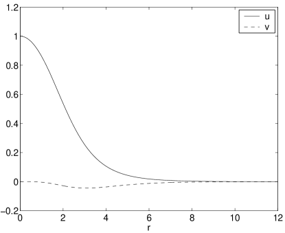
Figure 1: The unique negative eigenmode of the Hessian at the saddle point $\psi_{2}$. The plot shows the radial functions in the parametrisation (3.12) .

4 Unstable manifold and truncated dynamics

The unstable manifold of a saddle point is the union of paths of steepest descent from the saddle point. To define paths of steepest descent, one requires both a metric and a potential. Suppose $x^{i}$ are local coordinates on a finite-dimensional manifold with potential energy $V$ and the metric is represented by the matrix $g_{ij}$. Then the paths of steepest descent are solutions to the gradient flow equations

$$g_{ij}\frac{dx^{j}}{d\tau}=-\frac{\partial V}{\partial x^{i}},$$ (4.1)

with $x^{i}(\tau)$ approaching the relevant saddle point as $\tau\rightarrow-\infty$. It is important to keep track of the metric even when it is flat. For example, gradient flow on $\mathbb{R}^{2}$ with the standard flat metric takes the following form in complex coordinates $z=x_{1}+ix_{2}$:

$$\frac{dz}{d\tau}=-2\frac{\partial V}{\partial\bar{z}}.$$ (4.2)

In the field theory we are considering here the potential energy is the Ginzburg-Landau potential energy functional (1.2) and the metric is the flat metric. Since we work with complex-valued fields, tangent vectors are also complex-valued functions and the metric is the inner product of tangent vectors defined in (3.11). The gradient flow equation is the following non-linear heat equation

$$\partial_{\tau}\psi=-2\frac{\delta E}{\delta\bar{\psi}}=\Delta\psi+(1-|\psi|^{2})\psi.$$ (4.3)

Here $\tau$ is an auxiliary “time” variable, which we distinguish notationally from the time variable $t$ used in the Gross-Pitaevski equation.

We have solved this equation numerically on a grid of size $100\times 100$, corresponding physically to the square $[-20,20]\times[-20,20]$ in the $x_{1}x_{2}$-plane. To generate the gradient flow curve we start with the saddle point configuration $\psi_{2}$ and add a small perturbation $\delta\psi=\epsilon\xi$, where $\xi$ is the negative eigenmode (3.12) found in the previous section. At the boundary of the lattice we impose the Dirichlet boundary condition $\psi(r,\theta)=e^{2i\theta}$. The resulting gradient flow curve does not depend significantly on $\epsilon$ provided it is small enough. When $\epsilon=0$, the discretisation effects provide sufficient perturbation to make sure that the gradient flow curve moves away from the saddle point $\psi_{2}$, but the initial flow is very slow. It is therefore numerically convenient to use a non-vanishing value of $\epsilon$. In figures 2 and 3 we show snapshots of the field and of the energy density during the early stage of the gradient flow, generated by starting with $\delta\psi=0.0005\,\xi$. During the gradient flow, the unstable $n=2$ vortex splits into two $n=1$ vortices which drift apart. The saddle point solution $\psi_{2}$ has an energy density which has a degenerate maximum on a ring. The splitting process begins with the development of two local maxima, as shown in configuration A in figure 3. As the splitting process continues, these local maxima become two distinct vortices. Note, however, that during the early phase of the splitting process, the vortices overlap and deform each other significantly. This is clearly visible in configuration B in figure 3. Only in the later stages of the splitting process do the vortices resemble two standard $n=1$ vortex solutions.

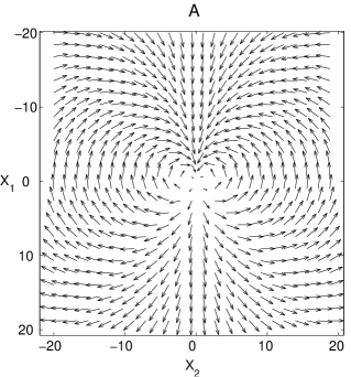
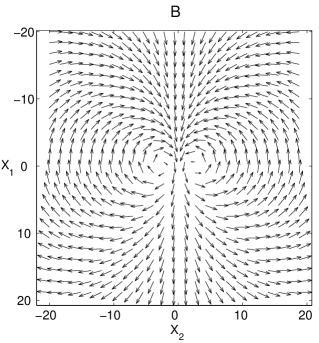
Figure 2: Vortex configurations in the $x_{1}x_{2}$-plane during the early stages of the gradient flow from the saddle point $\psi_{2}$.

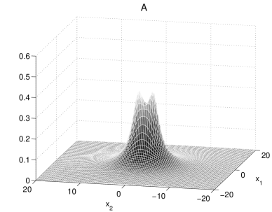
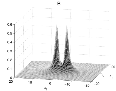
Figure 3: Energy density in the $x_{1}x_{2}$-plane of the vortex configurations A and B of figure 2.

In our numerical simulation of the gradient flow we generated 700 configurations. The most convenient way of labelling these configurations is in terms of their Ginzburg-Landau energy rather than by the configuration number or the gradient flow “time” $\tau$, which have no physical significance in the Gross-Pitaevski model. The finite lattice used in the computation provides a natural renormalisation of the energy of the vortex configurations, assigning the value $E_{\mbox{\tiny ren}}[\psi_{2}]=V_{\mbox{\tiny max}}=31.982$ to the saddle point configuration $\psi_{2}$. The configuration A in figures 2 and 3 has the energy $V=31.955$ and the configuration B has the energy $V=30.257$.

There is another way of parametrising the gradient flow which we need to address, namely the parametrisation in terms of vortex separation. Vortex separation is used as a parameter for pinned vortex configurations in the work of Ovchinnikov and Sigal. In view of our later comparison with that work we therefore make a few comments on it here. The pictures of the vortex configurations and energy densities shown in figures 2 and 3 illustrate that the notion of a separation is not well-defined during the early stages of the gradient flow. The best one can do is to define a functional of vortex configurations which reproduces the distance between the maxima of the energy density (or, equivalently, between the zeros of the field $\psi$) for well-separated vortices and which is computationally convenient. In the following we use the vorticity (2.6) instead of the energy density. The vorticity looks qualitatively very similar to the energy density during all stages of the gradient flow and in particular it is strongly peaked around the zeros of the field $\psi$ for well-separated vortices. The advantage of using the vorticity rather than the energy density is that the total vorticity is conserved whereas the total energy changes during the gradient flow. To motivate our approach further, note that the configurations generated during the gradient flow break the invariance group $R_{2}$ of the saddle point to the group $\mathbb{Z}_{2}\times\mathbb{Z}_{2}$ generated by reflections about the $x_{1}$ and $x_{2}$ axes, each combined with the complex conjugation of $\psi$. As a result the vorticity $\gamma$ of all configurations is reflection symmetric about two orthogonal axes. For our gradient flow the reflection axes are the coordinate axes, and the vortices separate along the $x_{2}$-axis because we have broken the rotational symmetry $R_{2}$ of the saddle point solution explicitly by using the perturbation $\xi$ (3.12). A different perturbation would have led to an isomorphic reflection symmetry about a different set of orthogonal axes, and a different separation direction. We use the reflection axis orthogonal to the separation direction to divide $\mathbb{R}^{2}$ into two half spaces $H_{r}=\{(x_{1},x_{2})\in\mathbb{R}^{2}|x_{2}\geq 0\}$ and $H_{l}=\{(x_{1},x_{2})\in\mathbb{R}^{2}|x_{2}<0\}$. Then we define the separation functional as

$$a[\psi]=\int_{H_{r}}x_{2}\,\gamma\,d^{2}x-\int_{H_{l}}x_{2}\,\gamma\,d^{2}x=2\int_{H_{r}}x_{2}\,\gamma\,d^{2}x.$$ (4.4)

As expected, the separation functional (4.4) increases monotonically during the gradient flow, but one interesting feature is that it assigns a non-vanishing value to the “coincident” vortex configuration $\psi_{2}$. This is a familiar feature of separation parameters used for other solitons, such as monopoles in non-abelian gauge theory [18]. The point is that solitons lose their separate identity when they overlap and separation ceases to be a meaningful concept. In particular there is no reason to insist that a separation parameter vanish for a particular configuration. Numerically, we find the minimal separation to be $a_{\mbox{\tiny min}}=a[\psi_{2}]=4.815$, which corresponds roughly to the diameter of the ring on which the energy density of $\psi_{2}$ is maximal. For the configuration A in figures 2 and 3 we find $a=4.896$ and for configuration B we find $a=6.406$. The lowest energy configuration we generated has the energy $V=24.405$ and separation $a=15.570$.

For the construction of the unstable manifold we return to the parametrisation of the gradient flow curve in terms of renormalised energy. Thus we obtain a family of fields $\hat{\Psi}(V;x)$, labelled by the value $V$ of the renormalised Ginzburg-Landau energy. According to the general prescription of [10] we should now act with the full symmetry group (2.17) to generate a family of saddle points and a family of gradient flow curves, and use their union as the collective coordinate manifold for the truncated dynamics. However, we are only interested in the relative motion of the two vortices in the fission process and not in their centre-of-mass motion. The latter can be found by applying Galilean boosts (2.18) to the entire configuration. Furthermore, we exclude collective coordinates which change our boundary condition. Both phase rotations and spatial rotations change the field “at infinity” (or at the boundary of our lattice), but the subgroup $R_{2}$ defined in (3.1) respects the boundary condition. It also leaves the saddle point solution $\psi_{2}$ invariant but it acts non-trivially on the gradient curve emanating from $\psi_{2}$. Thus we obtain a family of fields

$$\Psi(V,\chi;r,\theta)=\hat{\Psi}(V;r,\theta-\chi)e^{2i\chi}$$ (4.5)

depending on two collective coordinates $V,\chi$. The former measures the energy and the second labels the spatial orientation of the two-vortex configurations generated during the gradient flow. Since the saddle point configuration with energy $V_{\mbox{\tiny max}}$ does not depend on the angle $\chi$, the collective coordinate manifold is topologically a plane, with $(V_{\mbox{\tiny max}}-V,\chi)$ as polar coordinates. We denote this manifold by ${\cal M}_{2}$. The range of the angle $\chi$ is $[0,\pi)$ since the configurations $\hat{\Psi}(V;x)$ generated during the gradient flow are invariant under a rotation by $\pi$ (which is the product of the reflections at the coordinate axes discussed above). Note that ${\cal M}_{2}\subset{\cal C}_{2}$.

It is now a simple matter to compute the restriction of the Gross-Pitaevski Lagrangian (2.1) to ${\cal M}_{2}$. We allow the collective coordinates $V$ and $\chi$ to depend on time and insert the fields $\Psi(V(t),\chi(t);r,\theta)$ into (2.1). The result is

$$L[\Psi(V,\chi;\cdot)]=-\frac{1}{2}\bigl{(}2Q(V)-J(V)\bigr{)}\dot{\chi}-\frac{1}{2}G(V)\dot{V}-V,$$ (4.6)

where we have written $Q(V)$ and $J(V)$ for the Noether charges (2.19) and (2.20) evaluated on $\Psi(V,\chi;x)$, i.e.

$$Q(V)=\int|\Psi(V,\chi;x)|^{2}\,d^{2}x$$ (4.7)

and

$$J(V)=\int\mbox{Im}\left(\bar{\Psi}(V,\chi;x)\frac{\partial\Psi}{\partial\theta}(V,\chi;x)\right)\,d^{2}x.$$ (4.8)

The integrals defining $Q$ and $V$ are both divergent, but the combination

$$K(V)=J(V)-2Q(V)$$ (4.9)

occuring in the Lagrangian is finite. To see this note that for the saddle point configuration $\psi_{2}$ one computes $J=2Q$, so that $K(V_{\mbox{\tiny max}})=0$. As the configuration evolves away from the saddle point $K$ grows but it remains finite for any finite value of $V$. This follows from the continuity of the semigroup defined by the evolution equation 4.3 in a suitable norm, see [14] and [15], and from the continuity of the funtionals $J$ and $Q$ (2.19) and (2.20) with respect to that norm. Finally, the function $G(V)$ is

$$G(V)=\int\mbox{Im}\left(\bar{\Psi}(V,\chi;x)\frac{\partial\Psi}{\partial V}(V,\chi;x)\right)\,d^{2}x.$$ (4.10)

Neither $K$ nor $G$ depends on $\chi$ because of the rotationally invariant integration measure and because the integrands are independent of the phase of $\Psi$. The term $G(V)\dot{V}$ is a total time derivative which does not affect the equations of motion. We therefore omit it in our final expression for the induced Lagrangian $L_{2}$ on ${\cal M}_{2}$:

$$L_{2}=\frac{1}{2}K(V)\dot{\chi}-V.$$ (4.11)

The Euler-Lagrange equations are very simple because our truncated system, like the original Gross-Pitaevski dynamics, is rotationally invariant and has a conserved energy. Thus $V$ remains constant during the time evolution, and the angle $\chi$ changes according to

$$\dot{\chi}(V)=\frac{2}{K^{\prime}(V)}.$$ (4.12)

It follows from the constancy of $V$ that $\dot{\chi}$ is also constant during the time evolution. We introduce the abbreviation

$$\omega(V)=\dot{\chi}(V)$$ (4.13)

for the rate of change of the angle $\chi$. The dependence of this angular velocity on $V$ is the main dynamical information we extract from our truncated dynamics. It is is given by the differential quotient

$$\omega(V)=2\frac{dV}{dK}.$$ (4.14)

Numerically, we compute $\omega$ by evaluating finite difference quotients $\Delta V/\Delta K$ of successive configurations. Our results are displayed in figure 4. In the early phase of the gradient flow (roughly the first 100 configurations) both $V$ and $K$ change very slowly and accurate numerical computation of the difference quotient is difficult. We have omitted these difference quotients from our plot. Since the energy $V$ hardly changes during this part of the gradient flow, this omission makes no visible to difference to the graph $\omega(V)$ shown in figure 4. The next section is devoted to a detailed discussion and interpretation of our results.

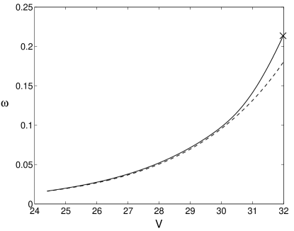
Figure 4: The solid line shows the angular velocity $\omega$ of two-vortex configurations as a function of the energy $V$. The dependence of $\omega$ on the energy predicted by the Kirchhoff-Onsager law is plotted with a dashed line. The value of $\omega_{\mbox{\tiny max}}$ given in (5.9) is marked with a “$\times$”.

5 Orbiting vortex pairs

Our two-dimensional Lagrangian dynamical system $({\cal M}_{2},L_{2})$ is designed to approximate the slow interactive dynamics of two vortices moving according to the Gross-Pitaevski equation (1.13). The model predicts that the two vortices will orbit each other, with the angular frequency depending on their total energy as shown in our figure 4. While the qualitative behaviour of the two vortex system is not surprising and familiar from vortices in ordinary fluids and also vortices in the gauged Ginzburg-Landau model [16], the precise prediction of the variation of the angular frequency with the energy for both overlapping and well-separated vortices is new. In [13] Dziarmaga computed the rotation frequency of an overlapping vortex pair by linearising the Gross-Pitaevski equation around the saddle point solution $\psi$. The linearised solution is

$$\psi(t,x)=\psi_{2}(x)+\epsilon e^{-i\lambda t}(u(r)+e^{4i\theta}v(r)),$$ (5.1)

where $\lambda$ and $(u,v)$ are the eigenvalue and eigenfunctions of the eigenvalue problem (3). The interpretation of the linearised solution in terms of rotating vortices requires some care. As we saw in section 3, the radial eigenfunction $v$ is much smaller than $u$. Thus, as a first approximation, we may think of (5.1) as a field whose magnitude depends on $r$ according to $\epsilon u(r)$ and whose direction changes with angular frequency $\lambda$, all superimposed on the static $n=2$ solution. The effect of such a superposition is a configuration with two zeros (whose separation depends on $\epsilon$) which rotate around one another with angular velocity $\omega_{\mbox{\tiny lin}}=-\lambda/2$. The factor $1/2$ arises because for $\psi_{2}$ a phase rotation by $\alpha$ is equivalent to a spatial rotation by $\alpha/2$. With our value for $\lambda$, we thus find $\omega_{\mbox{\tiny lin}}=-\lambda/2=0.20935$.

In the limit $V\rightarrow V_{\mbox{\tiny max}}$ our numerically computed function $\omega(V)$ approaches a value which is close to but not exactly equal to $\omega_{\mbox{\tiny lin}}$. The discrepancy arises because we neglected the radial eigenfunction $v$ in our interpretation of the linearised solution. We can establish a precise relation between the eigenvalue $\lambda$ and the limiting angular frequency

$$\omega_{\mbox{\tiny max}}:=\lim_{V\rightarrow V_{\mbox{\tiny max}}}\omega(V)$$ (5.2)

as follows. Using the definition (4.9) and noting that both $V$ and $K$ are originally defined along the gradient flow curve parametrised in terms of the auxiliary variable $\tau$ (4.3) we write

$$\omega(V)=2\frac{dV}{dK}=2\frac{dV}{d\tau}/\frac{dK}{d\tau}.$$ (5.3)

Recall that we computed our gradient flow curve by starting at $\tau=0$ with the configuration $\psi_{2}+\epsilon\xi$, where $\xi$ is the eigenmode (3.12) and $\epsilon$ is small (in practice $\epsilon=0.0005$). At that point the gradient of the Ginzburg-Landau energy functional is

$$\frac{\delta E}{\delta\bar{\psi}}[\psi_{2}+\epsilon\xi] \approx \epsilon\frac{\delta^{2}E}{\delta\psi\delta\bar{\psi}}\xi+\epsilon\frac{\delta^{2}E}{\delta\bar{\psi}^{2}}\bar{\xi}$$ (5.4)

$$= \frac{1}{2}\lambda\epsilon\xi,$$

where we have used that the first functional derivative of $E$ vanishes at $\psi_{2}$ and that $\xi$ is an eigenfunction of the Hessian, i.e. it satisfies (3.8). Hence from (4.3)

$$\partial_{\tau}\psi_{|_{\tau=0}}\approx-\lambda\epsilon\xi\quad\mbox{and}\quad\partial_{\tau}\bar{\psi}_{|_{\tau=0}}\approx-\lambda\epsilon\bar{\xi}$$ (5.5)

and thus

$$\left.\frac{dV}{d\tau}\right|_{\tau=0} = \int\frac{\delta E}{\delta\psi}[\psi_{2}+\epsilon\xi]\,\,\partial_{\tau}\psi_{|_{\tau=0}}+\frac{\delta E}{\delta\bar{\psi}}[\psi_{2}+\epsilon\xi]\,\,\partial_{\tau}\bar{\psi}_{|_{\tau=0}}\,d^{2}x$$ (5.6)

$$\approx -\epsilon^{2}\lambda^{2}\int\bar{\xi}\xi\,d^{2}x$$

$$= -\epsilon^{2}\lambda^{2}\cdot 2\pi\int(u^{2}+v^{2})\,rdr,$$

where we used (5.5) and inserted the expression (3.12) for $\xi$.

It is easy to check that any $R_{2}$-invariant configuration (3.1) and hence in particular $\psi_{2}$ is a stationary point of the functional $K[\psi]$ (4.9). Thus $\frac{\delta K}{\delta\psi}(\psi_{2})=0$ and by a similar calculation to the one given above we have

$$\left.\frac{dK}{d\tau}\right|_{\tau=0} = \int\frac{\delta K}{\delta\psi}[\psi_{2}+\epsilon\xi]\,\,\partial_{\tau}\psi_{|_{\tau=0}}+\frac{\delta K}{\delta\bar{\psi}}[\psi_{2}+\epsilon\xi]\,\,\partial_{\tau}\bar{\psi}_{|_{\tau=0}}\,d^{2}x$$ (5.7)

$$\approx -\epsilon^{2}\lambda\int\bar{\xi}\frac{\delta^{2}K}{\delta\bar{\psi}\delta\psi}\xi+\xi\frac{\delta^{2}K}{\delta\psi\delta\bar{\psi}}\bar{\xi}$$

$$= -2\epsilon^{2}\lambda\int\left(\mbox{Im}\bar{\xi}\partial_{\theta}\xi-2\xi\bar{\xi}\right)\,d^{2}x$$

$$= 4\epsilon^{2}\lambda\cdot 2\pi\int(u^{2}-v^{2})\,rdr,$$

where we used that $\delta^{2}K/\delta\psi^{2}=\delta^{2}K/\delta\bar{\psi}^{2}=0$. The approximate equalities become exact in the limit $\epsilon\rightarrow 0$. Thus we find the following exact expression for the angular frequency $\omega_{\mbox{\tiny max}}$ (5.2) in terms of the eigenvalue $\lambda$:

$$\omega_{\mbox{\tiny max}}=-\frac{\lambda}{2}\frac{\int\,(u^{2}+v^{2})rdr}{\int\,(u^{2}-v^{2})rdr}.$$ (5.8)

In view of the numerical difficulties in computing $\omega$ near the saddle point this formula is very useful in practice. Evaluating it numerically we find

$$\omega_{\mbox{\tiny max}}=-\frac{\lambda}{2}\times 1.0200=0.21354.$$ (5.9)

This value provides a check on our computation of $\omega(V)$ near the saddle point and is marked with a “$\times$” in figures 4 and 5.

For well-separated vortices we can compare our results with those obtained by Neu in [3, 4] via scaling techniques or those obtained by Ovchinnikov and Sigal in [8] based on pinned vortex configurations. Both find that well-separated vortices are governed by the Kirchhoff-Onsager law. According to that law two vortices separated by a distance $a$ have an interaction energy given by

$$V(a)=-2\pi\ln a+C,$$ (5.10)

where $C$ is an arbitrary normalisation constant, and orbit each other with angular frequency

$$\omega_{\mbox{\tiny KO}}=\frac{4}{a^{2}}.$$ (5.11)

It follows that the rotation frequency is given as a function of the energy via

$$\omega_{\mbox{\tiny KO}}(V)=\tilde{C}e^{\frac{V}{\pi}},$$ (5.12)

where $\tilde{C}=4\exp(-C/\pi)$. The constant $C$ (and hence $\tilde{C}$) is determined once the dependence of the energy on the vortex separation is known. To make contact with the Kirchhoff-Onsager relations we thus have to make use of the separation functional introduced for our vortex configurations in (4.4). We pick a vortex configuration consisting of clearly separated vortices and compute its energy to be $V=27.253$ and its separation to be $a=10.012$. Inserting these values into (5.10) fixes the value of $C$ and hence $\tilde{C}$. We have plotted the resulting function (5.12) in figure 4. It is important to be clear about the interpretation of the two curves in figure 4. For well-separated vortices we can meaningfully associate a separation parameter to a vortex configuration. The Kirchhoff-Onsager relation gives the angular frequency of point-vortices with that separation. The fact that for low energy configurations consisting of well-separated vortices the Kirchhoff-Onsager relation agrees with our results shows that well-separated vortices may be treated as point-vortices, in agreement with the results of Ovchinnikov and Sigal in [8]. The two curves in figure 5 differ for configurations near the saddle point, not so much because the predictions of our model disagree with those of the point vortex model but because the two models are no longer compatible in that regime.

From the point of view of the Kirchhoff-Onsager relation, the dependence (5.11) of the angular velocity on separation is more fundamental than the dependence on the energy. In figure 5 we plot the angular velocity $\omega$ as a function of the separation parameter (4.4) and compare it with the simple Kirchhoff-Onsager prediction. Again the two plots agree for large separations, and the comments made above on the comparison near the saddle point apply here, too. However, it is worth emphasising that the Kirchhoff-Onsager relation predicts a divergence of the angular velocity when the separation tends to zero. Our results show that for the Ginzburg-Landau vortices this divergence is removed, essentially by cutting off small separation parameters. This is yet another example of a soliton model “regularising” the singularities of a point-particle model.

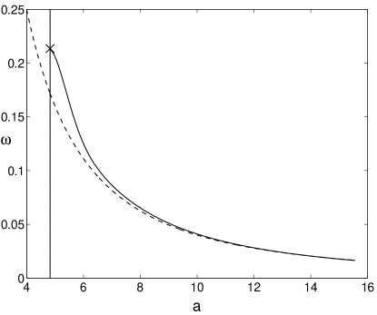
Figure 5: The solid line shows the angular velocity $\omega$ of two-vortex configurations as a function of the separation $a$. The dependence of $\omega$ on the separation predicted by the Kirchhoff-Onsager law is plotted with a dashed line. The value of $\omega_{\mbox{\tiny max}}$ given in (5.9) is marked with a “$\times$”.

6 Discussion and Conclusion

The unstable manifold method used in this paper to approximate the dynamics of interacting vortices in the Gross-Pitaevski model allows one to analyse the relative motion of two vortices at arbitrary separation. When the vortices are overlapping our results reproduce those found with linearisation methods and when the vortices are well-separated our results agree with the Kirchhoff-Onsager law. Our method gives a unified description of both regimes, and successfully interpolates between them.

When vortices evolve according to the Gross-Pitaevski equation they will in general also emit radiation. This effect is not captured in our approximation. However, it is possible to compute radiative corrections to the vortex motion predicted by our approximation using the methods developed by Ovchinnikov and Sigal in [9]. In particular, Ovchinnikov and Sigal studied the radiative corrections to the orbiting motion of a vortex pair and found that, for large vortex separation $a$, the power emitted in the radiation is proportional to $a^{-6}$. As a result of this energy loss, the orbiting vortices drift apart slowly as they orbit each other. However, since the power loss is small, the change of the separation during one period of rotation is also small (much less than 1 %). Combining these results with our calculations, we arrive at the following qualitative picture of vortex fission in the Gross-Pitaevski model. Suppose the $n=2$ saddle point solution is perturbed and allowed to evolve according to the Gross-Pitaevski equation. The perturbed vortex configuration rotates and emits radiation. The radiation carries away energy and the vortex configuration adjusts by finding a configuration of lower energy. The most efficient way of doing so is by following a path of steepest (energy) descent. As we have seen, the $n=2$ vortex breaks up into two $n=1$ vortices along the path of steepest descent. Thus we can use our truncated dynamical system $({\cal M}_{2},L_{2})$ and expect the vortex pair to orbit with the angular frequency depending on the energy according to (4.12). The continued rotation results in further emission of radiation and loss of energy, to which the vortex pair adjusts by drifting further apart. The fission process is thus governed by the combination of two effects: the radiation carries away energy and the vortex configuration adjusts by sliding down the unstable manifold of the $n=2$ saddle point. It would be interesting to make this picture more precise by studying the radiation effects quantitatively. This should probably be done in conjunction with a more careful study of the conservation laws in the theory, similar to the investigation for gauged vortices in [17]. As mentioned briefly in section 2, the conservation of angular momentum can also be expressed as the conservation of the moment (2.22) of the vorticity. Just looking at vortex motion during the fission process it seems that the moment (2.22) increases as the vortices drift apart. It would be interesting to understand how the radiation makes up for this change, possibly by carrying negative vorticity off to infinity.

We would like to emphasise that the work described here is the first application of the unstable manifold method to soliton dynamics in more than one spatial dimension. As such, it contains a number of useful general lessons. At first sight it may not seem sensible to use one non-linear partial differential equation (the gradient flow equation) to approximate another non-linear partial differential equation (the Gross-Pitaevski equation). However, generally speaking, gradient flow is easier to understand and to compute numerically than Hamiltonian flow like that defined by the energy-conserving Gross-Pitaevski equation. One reason for this is that the typical time scales of the two evolution processes are very different. Our discussion of the vortex fission process illustrates this point. The solution of the gradient flow equation over a relatively short CPU time (roughly 700 steps) maps out all the interesting configurations between the $n=2$ saddle point and the well-separated vortices. The fission process according to the Gross-Pitaevski equation, by contrast, is expected to take several orders of magnitude longer, making it difficult to maintain numerical accuracy. The gradient flow equation provides an efficient way of mapping out those configurations which are relevant for slow (or low-energy) dynamics. At a more practical level, we found that the explicit study of the linear negative modes of the saddle point was essential for an efficient computation of the unstable manifold. We expect that this will become even more important for saddle points with more than one negative mode. Thus one could repeat the calculations performed here for the saddle point solutions $\psi_{n}$ with vortex number $n>2$. As explained in [2], there is now more than one unstable mode. As a first step in constructing the unstable manifold of these saddle points one needs to compute the negative eigenmodes of the linearised Ginzburg-Landau equation explicitly. While the explicit construction of the unstable manifolds and the computation of the induced dynamics may be difficult, it would be interesting to understand general geometrical features of the unstable manifolds and use them to derive qualitative features of multi-vortex dynamics in the Gross-Pitaevski model.

It remains an open problem to justify the unstable manifold approximation used in this paper analytically. The fact that our results agree with those obtained via more familiar approximations in limiting regimes provides an encouraging check. However, this agreement also raises a question. Near the saddle point our method agrees with results obtained by linearisation, and the small parameter controlling the validity of the approximation is the amplitude $\epsilon$ in (5.1). As explained, this is related to the separation of the two zeros of the field $\psi$. Far away from the saddle point, our approximation agrees with the point-vortex model implicit in the Kirchhoff-Onsager law. The small parameter controlling the validity of the approximation in this regime is the inverse separation of the zeros of $\psi$ (i.e. the inverse distance between the vortices). Since our method interpolates between the two approximations it is not clear which, if any, small parameter controls the approximation in the intermediate regime. More generally, proof of the validity of the approximation, possibly along the lines of the proof of the geodesic approximation for gauged vortex dynamics in [19], would be very desirable. A useful starting point for such an investigation may be the following natural relation between the gradient flow equation (4.3) and the Gross-Pitaevski equation (1.13). Both define flows in the space ${\cal C}$ (2.4) in terms of the Ginzburg-Landau energy. However, the gradient flow uses the inner product (3.11) whereas the Gross-Pitaevski equation is a Hamiltonian flow using the symplectic structure (2.9). The inner product (3.11) and the symplectic form (2.9) are equal to, respectively, the real and imaginary part of the sesquilinear form

$$g(\vec{\xi},\vec{\eta})=\int_{\mathbb{R}^{2}}\xi\bar{\eta}\,\,d^{2}x.$$ (6.1)

One interesting manifestation of this relationship is that gradient flow trajectories and solutions of the Gross-Pitaevski equation are orthogonal with respect to the inner product (3.11) whenever they intersect.

Acknowledgements

Most of the research reported here was carried out while OL was an MSc student at Heriot-Watt University. OL thanks the DAAD for a scholarship during that time and Dugald Duncan for advice on the numerical calculations. BJS acknowledges an EPSRC advanced research fellowship.

References

- [1] Bethuel F, Brézis H and Hélein F 1994 Ginzburg-Landau vortices (Basel: Birkhäuser)
- [2] Ovchinnikov Y N and Sigal I M 1997 Ginzburg-Landau equation I. Static vortices, in Partial differential equations and their applications CRM Proceedings and Lecture Notes 12 199–220, eds Greiner P et al (Providence: American Mathematical Society)
- [3] Neu J C 1990 Vortices in complex scalar fields, Physica D 43 385–406
- [4] Neu J C 1990 Vortex dynamics of the non-linear wave equation Physica D 43 407–420
- [5] Lin F-H and Xin J X 1999 On the imcompressible fluid limit and the vortex motion law of the nonlinear Schrödinger equation Commun. Math. Phys. 200 249–274
- [6] Lin F-H and Xin J X 1999 On the dynamical law of the Ginzburg-Landau vortices on the plane Comm. Pure Appl. Math. 52 1189–1212
- [7] Colliander J E and Jerrard R L 1998 Vortex dynamics for the Ginzburg-Landau-Schrödinger equation Internat. Math. Res. Notices 7 333–358
- [8] Ovchinnikov Y N and Sigal I M 1998 The Ginzburg-Landau equation III. Vortex dynamics Nonlinearity 11 1277–1294
- [9] Ovchinnikov Y N and Sigal I M 1998 Long-time behaviour of Ginzburg-Landau vortices Nonlinearity 11 1275–1310
- [10] Manton N S 1988 Unstable manifolds and soliton dynamics Phys. Rev. Lett. 60 1916–1919
- [11] Manton N S and Merabet H 1997 kinks – gradient flow and dynamics Nonlinearity 10 3–18
- [12] Papanicolaou N and Tomaras T N 1993 On the dynamics of vortices in a nonrelativistic Ginzburg-Landau model Phys. Lett. A 179 33
- [13] Dziarmaga J 1996 Dynamics of overlapping vortices in complex scalar fields Act. Phys. Pol. B27 1943–1960
- [14] Ginibre J and Velo G 1996 The Cauchy problem in local spaces for the complex Ginzburg-Landau equation I. Compactness methods Physica D 95 191–228
- [15] Ginibre J and Velo G 1997 The Cauchy problem in local spaces for the complex Ginzburg-Landau equation II. Contraction methods Commun. Math. Phys. 187 45–79
- [16] Manton N S 1997 First order vortex dynamics Annals Phys. 256 114–131
- [17] Manton N S and Nasir S M 1999 Conservation laws in a first order dynamical system of vortices Nonlinearity 12 851–865
- [18] Atiyah M and Hitchin N 1988 Geometry and dynamics of monopoles (Princeton: Princeton University Press)
- [19] Stuart D 1994 Dynamics of abelian Higgs vortices in the near Bogomolny regime Commun. Math. Phys. 159 51–91.