Lyapunov Spectra of Periodic Orbits for a Many-Particle System

The Lyapunov spectrum corresponding to a periodic orbit for a two dimensional many particle system with hard core interactions is discussed. Noting that the matrix to describe the tangent space dynamics has the block cyclic structure, the calculation of the Lyapunov spectrum is attributed to the eigenvalue problem of $16\times 16$ reduced matrices regardless of the number of particles. We show that there is the thermodynamic limit of the Lyapunov spectrum in this periodic orbit. The Lyapunov spectrum has a step structure, which is explained by using symmetries of the reduced matrices.

1 Introduction

Just as low dimensional chaos is revealed by a single positive Lyapunov exponent which indicates exponential sensitivity to initial conditions, systems with phase space of very high dimension can be characterized by their Lyapunov spectra which give information about many possible instabilities in the system. As a concrete example, we consider the system consisting of $N$ disks with hard core interactions and periodic boundary conditions. This is a surprisingly good model of a fluid [1], and yet is sufficiently simple that ergodic properties may be established under fairly general conditions [2].

The following is a brief review of the study of Lyapunov spectra in such systems; for more details and references in numerical work, see Ref. [3] and in analytical work, see Ref. [4]. It has been known for some time that the Lyapunov exponents of Hamiltonian systems come in plus/minus pairs, that is, the spectrum is symmetric about zero [5]. Non-equilibrium extensions were shown to exhibit symmetry about a point other than zero [6, 7], leading to the discovery that these extensions also contain hidden Hamiltonian structure [8, 9]. Also known for more than twenty years is the algorithm for numerical computation of Lyapunov exponents due to Benettin and others [10, 11]. Later, a constraint method was introduced [12]. More recently, the effects of the hard collisions have been properly taken into account [3, 13]. The existence of a thermodynamic limit in Lyapunov spectra, that is, that the spectrum retains its shape as the number of particles increases, has been put forward using random matrix approximations [14], numerical evidence [15] and mathematical arguments [16], but recent numerical work has suggested in contrast, a logarithmic singularity of the largest Lyapunov exponent with the number of particles [17]. Lyapunov spectra for diatomic molecules (represented by dumb-bells) show an explicit separation of the rotational and translational degrees of freedom if the departure from sphericity is small enough [18]. Finally, and of particular interest to us, careful simulations of sufficiently large systems have revealed a step structure in the Lyapunov spectrum for the smallest positive Lyapunov exponents [3, 13, 18]. The above references give an incomplete description in terms of “Posch Lyapunov modes”, phase space perturbations corresponding to these small Lyapunov exponents which are approximately sinusoidal in position space. Recently Eckmann and Gat have suggested an explanation of the Lyapunov modes of a one dimensional system using a random matrix approximation of the Lyapunov spectrum [19]. In this paper we study step structure in the Lyapunov spectrum of a two dimensional many particle system without making any approximations, however we are restricted to periodic orbits.

Periodic orbit theory [20, 21] has proven very useful for investigations of the corresponding low dimensional system, the periodic Lorentz gas [22, 23, 24, 25], computing properties such as the diffusion coefficient. These methods cannot generally be applied directly to high dimensional systems due to the difficulty of finding all the periodic orbits, although a notable exception is the Kuramoto-Shivashinsky PDE in a regime where the effective number of degrees of freedom is small [26]. However, periodic orbit arguments have been used to justify thermodynamic results such as non-negativity of the entropy production [27] and the Onsager relations [28] without explicitly finding any periodic orbits. Periodic orbits of spatially extended systems in the form of coupled map lattices have been considered previously [29, 30], leading to block cyclic matrices similar to those observed in this paper.

Here we apply methods similar to those to Ref.[30] to reduce the problem of computing the Lyapunov spectrum to that of finding the eigenvalues of a relatively small ($16\times 16$) matrix. A step structure is observed, which is related to the symmetries of the system. Our formalism shows that, at least in the case of this periodic orbit, the thermodynamic limit of the Lyapunov spectrum holds exactly.

2 Lyapunov Exponents of Periodic Orbits for the Many-Particle System

The system which we consider in this paper is a two-dimensional Hamiltonian system consisting of $N$ disks, interacting only by hard core collisions. We choose units such that the mass and radius of the particles are one. We write the position and the momentum of the $j$-th particle as $\mbox{\boldmath$\it q$}_{j}$ and $\mbox{\boldmath$\it p$}_{j}$, respectively, and for a later convenience we represent the phase space vector $\it\Gamma$ as a column vector $(\mbox{\boldmath$\it q$}_{1},\mbox{\boldmath$\it p$}_{1},\mbox{\boldmath$\it q$}_{2},\mbox{\boldmath$\it p$}_{2},\cdots,\mbox{\boldmath$\it q$}_{N},\mbox{\boldmath$\it p$}_{N})^{T}$ with $T$ the transpose operation.

The dynamics of such a many-particle system is simply separated into the free flight part and the collision part, and the tangent vector $\delta\mbox{\boldmath$\it\Gamma$}_{n}$ of the phase space just after the $n$-th collision occurs is related to the tangent vector $\delta\mbox{\boldmath$\it\Gamma$}_{0}$ at the initial time by $\delta\mbox{\boldmath$\it\Gamma$}_{n}=M_{n}\delta\mbox{\boldmath$\it\Gamma$}_{0}$ with the $4N\times 4N$ matrix $M_{n}$ represented as

$$M_{n}\equiv M_{n}^{(c)}M_{n}^{(f)}M_{n-1}^{(c)}M_{n-1}^{(f)}\cdots M_{1}^{(c)}M_{1}^{(f)}.$$ (1)

Here $M_{j}^{(f)}$ is the $4N\times 4N$ matrix to specify the $j$-th free flight dynamics, and is given by

$$M_{j}^{(f)}\equiv\mbox{Diag}(L_{1}^{(1)},L_{2}^{(1)},\cdots,L_{N}^{(1)})$$ (2)

where $\mbox{Diag}(X_{1},X_{2},\cdots,X_{l})$ means the matrix on whose diagonal are the matrix blocks $X_{1},X_{2},\cdots,X_{l}$ for an integer $l$, and $L_{j}^{(1)}$ is defined by

$$L_{j}^{(1)}\equiv\left(\begin{array}[]{cc}\underline{I}&\tau_{j}\underline{I}\\ \underline{0}&\underline{I}\end{array}\right)$$ (5)

where $\underline{I}$ and $\underline{0}$ are $2\times 2$ identical and null matrices, respectively, and $\tau_{j}$ is its corresponding free flight time. On the other hand, $M_{j}^{(c)}$ is the $4N\times 4N$ matrix to specify the $j$-th collision of particles. For the simplest case in which the $j$-th collision involves only the $k_{j}$-th and the $l_{j}$-th particles colliding, the matrix $M_{j}^{(c)}$ is given as the block matrix

$$M_{j}^{(c)}\equiv\left(\begin{array}[]{cccccccc}\tilde{I}&&&&&&&\\ &&\ddots&&&&&\\ &&&F_{j}&&G_{j}&&\\ &&&&\ddots&&&\\ &&&G_{j}&&F_{j}&&\\ &&&&&&\ddots&\\ &&&&&&&\tilde{I}\end{array}\right)\begin{array}[]{cccccccc}\\ \leftarrow\;\;\;k_{j}\\ \\ \\ \leftarrow\;\;\;l_{j}\\ \\ \end{array}$$ (19)

$$\begin{array}[]{cccccccc}&&\uparrow&&&&\uparrow&\\ &&k_{j}&&&&l_{j}&\end{array}\begin{array}[]{cccccccc}\\ \\ \\ \\ \\ \\ \end{array}$$ (28)

where $\tilde{I}$ is the $4\times 4$ identity matrix and is put in the part of $\ddots$ of the above representation, and $F_{j}$ ($G_{j}$) is the $(k_{j},k_{j})$ and $(l_{j},l_{j})$ ($(k_{j},l_{j})$ and $(l_{j},k_{j})$) block matrix elements, and the $4\times 4$ null matrices are put in the other elements. Here $4\times 4$ matrices $F_{j}$ and $G_{j}$ are defined by [13]

$$F_{j}\equiv\left(\begin{array}[]{cc}\underline{I}-L_{j}^{(2)}&\underline{0}\\ -L_{j}^{(3)}&\underline{I}-L_{j}^{(2)}\end{array}\right)$$ (31)

$$G_{j}\equiv\left(\begin{array}[]{cc}L_{j}^{(2)}&\underline{0}\\ L_{j}^{(3)}&L_{j}^{(2)}\end{array}\right)$$ (34)

with the $2\times 2$ matrices $L_{j}^{(2)}$ and $L_{j}^{(3)}$ defined by

$$L_{j}^{(2)}\equiv\mbox{\boldmath$\it n$}_{j}\mbox{\boldmath$\it n$}_{j}^{T}$$ (35)

$$L_{j}^{(3)}\equiv\mbox{\boldmath$\it n$}_{j}^{T}\Delta\mbox{\boldmath$\it p$}^{(j)}\left(\underline{I}+\frac{\mbox{\boldmath$\it n$}_{j}\Delta\mbox{\boldmath$\it p$}^{(j)T}}{\mbox{\boldmath$\it n$}_{j}^{T}\Delta\mbox{\boldmath$\it p$}^{(j)}}\right)\left(\underline{I}-\frac{\Delta\mbox{\boldmath$\it p$}^{(j)}\mbox{\boldmath$\it n$}^{T}}{\Delta\mbox{\boldmath$\it p$}^{(j)T}\mbox{\boldmath$\it n$}_{j}}\right),$$ (36)

(Note that all vectors in this paper are introduced as column vectors, so for example, $\mbox{\boldmath$\it n$}_{j}^{T}\Delta\mbox{\boldmath$\it p$}^{(j)}$ is a scalar and $\mbox{\boldmath$\it n$}_{j}\Delta\mbox{\boldmath$\it p$}^{(j)T}$ is a matrix.) where $\mbox{\boldmath$\it n$}_{j}$ is the unit vector pointing from the center of the $k_{j}$-th disk to the center of the $l_{j}$-th disk at the $j$-th collision, and $\Delta\mbox{\boldmath$\it p$}^{(j)}$ is the momentum difference $\mbox{\boldmath$\it p$}_{l_{j}}-\mbox{\boldmath$\it p$}_{k_{j}}$ just before the $j$-th collision.

Now we consider the case that the movement of the system is periodic in time, so that the condition $\mbox{\boldmath$\it\Gamma$}_{n_{p}}=\mbox{\boldmath$\it\Gamma$}_{0}$ is satisfied for a integer $n_{p}$. In this case the Lyapunov exponents $\lambda_{j}$, $j=1,2,\cdots,4N$ of the periodic orbit are defined by $\lambda_{j}=(1/t(n_{p}))\ln|m_{j}(n_{p})|$ in terms of the absolute value of the (generally complex) eigenvalue $m_{j}(n_{p})$ of the matrix $M_{n_{p}}$, where $t(n_{p})\equiv\sum_{j=1}^{n_{p}}\tau_{j}$ is the period of this orbit.

We put the set of the Lyapunov exponents in descending order, namely $\lambda_{1}\geq\lambda_{2}\geq\cdots\geq\lambda_{4N}$. It is well known that in the time-independent Hamiltonian system the Lyapunov exponents satisfy the pairing rule [5], namely the condition $\lambda_{1}+\lambda_{4N}=\lambda_{2}+\lambda_{4N-1}=\cdots=\lambda_{2N}+\lambda_{2N+1}=0$. Noting this fact, thereafter we consider only the first half $\lambda_{1}$, $\lambda_{2},\cdots,\lambda_{2N}$ of the full Lyapunov exponents, and refer their set as the Lyapunov spectrum in this paper.

3 Periodic Orbit Model and the Reduced Matrix

By using the method given in the previous section, we calculate the Lyapunov spectrum for the periodic orbit illustrated in Fig. 1. In this periodic orbit each particle moves in a square orbit with the same absolute value of momentum and the same direction of rotation and with a constant free flight time $\tau$ (So the period of the orbit is $t(4)=4\tau$.). We put $2N_{1}$ ($2N_{2}$) as the number of the particles in each horizontal line (each vertical line) so that $N=4N_{1}N_{2}$. We impose periodic boundary conditions, thus requiring the number of particles in each direction to be even.

Figure 1: Periodic orbit of the many particle system. The circular dots show the positions of particles at the initial time, and the solid lines give the subsequent path in the direction of the arrows.

In this periodic orbit model, there are only two types of collisions illustrated in Fig. 2, in which the trajectories of two colliding particles are drawn with their moving directions shown by the arrows. Now we consider the dynamics of particles for a free flight plus one of these two collisions. Such a dynamics is described by the matrix multiplications $\tilde{F}_{1}\equiv F_{1}\mbox{Diag}(L_{1}^{(1)},L_{1}^{(1)})$ and $\tilde{G}_{1}\equiv G_{1}\mbox{Diag}(L_{1}^{(1)},L_{1}^{(1)})$ ($\tilde{F}_{2}\equiv F_{2}\mbox{Diag}(L_{2}^{(1)},L_{2}^{(1)})$ and $\tilde{G}_{2}\equiv G_{2}\mbox{Diag}(L_{2}^{(1)},L_{2}^{(1)})$) corresponding to the left (right) orbit in Fig. 2. By using Eqs. (31), (34), (35) and (36) these matrices are simply given by

$$\tilde{F}_{1}=\left(\begin{array}[]{cccc}0&0&0&0\\ 0&1&0&\tau\\ -v&-v&-v\tau&-v\tau\\ v&v&v\tau&1+v\tau\end{array}\right)$$ (41)

$$\tilde{G}_{1}=\left(\begin{array}[]{cccc}1&0&\tau&0\\ 0&0&0&0\\ v&v&1+v\tau&v\tau\\ -v&-v&-v\tau&-v\tau\end{array}\right)$$ (46)

$$\tilde{F}_{2}=\left(\begin{array}[]{cccc}1&0&\tau&0\\ 0&0&0&0\\ v&-v&1+v\tau&-v\tau\\ v&-v&v\tau&-v\tau\end{array}\right)$$ (51)

$$\tilde{G}_{2}=\left(\begin{array}[]{cccc}0&0&0&0\\ 0&1&0&\tau\\ -v&v&-v\tau&v\tau\\ -v&v&-v\tau&1+v\tau\end{array}\right),$$ (56)

where one of the components of the collision vector is zero, namely $\mbox{\boldmath$\it n$}=(1,0)^{T}$ or $(0,1)^{T}$, and $v/\sqrt{2}$ is the speed of the particles.

Figure 2: Two types of particle collisions. The solid lines give the path of the particles, which move in the direction shown by the arrows.

The $4N\times 4N$ matrices $M_{j}^{(c)}M_{j}^{(f)}$, $j=1,2,3,4$ are represented as

$$M_{1}^{(c)}M_{1}^{(f)}=\mbox{Diag}(P_{1},P_{2},P_{1},P_{2},\cdots,P_{1},P_{2})$$ (57)

$$M_{2}^{(c)}M_{2}^{(f)}=\left(\begin{array}[]{cccccccc}Q_{0}&Q_{1}&&&&&Q_{2}\\ Q_{1}&Q_{0}&Q_{2}&&&&\\ &Q_{2}&Q_{0}&Q_{1}&&&\\ &&Q_{1}&Q_{0}&Q_{2}&&\\ &&&\ddots&\ddots&\ddots&\\ &&&&Q_{2}&Q_{0}&Q_{1}\\ Q_{2}&&&&&Q_{1}&Q_{0}\end{array}\right)$$ (65)

$$M_{3}^{(c)}M_{3}^{(f)}=\mbox{Diag}(P_{2},P_{1},P_{2},P_{1},\cdots,P_{2},P_{1})$$ (66)

$$M_{4}^{(c)}M_{4}^{(f)}=\left(\begin{array}[]{cccccccc}Q_{0}&Q_{2}&&&&&Q_{1}\\ Q_{2}&Q_{0}&Q_{1}&&&&\\ &Q_{1}&Q_{0}&Q_{2}&&&\\ &&Q_{2}&Q_{0}&Q_{1}&&\\ &&&\ddots&\ddots&\ddots&\\ &&&&Q_{1}&Q_{0}&Q_{2}\\ Q_{1}&&&&&Q_{2}&Q_{0}\end{array}\right)$$ (74)

where the $8N_{1}\times 8N_{1}$ matrices $P_{j}$ and $Q_{j}$ are defined by

$$P_{1}=\left(\begin{array}[]{cccccccccc}\tilde{F}_{1}&\tilde{G}_{1}&&&&&&&\\ \tilde{G}_{1}&\tilde{F}_{0}&&&&&&&\\ &&\tilde{F}_{1}&\tilde{G}_{1}&&&&&\\ &&\tilde{G}_{1}&\tilde{F}_{1}&&&&&\\ &&&&\tilde{F}_{1}&&&&\\ &&&&&\ddots&&&\\ &&&&&&\tilde{F}_{1}&&\\ &&&&&&&\tilde{F}_{1}&\tilde{G}_{1}\\ &&&&&&&\tilde{G}_{1}&\tilde{F}_{1}\end{array}\right)$$ (84)

$$P_{2}=\left(\begin{array}[]{cccccccccc}\tilde{F}_{1}&&&&&&&&\tilde{G}_{1}\\ &\tilde{F}_{0}&\tilde{G}_{1}&&&&&&\\ &\tilde{G}_{1}&\tilde{F}_{1}&&&&&&\\ &&&\tilde{F}_{1}&\tilde{G}_{1}&&&&\\ &&&\tilde{G}_{1}&\tilde{F}_{1}&&&&\\ &&&&&\ddots&&&\\ &&&&&&\tilde{F}_{1}&\tilde{G}_{1}&\\ &&&&&&\tilde{G}_{1}&\tilde{F}_{1}&\\ \tilde{G}_{1}&&&&&&&&\tilde{F}_{1}\end{array}\right)$$ (94)

$$Q_{0}=\mbox{Diag}(\tilde{F}_{2},\tilde{F}_{2},\tilde{F}_{2},\tilde{F}_{2},\cdots,\tilde{F}_{2},\tilde{F}_{2})$$ (95)

$$Q_{1}=\mbox{Diag}(\tilde{G}_{2},0,\tilde{G}_{2},0,\cdots,\tilde{G}_{2},0).$$ (96)

$$Q_{2}=\mbox{Diag}(0,\tilde{G}_{2},0,\tilde{G}_{2},\cdots,0,\tilde{G}_{2})$$ (97)

In order to get these expression of the matrices the first horizontal row of particles is numbered $1,2,\cdots,2N_{1}$ from left to right, the second row numbered $2N_{1}+1,2N_{1}+2,\cdots,4N_{1}$ and so on until the last row numbered $(2N_{2}-1)2N_{1}+1,(2N_{2}-1)2N_{1}+2,\cdots,4N_{2}N_{1}$.

The matrix $M_{n_{p}}$, whose eigenvalues lead to the Lyapunov spectrum, is given by $M_{n_{p}}=M_{4}^{(c)}M_{4}^{(f)}M_{3}^{(c)}M_{3}^{(f)}M_{2}^{(c)}M_{2}^{(f)}M_{1}^{(c)}M_{1}^{(f)}$.

It is very important to note that this periodic model is invariant with respect to translations horizontally or vertically by the distance corresponding to two particles. This feature is reflected as block-cyclic structures in the matrix $M_{n_{p}}$. By using this fact, as shown in Appendix A, we can show that the eigenvalues of the matrix $M_{n_{p}}$ are equal to the eigenvalues of the $16\times 16$ matrices ${\cal M}(2\pi n_{1}/N_{1},2\pi n_{2}/N_{2})$, $n_{1}=1,2,\cdots,N_{1}$, $n_{2}=1,2,\cdots,N_{2}$ with the matrix ${\cal M}(k,l)$ defined by

$${\cal M}(k,l)\equiv$$

$$\left(\begin{array}[]{cccc}S_{1}(-k,-l)&S_{2}(-k,-l)&T_{1}(k,l)e^{-il}&T_{2}(k,l)e^{-i(k+l)}\\ S_{2}(k,l)&S_{1}(k,l)&T_{2}(-k,-l)e^{ik}&T_{1}(-k,-l)\\ T_{1}(-k,-l)e^{il}&T_{2}(-k,-l)e^{il}&S_{1}(k,l)&S_{2}(k,l)e^{-ik}\\ T_{2}(k,l)&T_{1}(k,l)&S_{2}(-k,-l)e^{ik}&S_{1}(-k,-l)\end{array}\right).$$ (102)

Here, $S_{1}(k,l)$, $S_{2}(k,l)$, $T_{1}(k,l)$ and $T_{2}(k,l)$ are defined by

$$S_{1}(k,l)\equiv(\tilde{F}_{2}\tilde{F}_{1})^{2}+(\tilde{G}_{2}\tilde{G}_{1})^{2}+(\tilde{F}_{2}\tilde{G}_{1})^{2}e^{ik}+(\tilde{G}_{2}\tilde{F}_{1})^{2}e^{il}$$ (103)

$$S_{2}(k,l)\equiv\tilde{F}_{2}\tilde{F}_{1}\tilde{F}_{2}\tilde{G}_{1}+\tilde{G}_{2}\tilde{G}_{1}\tilde{G}_{2}\tilde{F}_{1}+\tilde{F}_{2}\tilde{G}_{1}\tilde{F}_{2}\tilde{F}_{1}e^{ik}+\tilde{G}_{2}\tilde{F}_{1}\tilde{G}_{2}\tilde{G}_{1}e^{il}$$ (104)

$$T_{1}(k,l)\equiv\tilde{F}_{2}\tilde{G}_{1}\tilde{G}_{2}\tilde{G}_{1}+\tilde{G}_{2}\tilde{F}_{1}\tilde{F}_{2}\tilde{F}_{1}+\tilde{G}_{2}\tilde{G}_{1}\tilde{F}_{2}\tilde{G}_{1}e^{ik}+\tilde{F}_{2}\tilde{F}_{1}\tilde{G}_{2}\tilde{F}_{1}e^{il}$$ (105)

$$T_{2}(k,l)\equiv\tilde{F}_{2}\tilde{G}_{1}\tilde{G}_{2}\tilde{F}_{1}+\tilde{G}_{2}\tilde{F}_{1}\tilde{F}_{2}\tilde{G}_{1}+\tilde{G}_{2}\tilde{G}_{1}\tilde{F}_{2}\tilde{F}_{1}e^{ik}+\tilde{F}_{2}\tilde{F}_{1}\tilde{G}_{2}\tilde{G}_{1}e^{il}.$$ (106)

In the next section we investigate the Lyapunov spectrum of this periodic orbit model by using the eigenvalues of the matrix ${\cal M}(k,l)$.

4 Lyapunov Spectrum and its Step Structure

The reduced matrix (102) is useful, not only to reduce the calculation time to get the full Lyapunov spectrum, but also to allow us to consider some properties of the Lyapunov spectrum itself. One of important results obtained by such a consideration using the reduced matrix is the existence of the thermodynamic limit in the Lyapunov spectrum. It should be noted that the $N_{1}N_{2}$ matrices ${\cal M}(k,l)$, with $k=2\pi n_{1}/N_{1}$, $l=2\pi n_{2}/N_{2}$ $n_{1}=1,2,\cdots,N_{1}$ and $n_{2}=1,2,\cdots,N_{2}$ have the same form of the matrix given by Eq. (102), so in the limit $N_{1}\rightarrow+\infty$ and $N_{2}\rightarrow+\infty$ the Lyapunov spectrum is given through the eigenvalues of the matrices ${\cal M}(k,l)$, $k\in[0,2\pi)$ and $l\in[0,2\pi)$. This also implies that the maximum Lyapunov exponent takes a finite value in the thermodynamic limit in this periodic orbit model.

Now we calculate the Lyapunov spectrum in our model. Fig. 3 is the Lyapunov spectrum in the case of $v=1.8$, $\tau=2.3$, $N_{1}=11$ and $N_{2}=9$ (So the total number of particles is $N=4N_{1}N_{2}=396$). One of the remarkable features of this Lyapunov spectrum is its step structure. It is important to note that some steps of the Lyapunov spectrum are explained by using symmetries of the reduced matrix (102). Actually we can show (at least numerically) that in the case of Fig. 3 the Lyapunov exponents calculated using the matrix ${\cal M}(k,l)$ are invariant under the transformations $k\rightarrow 2\pi-k$ and $l\rightarrow 2\pi-l$, leading to steps in the Lyapunov spectrum. Performing both of these transformations at once has the effect of taking the complex conjugate of $\cal M$ so the result is obvious, however it is not immediately obvious that the spectrum should be invariant if $k$ and $l$ are transformed separately.

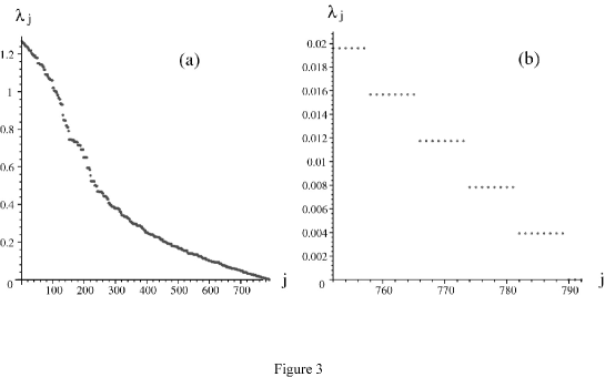
Figure 3: Lyapunov spectrum in the case of $(N_{1},N_{2})=(11,9)$. (a) Full scale. (b) Large $j$ part.

We can investigate the relation between a symmetry of the system and the step structure in the Lyapunov spectrum another way. For this purpose we consider the Lyapunov spectra in the square case and the rectangular case with the same number of particles. Here, the square system has the symmetry for the exchange of the vertical and the horizontal directions, which the rectangular system does not have. Fig. 4 is the Lyapunov spectra in the case of $(N_{1},N_{2})=(12,12)$ (the upper two graphs) and in the case $(N_{1},N_{2})=(24,6)$ (the lower two graphs) with $v=1.8$ and $\tau=2.3$. These graphs show that there is not a remarkable difference in the global shapes of the Lyapunov spectrum in these two cases, but the square system has (even twice) longer steps in the Lyapunov spectrum than in the rectangular system, shown in Figs. 4 (b) and (d). These longer steps come from an additional symmetry in the square system. Actually we can check numerically that the Lyapunov exponents obtained from the reduced matrix (102) are invariant under $k\leftrightarrow l$, which leads to more degeneracy in the case $N_{1}=N_{2}=12$ than when $(N_{1},N_{2})=(24,6)$. For $N_{1}=N_{2}$ all that is required is that $n_{1}$ and $n_{2}$ are interchanged. For $(N_{1},N_{2})=(24,6)$ degeneracy by this mechanism only occurs if $n_{1}$ is divisible by $4$ which is much rarer.

It should be noted that some steps of the Lyapunov spectra are too close to be distinguished in Fig. 4. For example, if we can investigate more precisely, we can see 5 different steps in the long flat part of the Lyapunov exponents $\lambda_{j}$ in $j\in[1018,1097]$ (in $j\in[1086,1125]$) in the Lyapunov spectrum in the case of $(N_{1},N_{2})=(12,12)$ (in the case of $(N_{1},N_{2})=(24,6)$). Similarly, most of the Lyapunov exponents $\lambda_{j}$, $j\in[1106,1152]$ ($j\in[1130,1152])$) in the case of $(N_{1},N_{2})=(12,12)$ (in the case of $(N_{1},N_{2})=(24,6)$) are not zero, just too small for the scale of the plot.

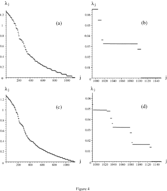
Figure 4: Lyapunov spectra in the cases of a square system $(N_{1},N_{2})=(12,12)$ ((a) Full scale. (b) Large $j$ part.) and a rectangular system $(N_{1},N_{2})=(24,6)$ ((c) Full scale. (d) Large $j$ part.).

5 Conclusion and Remarks

In this paper we have investigated the Lyapunov spectrum of a periodic orbit of a two-dimensional system, which consists of many disks with hard-core interactions. The system has a rectangular shape (or a square shape in a special case), and we used periodic boundary conditions. By the block cyclic structure of the matrix, which describes the tangent space dynamics, the calculation of the Lyapunov exponents is simplified to the eigenvalue problems of reduced $16\times 16$ matrices however many particles. The reduced matrix is used to consider the relation between such a step structure and symmetries of the system, and to show the existence of the thermodynamic limit in the Lyapunov spectrum. In particular we showed that the difference of the aspect ratio of the system appears in the stepwise structure of the Lyapunov spectrum rather than in the global shape of the Lyapunov spectrum.

The Lyapunov spectrum of the periodic orbit discussed in this paper shows a step structure, but it should be noted that this step structure is different from the step structure obtained by the numerical work [3]. More systematic investigations of the Lyapunov spectra of periodic orbits may be requested to explain the numerical results.

It should be emphasized that there are many periodic orbits in which we can calculate their Lyapunov spectra in many-hard-disk systems by using the block cyclic technique shown in this paper. On the other hand we are still far from the position where we can calculate the general Lyapunov spectrum of the many hard disk system by using the periodic orbit expansion technique. One of the problems is that in many particle system we could not know how to systematically find all of the periodic orbits whose periods are less than a given length. In addition, the periodic orbits of many-panicle system are typically distributed continuously, not isolated from each other. These problems make the application of the periodic orbit expansion technique to the many-particle systems difficult, and not yet solved.

Appendix A Block Cyclic Structure and the Reduced Matrix

In this appendix we show that the eigenvalues of the matrix $M_{n_{p}}$ are equal to the eigenvalues of the matrices ${\cal M}(2\pi n_{1}/N_{1},2\pi n_{2}/N_{2})$, $n_{1}=1,2,\cdots,N_{1}$, $n_{2}=1,2,\cdots,N_{2}$, given by Eq. (102).

First we calculate the matrix $M_{n_{p}}$. We multiply the matrices $M_{j}^{(c)}M_{j}^{(f)}$, $j=1,2,3,4$ given by Eqs. (57), (65), (66) and (74), and obtain

$$M_{n_{p}}=\left(\begin{array}[]{cccccc}K_{0}&K_{1}&&&&K_{2}\\ K_{2}&K_{0}&K_{1}&&&\\ &K_{2}&K_{0}&K_{1}&&\\ &&\ddots&\ddots&\ddots&\\ &&&K_{2}&K_{0}&K_{1}\\ K_{1}&&&&K_{2}&K_{0}\end{array}\right)$$ (113)

where $K_{j}$, $j=0,1,2$ are defined by

$$K_{0}\equiv\left(\begin{array}[]{cc}L_{02}L_{01}+L_{21}L_{11}+L_{11}L_{21}&L_{02}L_{12}+L_{21}L_{02}\\ L_{01}L_{11}+L_{22}L_{01}&L_{01}L_{02}+L_{22}L_{12}+L_{12}L_{22}\end{array}\right)$$ (116)

$$K_{1}\equiv\left(\begin{array}[]{cc}L_{21}^{2}&\tilde{0}\\ L_{01}L_{21}+L_{12}L_{01}&L_{12}^{2}\end{array}\right)$$ (119)

$$K_{2}\equiv\left(\begin{array}[]{cc}L_{11}^{2}&L_{11}L_{02}+L_{02}L_{22}\\ \tilde{0}&L_{22}^{2}\end{array}\right)$$ (122)

with the matrices $L_{jk}\equiv Q_{j}P_{k}$ and $8N_{1}\times 8N_{1}$ null matrix $\tilde{0}$. Eq. (113) implies that the matrix $M_{n_{p}}$ has the block cyclic structure, so it is block-diagonalized by the orthogonal matrix $U(16N_{1},N_{2})$ introduced through

$$U(j,k)\equiv\frac{1}{\sqrt{k}}\left(\begin{array}[]{ccccc}I_{j}e^{2\pi i1\times 1/k}&I_{j}e^{2\pi i1\times 2/k}&\cdots&I_{j}e^{2\pi i1\times k/k}\\ I_{j}e^{2\pi i2\times 1/k}&I_{j}e^{2\pi i2\times 2/k}&\cdots&I_{j}e^{2\pi i2\times k/k}\\ \vdots&\vdots&&\vdots\\ I_{j}e^{2\pi ik\times 1/k}&I_{j}e^{2\pi ik\times 2/k}&\cdots&I_{j}e^{2\pi ik\times k/k}\end{array}\right)$$ (127)

with the $j\times j$ identical matrix $I_{j}$ so that we obtain the matrix $U(16N_{1},N_{2})^{\dagger}$ $M_{n_{p}}U(16N_{1},N_{2})$ $=\mbox{Diag}(A(2\pi 1/N_{2}),$ $A(2\pi 2/N_{2}),\cdots,A(2\pi N_{2}/N_{2})$ with ${\dagger}$ meaning to take its Hermitian conjugate. Here the matrix $A(l)$ is defined by

$$A(l)\equiv K_{0}+K_{1}e^{il}+K_{2}e^{-il}.$$ (128)

The eigenvalues of the matrix $M_{n_{p}}$ are equal to the eigenvalues of the matrices $A(2\pi n_{2}/N_{2})$, $n_{2}=1,2,\cdots,N_{2}$.

The matrix $A(l)$ is represented as

$$A(l)=\left(\begin{array}[]{cc}B^{(1)}(l)&B^{(2)}(l)\\ B^{(3)}(l)&B^{(4)}(l)\end{array}\right)$$ (131)

where $B^{(j)}(l)$ is defined by

$$B^{(j)}(l)\equiv\left(\begin{array}[]{cccccc}B^{(j)}_{0}(l)&B^{(j)}_{1}(l)&&&&B^{(j)}_{2}(l)\\ B^{(j)}_{2}(l)&B^{(j)}_{0}(l)&B^{(j)}_{1}(l)&&&\\ &B^{(j)}_{2}(l)&B^{(j)}_{0}(l)&B^{(j)}_{1}(l)&&\\ &&\ddots&\ddots&\ddots&\\ &&&B^{(j)}_{2}(l)&B^{(j)}_{0}(l)&B^{(j)}_{1}(l)\\ B^{(j)}_{1}(l)&&&&B^{(j)}_{2}(l)&B^{(j)}_{0}(l)\end{array}\right).$$ (138)

Here the matrices $B^{(j)}_{k}(l)$, $j=1,2,3,4$ and $k=0,1,2$ are defined by

$$B^{(1)}_{0}(l) \equiv \left(\begin{array}[]{c}(\tilde{F}_{2}\tilde{F}_{1})^{2}+(\tilde{G}_{2}\tilde{G}_{1})^{2}+(\tilde{G}_{2}\tilde{F}_{1})^{2}e^{-il}\\ \tilde{F}_{2}\tilde{F}_{1}\tilde{F}_{2}\tilde{G}_{1}+\tilde{G}_{2}\tilde{G}_{1}\tilde{G}_{2}\tilde{F}_{1}+\tilde{G}_{2}\tilde{F}_{1}\tilde{G}_{2}\tilde{G}_{1}e^{il}\end{array}\right.$$ (144)

$$\hskip 28.45274pt\left.\begin{array}[]{c}\tilde{F}_{2}\tilde{F}_{1}\tilde{F}_{2}\tilde{G}_{1}+\tilde{G}_{2}\tilde{G}_{1}\tilde{G}_{2}\tilde{F}_{1}+\tilde{G}_{2}\tilde{F}_{1}\tilde{G}_{2}\tilde{G}_{1}e^{-il}\\ (\tilde{F}_{2}\tilde{F}_{1})^{2}+(\tilde{G}_{2}\tilde{G}_{1})^{2}+(\tilde{G}_{2}\tilde{F}_{1})^{2}e^{il}\end{array}\right)$$

$$B^{(1)}_{1}(l)\equiv\left(\begin{array}[]{cc}\hat{0}&\hat{0}\\ \tilde{F}_{2}\tilde{G}_{1}\tilde{F}_{2}\tilde{F}_{1}&(\tilde{F}_{2}\tilde{G}_{1})^{2}\\ \end{array}\right)$$ (147)

$$B^{(1)}_{2}(l)\equiv\left(\begin{array}[]{cc}(\tilde{F}_{2}\tilde{G}_{1})^{2}&\tilde{F}_{2}\tilde{G}_{1}\tilde{F}_{2}\tilde{F}_{1}\\ \hat{0}&\hat{0}\\ \end{array}\right)$$ (150)

$$B^{(2)}_{0}(l) \equiv \left(\begin{array}[]{c}\tilde{F}_{2}\tilde{F}_{1}\tilde{G}_{2}\tilde{F}_{1}+(\tilde{G}_{2}\tilde{F}_{1}\tilde{F}_{2}\tilde{F}_{1}+\tilde{F}_{2}\tilde{G}_{1}\tilde{G}_{2}\tilde{G}_{1})e^{-il}\\ \tilde{G}_{2}\tilde{G}_{1}\tilde{F}_{2}\tilde{F}_{1}\end{array}\right.$$ (156)

$$\hskip 28.45274pt\left.\begin{array}[]{c}\tilde{G}_{2}\tilde{G}_{1}\tilde{F}_{2}\tilde{F}_{1}e^{-il}\\ \tilde{F}_{2}\tilde{G}_{1}\tilde{G}_{2}\tilde{G}_{1}+\tilde{G}_{2}\tilde{F}_{1}\tilde{F}_{2}\tilde{F}_{1}+\tilde{F}_{2}\tilde{F}_{1}\tilde{G}_{2}\tilde{F}_{1}e^{-il}\end{array}\right)$$

$$B^{(2)}_{1}(l)\equiv\left(\begin{array}[]{cc}\tilde{G}_{2}\tilde{G}_{1}\tilde{F}_{2}\tilde{G}_{1}e^{-il}&\hat{0}\\ \tilde{F}_{2}\tilde{G}_{1}\tilde{G}_{2}\tilde{F}_{1}+\tilde{G}_{2}\tilde{F}_{1}\tilde{F}_{2}\tilde{G}_{1}+\tilde{F}_{2}\tilde{F}_{1}\tilde{G}_{2}\tilde{G}_{1}e^{-il}&\hat{0}\\ \end{array}\right)$$ (159)

$$B^{(2)}_{2}(l)\equiv\left(\begin{array}[]{cc}\hat{0}&\tilde{F}_{2}\tilde{F}_{1}\tilde{G}_{2}\tilde{G}_{1}+(\tilde{G}_{2}\tilde{F}_{1}\tilde{F}_{2}\tilde{G}_{1}+\tilde{F}_{2}\tilde{G}_{1}\tilde{G}_{2}\tilde{F}_{1})e^{-il}\\ \hat{0}&\tilde{G}_{2}\tilde{G}_{1}\tilde{F}_{2}\tilde{G}_{1}\\ \end{array}\right)$$ (162)

$$B^{(3)}_{0}(l) \equiv \left(\begin{array}[]{c}\tilde{F}_{2}\tilde{F}_{1}\tilde{G}_{2}\tilde{F}_{1}+(\tilde{F}_{2}\tilde{G}_{1}\tilde{G}_{2}\tilde{G}_{1}+\tilde{G}_{2}\tilde{F}_{1}\tilde{F}_{2}\tilde{F}_{1})e^{il}\\ \tilde{F}_{2}\tilde{G}_{1}\tilde{G}_{2}\tilde{F}_{1}+\tilde{G}_{2}\tilde{F}_{1}\tilde{F}_{2}\tilde{G}_{1}+\tilde{F}_{2}\tilde{F}_{1}\tilde{G}_{2}\tilde{G}_{1}e^{il}\end{array}\right.$$ (168)

$$\hskip 28.45274pt\left.\begin{array}[]{c}\tilde{F}_{2}\tilde{F}_{1}\tilde{G}_{2}\tilde{G}_{1}+(\tilde{F}_{2}\tilde{G}_{1}\tilde{G}_{2}\tilde{F}_{1}+\tilde{G}_{2}\tilde{F}_{1}\tilde{F}_{2}\tilde{G}_{1})e^{il}\\ \tilde{F}_{2}\tilde{G}_{1}\tilde{G}_{2}\tilde{G}_{1}+\tilde{G}_{2}\tilde{F}_{1}\tilde{F}_{2}\tilde{F}_{1}+\tilde{F}_{2}\tilde{F}_{1}\tilde{G}_{2}\tilde{F}_{1}e^{il}\end{array}\right)$$

$$B^{(3)}_{1}(l)\equiv\left(\begin{array}[]{cc}\hat{0}&\hat{0}\\ \tilde{G}_{2}\tilde{G}_{1}\tilde{F}_{2}\tilde{F}_{1}&\tilde{G}_{2}\tilde{G}_{1}\tilde{F}_{2}\tilde{G}_{1}\\ \end{array}\right)$$ (171)

$$B^{(3)}_{2}(l)\equiv\left(\begin{array}[]{cc}\tilde{G}_{2}\tilde{G}_{1}\tilde{F}_{2}\tilde{G}_{1}e^{il}&\tilde{G}_{2}\tilde{G}_{1}\tilde{F}_{2}\tilde{F}_{1}e^{il}\\ \hat{0}&\hat{0}\\ \end{array}\right)$$ (174)

$$B^{(4)}_{0}(l) \equiv \left(\begin{array}[]{c}(\tilde{F}_{2}\tilde{F}_{1})^{2}+(\tilde{G}_{2}\tilde{G}_{1})^{2}+(\tilde{G}_{2}\tilde{F}_{1})^{2}e^{il}\\ \tilde{F}_{2}\tilde{G}_{1}\tilde{F}_{2}\tilde{F}_{1}\end{array}\right.$$ (180)

$$\hskip 28.45274pt\left.\begin{array}[]{c}\tilde{F}_{2}\tilde{G}_{1}\tilde{F}_{2}\tilde{F}_{1}\\ (\tilde{F}_{2}\tilde{F}_{1})^{2}+(\tilde{G}_{2}\tilde{G}_{1})^{2}+(\tilde{G}_{2}\tilde{F}_{1})^{2}e^{-il}\end{array}\right)$$

$$B^{(4)}_{1}(l)\equiv\left(\begin{array}[]{cc}(\tilde{F}_{2}\tilde{G}_{1})^{2}&\hat{0}\\ \tilde{F}_{2}\tilde{F}_{1}\tilde{F}_{2}\tilde{G}_{1}+\tilde{G}_{2}\tilde{G}_{1}\tilde{G}_{2}\tilde{F}_{1}+\tilde{G}_{2}\tilde{F}_{1}\tilde{G}_{2}\tilde{G}_{1}e^{-il}&\hat{0}\\ \end{array}\right)$$ (183)

$$B^{(4)}_{2}(l)\equiv\left(\begin{array}[]{cc}\hat{0}&\tilde{F}_{2}\tilde{F}_{1}\tilde{F}_{2}\tilde{G}_{1}+\tilde{G}_{2}\tilde{G}_{1}\tilde{G}_{2}\tilde{F}_{1}+\tilde{G}_{2}\tilde{F}_{1}\tilde{G}_{2}\tilde{G}_{1}e^{il}\\ \hat{0}&(\tilde{F}_{2}\tilde{G}_{1})^{2}\end{array}\right)$$ (186)

with the $4\times 4$ null matrix $\hat{0}$. It follows from Eqs. (127), (131) and (138) that

$$\mbox{Diag}(U(8,N_{1}),U(8,N_{1}))^{\dagger}A(l)\;\mbox{Diag}(U(8,N_{1}),U(8,N_{1}))$$

$$=\left(\begin{array}[]{cc}C^{(1)}(l)&C^{(2)}(l)\\ C^{(3)}(l)&C^{(4)}(l)\end{array}\right)$$ (189)

where $C^{(j)}(l)$, $j=1,2,3,4$ are defined by $C^{(j)}(l)\equiv\mbox{Diag}($ $D^{(j)}(2\pi 1/N_{1},l),$ $D^{(j)}(2\pi 2/N_{1},l),$ $\cdots,D^{(j)}(2\pi N_{1}/N_{1},l)$ $)$ with $D^{(j)}(k,l)\equiv B^{(j)}_{0}$ $+B^{(j)}_{1}e^{ik}$ $+B^{(j)}_{2}e^{-ik}$. The matrix ${\cal M}(k,l)$ is introduced as

$${\cal M}(k,l)=\left(\begin{array}[]{cc}D^{(1)}(k,l)&D^{(2)}(k,l)\\ D^{(3)}(k,l)&D^{(4)}(k,l)\end{array}\right),$$ (192)

which is equal to Eq. (102). Therefore the eigenvalues of the matrix $A(l)$ are equal to the eigenvalues of the matrices ${\cal M}(2\pi n_{1}/N_{1},l)$, $n_{1}=1,2,\cdots,N_{1}$. It implies that the eigenvalues of the matrix $M_{n_{p}}$ are equal to the eigenvalues of the matrices ${\cal M}(2\pi n_{1}/N_{1},$ $2\pi n_{2}/N_{2})$, $n_{1}=1,2,\cdots,N_{1}$, $n_{2}=1,2,\cdots,N_{2}$.

References

[1]D. J. Evans and G. P. Morriss, “Statistical mechanics of
non-equilibrium liquids”, (Academic, London, 1990).
[2]N. Simanyi, mp_arc/01-300.
[3]H. A. Posch and R. Hirschl, in “Hard ball systems and the
Lorentz gas”, EMS Vol 101, Ed. D. Szasz (Springer, Berlin, 2000).
[4]C. P. Dettmann, ibid.
[5]D. Abraham and J. E. Marsden, “Foundations of Mechanics”,
2nd ed. (Benjamin/Cummins, Reading Mass., 1978).
[6]D. J. Evans, E. G. D. Cohen and G. P. Morriss, Phys. Rev.
A 42, 5990 (1990).
[7]C. P. Dettmann and G. P. Morriss, Phys. Rev. E 53,
R5545 (1996).
[8]C. P. Dettmann and G. P. Morriss, Phys. Rev. E 54,
2495 (1996).
[9]M. P. Wojtkowski and C. Liverani, Commun. Math. Phys.
194, 47 (1998).
[10]G. Benettin, L. Galgani, A. Giorgilli and J. M. Strelcyn,
C. R. Acad. Sci., Ser. A 286, 431 (1978).
[11]I. Shimada and T. Nagashima, Prog. Theor. Phys. 61, 1605
(1979).
[12]W. G. Hoover and H. A. Posch, J. Chem. Phys. 87, 6665 (1987).
[13] Ch. Dellago, H. A. Posch and W. G. Hoover, Phys. Rev. E 53,
1485 (1996).
[14]C. M. Newman, Commun. Math. Phys. 103, 121 (1986).
[15]R. Livi, A. Politi, S. Ruffo, and A. Vulpiani, J. Stat. Phys.
46, 147 (1987).
[16]Ya. G. Sinai, Int. J. Bifurcations Chaos Appl. Sci. Eng.
6, 1137 (1996).
[17]D. J. Searles, D. J. Evans and D. J. Isbister, Physica 240A,
96 (1997).
[18]L. Milanović, H. A. Posch and W. G. Hoover, Chaos 8,
455 (1998).
[19]J.-P. Eckmann and O. Gat, J. Stat. Phys. 98, 775 (2000).
[20] P. Cvitanović, R. Artuso, R. Mainieri, G. Tanner and
G. Vattay, “Classical and quantum chaos”
www.nbi.dk/ChaosBook/ (Niels Bohr Institute, Copenhagen, 2001).
[21] R. Artuso, E. Aurell and P. Cvitanović, Nonlinearity 3,
325 (1990); 3, 361 (1990).
[22] P. Cvitanović, P. Gaspard and T. Schreiber, Chaos 2,
85 (1992).
[23]W. N. Vance, Phys. Rev. Lett. 69, 1356 (1992).
[24]G. P. Morriss and L. Rondoni, J. Stat. Phys. 75, 553 (1994).
[25]P. Cvitanović, J.-P. Eckmann and P. Gaspard, Chaos, Solitons,
Fractals 6, 113 (1995).
[26]F. Christiansen, P. Cvitanović and V. Putkaradze, Nonlinearity
10, 55 (1997).
[27]L. Rondoni and G. P. Morriss, J. Stat. Phys. 86, 991 (1997).
[28]L. Rondoni and E. G. D. Cohen, Nonlinearity 11, 1395 (1998).
[29]R. E. Amritkar, P. M. Gade, A. D. Gangal and V. M. Nandkumaran
Phys. Rev. A 44, R3407 (1991).
[30]P. M. Gade and R. E. Amritkar, Phys. Rev. E 47, 143 (1993).