Efficiency of a stirred chemical reaction in a closed vessel

Abstract

We perform a numerical study of the reaction efficiency in a closed vessel. Starting with a little spot of product, we compute the time needed to complete the reaction in the container following an advection-reaction-diffusion process. Inside the vessel it is present a cellular velocity field that transports the reactants. If the size of the container is not very large compared with the typical length of the velocity field one has a plateau of the reaction time as a function of the strength of the velocity field, $U$. This plateau appears both in the stationary and in the time-dependent flow. A comparison of the results for the finite system with the infinite case (for which the front speed, $v_{f}$, gives a simple estimate of the reacting time) shows the dramatic effect of the finite size.

Numerous physical, biological and chemical systems show the propagation of a stable phase into an unstable one [1, 2]. When this phenomenon takes place in a fluid, one generally speaks of front propagation in advection-reaction-diffusion (ARD) systems. Under this generic name one indicates many different processes, e.g., the propagation of plankton populations in ocean currents [3], the transport of reacting pollutants in the atmosphere (e.g. ozone) [4], or the premixed combustion [5].

In the last years much effort has been done to study the influence of an advection field on the front dynamics. In particular, it is well established that the front speed in a laminar or turbulent fluid is enhanced with respect to the propagation in a medium at rest [6, 7]. In the context of (premixed) combustion processes the flame front area is proportional to the front speed and, therefore, an increasing of the front area due to the fluid stirring gives rise to an enhancement of the burning efficiency, that is, the system burns faster.

It is important to note that most of the theoretical studies and, in particular, the above results about the enhancement of burning efficiency, have been shown for an infinite-size system (in the propagation direction). Moreover, in order to introduce well-defined mathematical quantities one is forced to work with an infinite (or with periodic boundary conditions) system. This is the case of the front speed, which is an asymptotic quantity well defined only for an infinite system.

However, from a practical point of view one usually has to treat cases where the size of the domain is not much larger than the typical length scale of the velocity field [8]. The spreading of organisms in a lake or in a small closed sea basin, or the combustion of fuel in a machine motor are two clear examples where this may happen and, therefore, non-asymptotic properties can be very important [9, 10].

In this work we treat the case of an ARD process confined in a closed area. Beginning with a small quantity of material in the stable phase (in the following called burnt material), we numerically compute the time needed for a given percentage of the total area to be also burnt (called in the following, the reacting or burning time). The velocity field is of cellular flow type, that is, formed by circulating cells of fluid. Both, the stationary and the chaotic time-dependent cellular flow will be considered. Our main result, obtained either for the time-independent and for the time-dependent flow, is that increasing the typical velocity of the field one has a saturation of the burning rate. This saturation happens when the advection time scale is much faster than the reaction time scale. Also, we compare our results with the infinite-size case, studying the crossover from finite size systems to the asymptotic regime. We observe that the relevance of the system size is more important than expected a priori.

Let us consider the simplest non trivial case described by a scalar field $\theta({\bf x},t)$ which represents the concentration of reaction products, such that $\theta$ is equal one in the space-time coordinates where the reaction is over (the stable phase), and $\theta$ is zero where there is fresh material (the unstable phase). The dynamical evolution of this field is given by

$$\partial_{t}\theta+{\bf v}\cdot\nabla\theta=D\nabla^{2}\theta+\frac{f(\theta)}{\tau},$$ (1)

where ${\bf v}({\bf x},t)$ is the two-dimensional velocity field, $D$ is the diffusion coefficient, and $f(\theta)$ is the reaction term, where $\tau$ is the time scale for the reaction activity. For the reaction term we use the Fisher-Kolmogorov-Petrovskii-Piskunov (FKPP) nonlinearity [11], $f(\theta)=\theta(1-\theta)$. Concerning the velocity field, ${\bf v}$, we first adopt a simple stationary incompressible two-dimensional flow defined by the stream function

$$\psi(x,y)=\frac{UL}{\pi}\sin({\pi x\over L})\sin({\pi y\over L}),$$ (2)

being the parameter $U$ the maximum vertical velocity of the flow, and $L$ the size of one cell. For a study of the transport properties in the field (2) see ref. [12]; the asymptotic behaviour of front propagation is discussed in ref. [13]. The equations of motion for a fluid element are given by

$$\left\{{\begin{array}[]{lcr}\dot{x}&=&\partial_{y}\psi\\ \dot{y}&=&-\partial_{x}\psi.\end{array}}\right.$$ (3)

In this work the reaction processes described by (1) take place in a closed recipient. This confinement is implemented by assuming rigid boundary conditions on the box $0\leq y\leq L$ and $0\leq x\leq nL$, where $n$ is the number of circulating cells of the flow. One approaches to the asymptotic case increasing the value of $n$.

The settling of the problem is completed when we indicate the initial conditions, i.e., an initial spot of burnt material which starts the reaction. Thus, we use in all our numerical experiments a small circle of radius $r$ filled with stable material ($\theta=1$), that is placed at the initial time in the box filled with unstable material ($\theta=0$). The initial coordinates of the center of this circle are $(x=r,y=L/2)$ (the circle is on the border of the box; this mimic the injection of reacting material from the outside). As anticipated, the principal observable under investigation is the time needed for a given percentage of the total area to be burnt. We define $S(t)=\frac{1}{\Delta S}\int_{\Delta S}{\mathrm{d}}x{\mathrm{d}}y\theta(x,y,t)$ as the percentage of area burnt at time $t$, where $\Delta S=L^{2}n$ is the total area of the container. In our case, by choosing an appropriate $r$ the initial burnt material is $S(0)=0.005/n$, which is the $0.5\%$ of one cell. The reacting or burning time $t_{\alpha}$ is defined as the time needed for the percentage $\alpha$ of the total area of the recipient to be burnt, i.e., $S(t_{\alpha})=\alpha$.

Numerically, to integrate (1) we use the Feynman-Kac (FK) or stochastic Lagrangian approach. In this algorithm the field evolution is computed using the Lagrangian propagator plus a Montecarlo integration for the diffusive term. Then, the reaction propagator accounts for the reacting term (for details see [13, 14]). We also impose a rigid wall condition in the boundaries, in order to avoid that any fluid particle leaves the container, which could happen due to the noise term added to the velocity field in the Lagrangian approach.

We first show in Fig. (1) the influence of the velocity on the reacting efficiency, when different percentages, $\alpha$, of the final burnt area are considered.

FIG. 1.: $t_{\alpha}$ against the flow strength $U$ with $\tau=0.4$, $n=1$ and for various $\alpha$: $\alpha=0.2$ $(+)$, $\alpha=0.5$ $(\times)$, $\alpha=0.7$ $(\Box)$, $\alpha=0.9$ $(\circ)$.

Increasing the velocity of the flow, $U$, $t_{\alpha}$ decreases monotonically until a plateau is reached. Then, a further increasing of the flow velocity ($U>15$, similar for different $\alpha^{\prime}s$) does not decrease the burning time $t_{\alpha}$. We remark that this effect also appears for different finite values of the system size (different $n$’s), and different chemical rates $\tau$. At first glance, the appearance of the plateau seems to be surprising: in a closed container and for very high stirring intensity, increasing further more this intensity there is not an enhancement in the burning front propagation, that is, one does not improve the efficiency of burning.

The existence of the plateau can be understood noting that it is reached only when the reaction time, $\tau$, is large compared with the advection time, $\tau_{a}=L/U$. In this case, in the first stages of the process the active material invades the whole container because of advection and diffusion. Then the reaction term is the final responsible for the cell burning.

A direct comparison between the finite and the infinite system is interesting. In Fig. (2) we show the burning time scaled with the system size, i.e., $t_{\alpha}/n$, against the typical flow velocity, $U$, for some values of $n$. We also we plot the data obtained for an infinite system, which have been calculated from the front speed $v_{f}$ of the infinite system data according to

$$t_{\alpha}\simeq\frac{nL}{v_{f}},$$ (4)

which is expected to hold for $\alpha$ close to $1$ and large $n$.

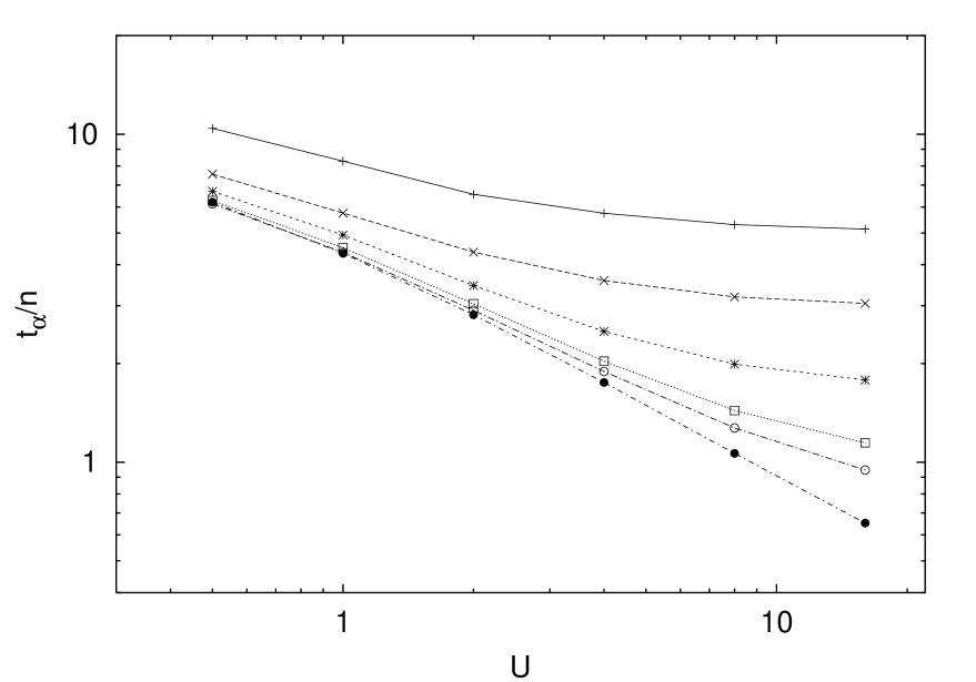
FIG. 2.: The burning time per unit-cell, $t_{\alpha}/n$, at various $U$ for $\tau=0.4$ and $\alpha=0.9$. The plots are for different system’s sizes: $n=1$ $(+)$, $n=2$ $(\times)$, $n=4$ $(*)$, $n=8$ $(\Box)$ and $n=12$ ($\circ$). It is also shown ($\bullet$) the burning time calculated using the front speed: $t=nL/v_{f}$.

Figure (2) shows that the asymptotic reacting time (given by $v_{f}$) is reached only in the large size limit, i.e., $n$ large, while the dynamics of small systems is dominated by the non asymptotic properties of the evolution.

Since the considered bidimensional velocity field (2) is stationary the Lagrangian trajectories are not chaotic. Nevertheless also in the case of Lagrangian chaotic trajectories, obtained with a time-dependent flow, the burning time shows the same qualitative behaviours shown in figures (1) and (2). Let us consider a time dependent flow whose streamfunction is

$$\psi(x,y,t)=U\sin(x+B(x)\cos(\omega t))\sin(y)\,.$$ (5)

This is sufficient to induce Lagrangian chaos [16] in the evolution of passive tracers advected by the velocity field (3) generated by (5). Because we are dealing with closed systems $B(x)$ is constructed in such a way that it is zero near the boundary of the system and almost constant, $B_{0}$, otherwise: $B(x)=B_{0}(1-\exp(-1/x)-\exp(-1/(nL-x)))$.

FIG. 3.: $t_{\alpha}$ against the flow strength $U$ for various $\alpha$ in the unsteady case ($B=1.1$ and $\omega=2.09$): $\alpha=0.2$ $(+)$, $\alpha=0.5$ $(\times)$, $\alpha=0.7$ $(\Box)$, $\alpha=0.9$ $(\circ)$. The flow is confined in two cells.

In Fig. (3) we show the curve $t_{\alpha}$ against $U$ for different values of $\alpha$. At difference from the previous case, when unsteady flow is concerned there is not a simple plateau in $t_{\alpha}$, but an oscillatory behaviour due to the interplay between the oscillation period of the separatrices and the circulation time inside the cell. It happens that circulation and oscillation “synchronize” producing a very efficient and coherent way of transferring passive particles from one cell to the other. A similar, but much more impressive, feature occurs for the effective diffusion coefficient in the horizontal direction [17]. Anyway, for low values of $U$ the mixing induced by the time dependence makes that the system burns quite faster. For higher $U$, the mixing properties of the flow are not sufficient to improve furthermore the burning efficiency, and at the end, the typical time for the cell burning is proportional to the reaction time-scale.

Summing up, the physical mechanism of reaction in a closed recipient for both time-independent and time-dependent cellular flows are quite similar. When the typical time-scale of the velocity field, $L/U$, is larger than the reaction time-scale, $\tau$, the initial condition is quickly spread along the whole system due to advection (and diffusion), in such a way that in all the container the value of $\theta$ is small but different from zero. Then, basically only reaction plays an important role, and a further increasing of the flow velocity does not decrease the burning time.

Let us study the dependence of the saturation time $t_{\alpha}^{s}(\tau)$, which is the value of the burning time in the plateau, as a function of $\tau$. In the unsteady case, we choose the minimum value of $t_{\alpha}$ at varying $U$ as the saturation time.

In Figure (4) we show the result for the unsteady case, which can be interpreted following the same arguments used to explain the existence of the plateau. Essentially the burning process in the case of large $U$ can be divided in two steps, the initial mixing regime and the reacting dominated regime. In fact, from the initial condition (in which only a small fraction of the volume is active) one has a rapid spreading (say in a time $\tilde{t}$) because of advection and diffusion. After the spreading one has an exponential increasing of the field due to the reaction term. The time $\tilde{t}$ is expected to be a decreasing function of $U$ (with a limiting value for sufficiently large $U$). This implies, together with a dimensional argument, $t_{\alpha}^{s}(\tau)=\tilde{t}+b_{\alpha}\tau$. Thus, there is a linear dependence of $t_{\alpha}^{s}$ with $\tau$ as shown in Figure (4), which has been obtained for the time-dependent flow, but similar results hold also for the steady case.

FIG. 4.: Plot of $t_{\alpha}^{s}(\tau)$ vs $\tau$ at various percentages of filling $\alpha$ in the time-dependent case ($B=1.1$ and $\omega=2.09$): $\alpha=0.2$ $(+)$, $\alpha=0.5$ $(\times)$, $\alpha=0.7$ $(\Box)$, $\alpha=0.9$ $(\circ)$. For each curve we have superimposed the linear fit $t_{\alpha}^{s}(\tau)=\tilde{t}+b_{\alpha}\tau$, where $\tilde{t}$ and $b_{\alpha}$ are fitting parameters. Here $n=2$.

The value of the slope of the saturation time against $\tau$, $b_{\alpha}$, can be analytically studied. We have that, in the regime of very high $U$ such that the plateau is reached, after the time $\tilde{t}$ the initial condition is spread out through the whole container and one can approximate $\theta(x,y,t)\sim\tilde{\theta}(t)$, being $\tilde{\theta}(t)$ a rough average of the $\theta$ field in the container, which evolves following only the reaction part of (1). This is because, as we have argued before, after $\tilde{t}$ the important physical mechanism of burning comes from the chemical activity and not from the mixing due to the advection and diffusion. Then $S(t)=\tilde{\theta}(t)$ for $t>\tilde{t}$, and so:

$$\frac{{\mathrm{d}}S}{{\mathrm{d}}t}={1\over\tau}S(1-S).$$ (6)

This can be integrated from $\tilde{t}$ to $t$, taking into account that we can approximate $S(\tilde{t})\sim S(0)$, i.e., the initial condition is just spread out in the system in the initial stages of the process. One has that

$$\log\left(\frac{S(t)}{1-S(t)}\right)-\log\left(\frac{S(0)}{1-S(0)}\right)=\frac{t-\tilde{t}}{\tau}\,\,.$$ (7)

Finally, as $S(t_{\alpha}^{s})=\alpha$ we get

$$t_{\alpha}^{s}=\tilde{t}+\tau\log\left(\frac{\alpha(1-S(0))}{(1-\alpha)S(0)}\right)\equiv\tilde{t}+b_{\alpha}\tau\,\,,$$ (8)

which gives the dependence of $b_{\alpha}$ on the percentage of burnt material, $\alpha$.

For the time-independent cellular flow the reasonings follow closely the former ones. In fact, in the regime of large $U$, when all over the cell (by diffusion) there is also a small quantity of active reagent, the reaction process can begin with an averaged $S(t)$ (in a mean-field sense).

Despite the numerous approximations done to obtain (8), it is in excellent agreement with the numerical results, see Fig. (5), confirming once again the physical mechanism we think that give rise to the existence of the saturation time.

FIG. 5.: The slope, $b_{\alpha}$, of the saturation time $t_{\alpha}^{s}$ against $\tau$, that is, the slope of the curves in Fig. (4) (with an additional value for $\alpha=0.95$), vs the percentage $\alpha$. With $(\Box)$ the numerical values for time dependent flow, with $(*)$ the numerical value (rescaled) for steady flow, and with the solid line the prediction given by (8).

Summarizing, we have performed a numerical study of an advection-reaction-diffusion system confined in a closed vessel, using stationary and time dependent cellular flows. Beginning with a small quantity of the active phase, we have calculated the time needed for a percentage of the total area to be burnt. Thus, our numerical experiments may represent the spreading of an organism in a lake or the combustion of a material in a vessel. The main lesson to learn from our studies is that the influence of the system size has been shown to be very important [18]. In particular, we have shown that for very large flow velocities the reacting time saturates, giving rise to the unexpected result that increasing further more the flow velocity there is not a decreasing of the time to burn the material. We have to mention that a similar scenario, i.e., the appearance of the plateau in the burning time, has been obtained for other types of chemical reactions $f(\theta)$, like the Arrhenius $f(\theta)=(1-\theta)\exp(-\theta_{0}/\theta)$ ($\theta_{0}$ constant) or the Zeldovich function $f(\theta)=\theta^{m}(1-\theta)$, with $m=2$.

This work has been partially supported by INFM Parallel Computing Initiative and MURST (Cofinanziamento Fisica Statistica e Teoria della Materia Condensata). C.L. acknowledges support from MECD of Spain, D.V and A.V. acknowledge support from the INFM Center for Statistical Mechanics and Complexity (SMC).

REFERENCES

- [1] J. Xin, SIAM Review 42, 161 (2000).
- [2] J.D. Murray, Mathematical Biology, Springer-Verlag, Second Edition, (1993).
- [3] J.H. Steele (ed.), Spatial patterns in plankton communities, Plenum Press, New York (1978).
- [4] I. R. Epstein, Nature 374, 231 (1995).
- [5] N. Peters, Turbulent combustion, Cambridge University Press (2000).
- [6] P. Constantin, A. Kiselev, A. Oberman and L. Ryzhik, Arch. Rational Mechanics 154, 53 (2000).
- [7] A. Kiselev and L. Ryzhik, Ann. I.H. Poincaré 18, 309 (2001).
- [8] G. Boffetta, A. Celani, M. Cencini, G. Lacorata and A. Vulpiani, Chaos 10, 50 (2000).
- [9] P. Rys, Chimia 46, 469 (1992).
- [10] A. Gorczakowski, A. Zawadzki, J. Jarosinski and B. Veyssiere, Combust. Flame 120, 359 (2000).
-
[11]
A. N. Kolmogorov, I. G. Petrovskii, and N. S. Piskunov,
Moscow Univ. Bull. Math. 1, 1 (1937);
R. A. Fischer, Ann. Eugenics 7, 355 (1937). - [12] T.H. Solomon and J.P. Gollub, Phys. Rev. A 38, 6280 (1988).
- [13] M. Abel, A. Celani, D. Vergni and A. Vulpiani, Phys. Rev. E 64, 046307 (2001).
- [14] U. Frisch, A. Mazzino, A. Noullez and M. Vergassola, Phys. Fluids 11, 2178 (1999).
- [15] M. V. Tretyakov and S. Fedotov, Physica D 159, 190 (2001).
-
[16]
H. Aref, J. Fluid Mech. 143, 1 (1984);
A. Crisanti, M. Falcioni, G. Paladin and A. Vulpiani, Riv. Nuovo Cimento 14, 1 (1991). - [17] P. Castiglione, A. Crisanti, A. Mazzino, M. Vergassola and A. Vulpiani, J. Phys. A 31, 7197 (1998).
- [18] A different phenomenon where the influence of the system size is also very important is reported in M. V. Tretyakov and S. Fedotov, Physica D 159, 190 (2001).