Electromigration-Induced Propagation of Nonlinear Surface Waves

Abstract

Due to the effects of surface electromigration, waves can propagate over the free surface of a current-carrying metallic or semiconducting film of thickness $h_{0}$. In this paper, waves of finite amplitude, and slow modulations of these waves, are studied. Periodic wave trains of finite amplitude are found, as well as their dispersion relation. If the film material is isotropic, a wave train with wavelength $\lambda$ is unstable if $\lambda/h_{0}<3.9027\ldots$, and is otherwise marginally stable. The equation of motion for slow modulations of a finite amplitude, periodic wave train is shown to be the nonlinear Schrödinger equation. As a result, envelope solitons can travel over the film’s surface.

I. Introduction

Waves propagating over the free surface of a layer of water subject to gravity have been studied extensively for well over a century. In his ground breaking paper of 1847, Stokes showed that steady periodic wave trains of finite amplitude are possible, and that their dispersion relation depends upon their amplitude Stokes . In these wave trains, the effects of dispersion and nonlinearity balance, yielding a steady wave form.

In the 1960’s, it was discovered that if the water is of finite depth $h_{0}$ and the wavelength $\lambda=2\pi/k$ is sufficiently short, the wave train is unstable. Benjamin and Feir BF showed that the Stokes wave train is unstable to small modulational or side band perturbations if $kh_{0}>1.363\ldots$, and this been confirmed experimentally Benjamin ; Yuen ; Lake ; Shemer .

Benjamin and Feir’s analysis holds only at early times, just after the instability has begun to develop. Zakharov Zakharov and later Hasimoto and Ono HO derived an equation of motion for the envelope of a packet of finite-amplitude gravity waves which remains valid long after the onset of the instability. Their equation — the nonlinear Schrödinger equation — admits envelope soliton solutions that are intimately related to the ultimate state of the fluid surface.

Although it is not yet widely appreciated, there are nontrivial electrical free boundary problems. When an electrical current passes through a piece of solid metal or semiconductor, collisions between the conduction electrons and the atoms at the surface lead to drift of these atoms. This phenomenon, which is known as surface electromigration (SEM), can cause the surface of a solid to move and deform Latyshev ; Stoyanov ; Krug_and_Dobbs ; Kraftapl ; Suojap ; Mohanjap ; Krug1 ; Krug2 ; Gengor1 ; Gengor2 ; Gengor3 ; Mohanepl ; Mohanpre . The free surface of a conducting film moves in response to the electrical current flowing through the bulk of the film, in much the same way that flow in the bulk of a fluid affects the motion of its surface. However, the analogy is not perfect — the boundary conditions are very different in the two problems. In addition, metals and semiconductors are anisotropic materials, and this distinguishes them from fluids as well.

Waves can propagate over the free surface of a current-carrying film deposited on an insulating substrate, at least in the limit of small amplitude. These waves, whose propagation is induced by surface electromigration, are somewhat analogous to gravity waves, and will be called “SEM waves.” The linear dispersion relation for these waves has been known for some time Krug1 , and will be discussed briefly in Sec. III.

It is natural to ask to what extent the nonlinear behavior of gravity waves is paralleled by that of SEM waves. To address this question, in this paper I will study SEM waves of finite amplitude, and slow modulations of these waves. Periodic wave trains of finite amplitude (the analog of the Stokes wave) are found, as well as their dispersion relation. If the film material is isotropic, the wave trains are unstable for $kh_{0}>1.609927\ldots$ and are otherwise marginally stable. The equation of motion for slow modulations of the finite amplitude, periodic wave train is shown to be the nonlinear Schrödinger equation.

It is worth mentioning that SEM is not just of academic interest: In modern integrated circuits, the current-carrying metal lines or “interconnects” carry very high current densities, and electrical failure can occur due to the effects of SEM. In particular, SEM can cause a small perturbation at the edge of a metal strip to become a slit-shaped void which propagates across the line until its tip contacts the opposite side of the strip; electrical failure is then complete Mohanepl ; Mohanpre ; Rose ; Sanchezapl .

II. Equations of Motion

Consider a single-crystal metallic or semiconducting film of uniform thickness $h_{0}$ deposited on the plane surface of an insulating substrate. We take the $z$ axis to be normal to the film-vacuum interface and locate the origin $O$ in this plane. (We will occasionally find it convenient to use another set of Cartesian coordinates $(x^{\prime},z^{\prime})$ with $x^{\prime}=x$, $z^{\prime}=z+h_{0}$ and origin $O^{\prime}$ at the substrate surface.) The film’s surface $z=0$ will be assumed to be a low index crystal plane. A constant electrical current flows through the film in the $x$ direction, and the electric field within the film is $\vec{E}_{0}=E_{0}\hat{x}$.

Now suppose that the upper surface of the film is perturbed. Let the outward-pointing unit normal to this surface be $\hat{n}$. For simplicity, we shall restrict our attention to perturbations whose form does not depend upon $y$, so that the height of the film’s surface above the substrate $h=h_{0}+\zeta$ depends only on $x$ and $t$ (Fig. 1). The upper film surface will evolve in the course of time due to the effects of SEM and surface self-diffusion. We assume that the current flowing through the film is held fixed.

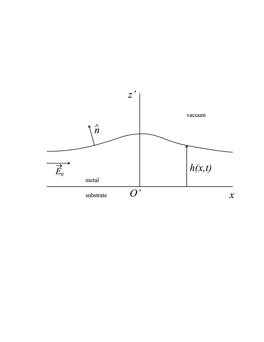
Figure 1: The current-carrying metal thin film. The height of the free surface above the substrate, $h$, depends only on $x$ and $t$. The outward-pointing unit normal to the free surface is $\hat{n}$, and the electric field far from the perturbation is $\vec{E}_{0}$.

Clearly, the problem is two-dimensional (2D), and the dependence of all quantities on $y$ will therefore be suppressed. The electrical potential $\Phi=\Phi(x,z,t)$ satisfies the 2D Laplace equation

$$\nabla^{2}\Phi=0$$ (1)

and is subject to the boundary condition $\hat{n}\cdot\vec{\nabla}\Phi=0$ on the upper surface and $\hat{z}\cdot\vec{\nabla}\Phi=0$ on the lower. More explicitly, we have

$$\Phi_{z}(x,\zeta,t)=\zeta_{x}\Phi_{x}(x,\zeta,t)$$ (2)

and

$$\Phi_{z}(x,-h_{0},t)=0,$$ (3)

where $f_{x}\equiv\partial f/\partial x$ and so forth. If the initial perturbation is localized, we also have

$$\zeta\to 0$$ (4)

for $x\to\pm\infty$ and, furthermore,

$$\vec{\nabla}\Phi(x,z,t)\to-\vec{E}_{0}$$ (5)

for $x\to\pm\infty$ and $-h_{0}\leq z\leq 0$.

We assume that the atomic mobility is negligible at the film-insulator interface, so that the form of that interface remains planar for all time. Further, in the interest of simplicity, we assume that the applied current is high enough that the effects of SEM are much more important than those of capillarity. The surface atomic current $\vec{J}_{a}$ is then proportional to the electrical current at the surface. Explicitly, $\vec{J}_{a}=-\nu Mq\vec{\nabla}\Phi$, where the $\nu$ is the areal density of the mobile surface atoms, $q$ is their effective charge, and $M$, the adatom mobility, in general depends on the surface slope $\zeta_{x}$. When there is a net influx of atoms into a small surface element, it will move. The normal velocity of the film’s free surface is $v_{n}=q\nu\Omega\partial_{s}(M\partial_{s}\Phi)$, where $\Omega$ is the atomic volume and $s$ is the arc length along the surface. Therefore

$$\zeta_{t}=q\nu\Omega\partial_{x}\left[{{M(\zeta_{x})}\over{\sqrt{1+\zeta_{x}^{2}}}}\partial_{x}\Phi(x,\zeta,t)\right],$$ (6)

where $\partial_{x}$ is the total derivative with respect to $x$. (Since $\zeta$ depends on $x$, we have $\partial_{x}\Phi(x,\zeta,t)=\Phi_{x}(x,\zeta,t)+\zeta_{x}\Phi_{z}(x,\zeta,t)$, for example.) Together, Eqs. (1) - (6) completely describe the nonlinear dynamics of the film surface.

III. Finite Amplitude Periodic Wave Trains

We wish to study the propagation of a disturbance whose amplitude is small. To this end, we put $\Phi=-E_{0}x+\phi$ and presume that $\zeta$ and $\phi$ are of order $\epsilon$.

We shall suppose that the crystal structure is invariant under the reflection $x\to-x$, so that $M$ is an even function of the slope $\zeta_{x}$. As a result, $M(\zeta_{x})=M_{0}(1+c\zeta_{x}^{2})+O(\epsilon^{4})$, where $M_{0}\equiv M(0)$ and $c$ is a dimensionless constant which vanishes for an isotropic material.

If we work to order $\epsilon$, the equations of motion are linearized and we find that sinusoidal waves of the form $\zeta=2a\cos(kx-\omega_{0}t)$ propagate over the surface. $\omega_{0}=\omega_{0}(k)$ is given by the linear dispersion relation

$$\omega_{0}=-\beta E_{0}{{k^{2}}\over\sigma},$$ (7)

where $\beta\equiv qM_{0}\nu\Omega$ and $\sigma\equiv\tanh kh_{0}$ Krug1 . The corresponding group velocity is

$$v_{g}=v_{0}\left[h_{0}^{2}k^{2}\left(1-{1\over{\sigma^{2}}}\right)+2{h_{0}k\over\sigma}\right],$$ (8)

where $v_{0}=-\beta E_{0}/h_{0}$ is the phase velocity of waves of infinitely long wavelength. If the amplitude $2a$ is not a constant but instead varies slowly with position, the resulting amplitude modulation will propagate with the group velocity.

The goal of this paper is to go beyond the linear approximation and study wave trains of finite amplitude. To begin, we will find the analog of the Stokes wave propagating over deep water: we will consider the limit $h_{0}\to\infty$ and restrict our attention to periodic wave trains with constant amplitude $a$. These simplifying assumptions will be relaxed in the next section.

Expanding $\zeta$ and $\phi$ in powers of the amplitude, we have

$$\zeta=[a{\cal E}+\mu_{2}a^{2}{\cal E}^{2}+\mu_{3}a^{3}{\cal E}^{3}+\ldots]+{\rm c.c.}$$ (9)

and

$$\phi=[\nu_{1}ae^{kz}{\cal E}+\nu_{2}a^{2}e^{2kz}{\cal E}^{2}+\nu_{3}a^{3}e^{3kz}{\cal E}^{3}+\tilde{\nu}_{3}a^{3}e^{kz}{\cal E}+\ldots]+{\rm c.c.},$$ (10)

where ${\cal E}\equiv e^{i(kx-\omega t)}$, “c.c.” denotes the complex conjugate, and $\mu_{2}$, $\mu_{3}$, $\nu_{1}$, $\nu_{2}$, $\nu_{3}$ and $\tilde{\nu}_{3}$ are constants to be determined. We can take $a$ to be real without loss of generality. $\omega$ must depend on $a$ if the appearance of secular terms at the third order is to be avoided. Again expanding in powers of $a$, we have

$$\omega=\omega_{0}+a^{2}\omega_{2}+\ldots,$$ (11)

where $\omega_{0}=-\beta E_{0}k^{2}$ is the linear dispersion relation for $h_{0}\to\infty$ and $\omega_{2}=\omega_{2}(k)$.

Our expansion for $\phi$ satisfies the Laplace equation. Since we are seeking a periodic wave train, the boundary conditions (4) and (5) do not apply. Inserting our expansions (9), (10) and (11) into Eqs. (2) and (6), setting $\alpha=1-2c$, and working to third order in $a$, we obtain

$$\omega_{2}=\beta E_{0}\left(1+{3\over 2}\alpha-\alpha^{2}\right)k^{4},$$ (12)

$$\mu_{2}={1\over 2}\alpha k,$$ (13)

$$\mu_{3}={1\over 4}\alpha(2\alpha-1)k^{2},$$ (14)

$$\nu_{1}=-iE_{0},$$ (15)

$$\nu_{2}=i\left(1-{1\over 2}\alpha\right)E_{0}k,$$ (16)

$$\nu_{3}=-{1\over 2}i\left(3-{{7\over 2}}\alpha+\alpha^{2}\right)E_{0}k^{2},$$ (17)

and

$$\tilde{\nu}_{3}={1\over 2}i(3\alpha-1)E_{0}k^{2}.$$ (18)

The nonlinear dispersion relation is

$$\omega=-\beta E_{0}k^{2}\left[1-\left(1+{3\over 2}\alpha-\alpha^{2}\right)k^{2}a^{2}+\ldots\right].$$ (19)

For the isotropic case $\alpha=1$, the magnitude of the phase velocity

$$v_{p}\equiv{\omega\over k}=-\beta E_{0}k\left(1-{3\over 2}k^{2}a^{2}+\ldots\right)$$ (20)

is a decreasing function of $a$ when $a$ is small. In contrast, the phase velocity of small amplitude gravity waves on deep water increases with amplitude. For a given amplitude $2a$, the phase velocity is smallest for $\alpha=3/4$, or, equivalently, for $c=1/8$.

The form of the periodic wave train is given by

$$\zeta=2a\cos(kx-\omega t)+\alpha ka^{2}\cos 2(kx-\omega t)+{1\over 2}\alpha(2\alpha-1)k^{2}a^{3}\cos 3(kx-\omega t)+\ldots$$ (21)

To third order in $a$, the wave is symmetric about the crests, even though the applied electric field breaks the right-left symmetry.

IV. Slow Modulation of Finite Amplitude Periodic Wave Trains

We will now relax the simplifying assumptions of Section III. Suppose $h_{0}$ is finite and that the amplitude is a slowly varying function of position. We set

$$\zeta=\sum_{n=-\infty}^{\infty}\zeta_{n}E^{n}$$ (22)

and

$$\phi=\sum_{n=-\infty}^{\infty}\phi_{n}E^{n},$$ (23)

where $E\equiv e^{i(kx-\omega_{0}t)}$ and $\omega_{0}$ is given by the linear dispersion relation for films of finite thickness, Eq. (7). Since $\zeta$ and $\phi$ are real, $\zeta_{-n}=\zeta_{n}^{\ast}$ and $\phi_{-n}=\phi_{n}^{\ast}$ for all $n$.

Because the amplitude of the wave is of order $\epsilon$, the coefficients $\zeta_{n}$ and $\phi_{n}$ are of order $\epsilon^{n}$. We may therefore write

$$\zeta_{n}=\sum_{j=n}^{\infty}\epsilon^{j}\zeta_{nj}$$ (24)

and

$$\phi_{n}=\sum_{j=n}^{\infty}\epsilon^{j}\phi_{nj}.$$ (25)

Here $n\geq 0$ and the $\zeta_{nj}$’s and $\phi_{nj}$’s do not depend on $\epsilon$. Note as well that $\zeta_{00}=\phi_{00}=0$ and that the $\zeta_{0j}$’s and $\phi_{0j}$’s are all real.

To find a steady, periodic wave train (the analog of the Stokes wave), we would take the amplitudes $\zeta_{nj}$ to be constants and the $\phi_{nj}$’s to depend on $z$ alone. We will go further, and allow the $\zeta_{nj}$’s to vary slowly in space and time as viewed from the frame of reference moving with the group velocity. As a result, we will be able to find the steady, periodic wave train and investigate its stability as well. (Our analysis closely parallels Davey and Stewartson’s treatment of modulated gravity waves DS .) To be explicit, we set

$$\zeta_{nj}=\zeta_{nj}(\xi,\tau)$$ (26)

and

$$\phi_{nj}=\phi_{nj}(\xi,z,\tau),$$ (27)

where $\xi\equiv\epsilon(x-v_{g}t)$ and $\tau\equiv\epsilon^{2}t$. The method of multiple scales will be employed, i.e., $x$, $\xi$, $t$, and $\tau$ will be treated as independent variables. Using the chain rule, we see that

$${d\over{dx}}={\partial\over{\partial x}}+\epsilon{\partial\over{\partial\xi}}$$ (28)

and

$${d\over{dt}}={\partial\over{\partial t}}-\epsilon v_{g}{\partial\over{\partial\xi}}+\epsilon^{2}{\partial\over{\partial\tau}}.$$ (29)

We now insert our expansions for $d/dx$ and $\phi$ into the Laplace equation (1). This results in a series of ordinary differential equations for the $\phi_{nj}$’s. Applying the boundary condition (3), we find that

$$\phi_{11}=A{{\cosh kz^{\prime}}\over{\cosh kh_{0}}},$$ (30)

$$\phi_{22}=F{{\cosh 2kz^{\prime}}\over{\cosh 2kh_{0}}},$$ (31)

$$\phi_{12}=G{{\cosh kz^{\prime}}\over{\cosh kh_{0}}}-iA_{\xi}{{z^{\prime}\sinh kz^{\prime}}\over{\cosh kh_{0}}},$$ (32)

and

$$\phi_{13}=-{1\over 2}A_{\xi\xi}(z^{\prime})^{2}{{\cosh kz^{\prime}}\over{\cosh kh_{0}}}-iG_{\xi}z^{\prime}{{\sinh kz^{\prime}}\over{\cosh kh_{0}}}+H{{\cosh kz^{\prime}}\over{\cosh kh_{0}}},$$ (33)

where $A$, $F$, $G$ and $H$ depend only on $\xi$ and $\tau$. It also follows that $\phi_{01}$ and $\phi_{02}$ are functions of $\xi$ and $\tau$ alone, while

$${{\partial\phi_{03}}\over{\partial z}}=-z^{\prime}{{\partial^{2}\phi_{01}}\over{\partial\xi^{2}}}.$$ (34)

The next step is quite laborious but is nonetheless straightforward, and so I will omit the details. Inserting our expansions for $d/dx$, $d/dt$, $\zeta$ and $\phi$ into Eqs. (2) and (6) and working to second order in $\epsilon$, we find that

$$\zeta_{01}=0,$$ (35)

$$\zeta_{11}=i{{\sigma}\over{E_{0}}}A,$$ (36)

$$\zeta_{12}=i{{\sigma}\over{E_{0}}}G+{{h_{0}}\over{E_{0}}}A_{\xi},$$ (37)

$$\zeta_{22}=-{k\over{\sigma E_{0}^{2}}}\left[1-\left(1-{1\over 2}\alpha\right)\sigma^{2}\right]A^{2}$$ (38)

and

$$F={{ik}\over{2E_{0}\sigma^{2}}}(1+\sigma^{2})\left[1-\left(2-{1\over 2}\alpha\right)\sigma^{2}\right]A^{2}.$$ (39)

Equating the coefficient of $\epsilon^{3}E^{0}$ to zero in Eqs. (2) and (6) yields two linear equations for $\zeta_{02}$ and $\partial\phi_{01}/\partial\xi$. Solving these for $\zeta_{02}$, we obtain

$$\zeta_{02}=\left({{\sigma k}\over{E_{0}^{2}}}\right){{\alpha\sigma h_{0}k-2}\over{v_{g}/v_{0}-1}}|A|^{2}.$$ (40)

When we equate the coefficient of $\epsilon^{3}E^{1}$ to zero in Eqs. (2) and (6), we obtain two equations that are consistent only if

$$iA_{\tau}=\Gamma A_{\xi\xi}+\Lambda|A|^{2}A,$$ (41)

where the constants $\Gamma$ and $\Lambda$ are given by

$$\Gamma=-{1\over 2}{{d^{2}\omega_{0}}\over{dk^{2}}}={{\beta E_{0}}\over\sigma}\left(1+2\sigma h_{0}k-{{v_{g}}\over{v_{0}}}\right)$$ (42)

and

$$\Lambda={{\beta k^{4}}\over{\sigma E_{0}}}\left[{2\over{\sigma^{2}}}-1-\alpha+\left({5\over 2}\alpha-\alpha^{2}\right)\sigma^{2}-\left(1-\sigma^{2}+{\sigma\over{h_{0}k}}\right){{2v_{g}/v_{0}-\alpha\sigma h_{0}k}\over{v_{g}/v_{0}-1}}\right].$$ (43)

Eq. (41) is the nonlinear Schrödinger equation, and describes the time development of the amplitude modulation. It has nonlinear plane wave solutions

$$A=A_{0}e^{i(\Omega\tau-\kappa\xi)},$$ (44)

where $A_{0}$ and $\kappa$ are constants and $\Omega=\Gamma\kappa^{2}-\Lambda|A_{0}|^{2}$. Let us recast the solution with $\kappa=0$ in terms of the original, physical variables. For $\kappa=0$, Eq. (37) has the solution $\zeta_{12}=G=0$, and we will specialize to this case. We set $\sigma\epsilon A_{0}=-iE_{0}a$, where $a$ is a real constant of order $\epsilon$. To second order in $a$,

$$\zeta=2a\cos(kx-\omega t)+\left({k\over\sigma}\right){{\alpha\sigma h_{0}k-2}\over{v_{g}/v_{0}-1}}a^{2}+{{2k}\over{\sigma^{3}}}\left[1-\left(1-{1\over 2}\alpha\right)\sigma^{2}\right]a^{2}\cos 2(kx-\omega t),$$ (45)

where

$$\omega=\omega_{0}+\Lambda\left({{E_{0}}\over\sigma}\right)^{2}a^{2}.$$ (46)

Eq. (45) describes a periodic wave train of finite amplitude propagating over a metal or semiconducting layer of finite thickness. Eq. (46) is the nonlinear dispersion relation.

In the limit $h_{0}k\gg 1$, Eq. (45) becomes

$$\zeta=2a\cos(kx-\omega t)+\alpha ka^{2}\cos 2(kx-\omega t)+{1\over 2}\alpha ka^{2}+\ldots$$ (47)

and Eq. (46) reduces to Eq. (19). Eq. (47) reduces to Eq. (21) after a trivial vertical shift of the origin, and so the results of this section have the correct thick film limit.

For $h_{0}k\ll 1$, Eq. (45) is

$$\zeta=2a\cos(kx-\omega t)-{2\over{h_{0}^{3}k^{2}}}a^{2}\left[1-\cos 2(kx-\omega t)\right]+\ldots$$ (48)

where

$$\omega=v_{0}k\left(1+{1\over 3}h_{0}^{2}k^{2}+{2\over{h_{0}^{4}k^{2}}}a^{2}+\ldots\right).$$ (49)

Eqs. (48) and (49) are valid for $ka\ll(kh_{0})^{3}\ll 1$. It has been shown elsewhere soliton that the equation of motion for small amplitude, long waves is the Korteweg-de Vries (KdV) equation

$$\zeta_{t}=-v_{0}\zeta_{x}+{1\over 3}v_{0}h_{0}^{2}\zeta_{xxx}+2{v_{0}\over{h_{0}}}\zeta\zeta_{x}.$$ (50)

The KdV equation has finite amplitude, periodic solutions (cnoidal waves) of the form

$$\zeta=-2a+4a\,{\rm cn}^{2}[\pi^{-1}K(m)(kx-\omega t)|m],$$ (51)

where cn is a Jacobian elliptic function, $K(m)$ is the complete elliptic integral of the first kind,

$$\omega=v_{0}k\left[1+{{4a}\over{3h_{0}}}\left({2\over m}-1\right)\right],$$ (52)

and $m$ is given implicitly by the following relation:

$$mK^{2}(m)={{2\pi^{2}a}\over{h_{0}^{3}k^{2}}}.$$ (53)

Eqs. (51) - (53) give a good approximate solution to the original equations of motion in the limit that $a/h_{0}$ and $h_{0}k$ tend to zero with $a/h_{0}^{3}k^{2}$ remaining finite as the limit is taken. If the amplitude of the cnoidal wave is small enough that $ka\ll(kh_{0})^{3}\ll 1$, Eqs. (51) and (52) reduce to Eqs. (48) and (49). Thus, in the thin film limit, the nonlinear wave (45) is a cnoidal wave of small amplitude.

The periodic wave train (44) is marginally stable if $\Gamma\Lambda\leq 0$ but is unstable if $\Gamma\Lambda>0$ HO . This means that for a given value of $\alpha$, the periodic wave train is unstable if $kh_{0}$ exceeds a critical value we shall denote by $\chi_{c}=\chi_{c}(\alpha)$, and is marginally stable for $kh_{0}\leq\chi_{c}$. The critical value $\chi_{c}=1.609927\ldots$ for the isotropic case ($\alpha=1$) and is infinite for $\alpha\geq 2$ and $\alpha\leq-1/2$. Fig. 2 is a plot of $1/\chi_{c}(\alpha)$ as a function of $\alpha$. It is intereresting to note that the smallest value of $\chi_{c}$ is obtained for a value of $\alpha$ differing just slightly from unity ($\alpha=0.972\ldots$).

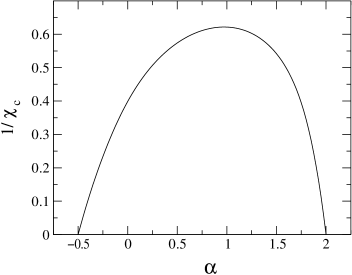
Figure 2: A plot of $1/\chi_{c}$ as a function of $\alpha$. $\chi_{c}^{-1}$ is zero for $\alpha\geq 2$ and $\alpha\leq-1/2$.

For $kh_{0}\ll 1$, the product $\Gamma\Lambda$ is negative, regardless of the value of $\alpha$. The periodic wave train is therefore marginally stable in this limit. This is in accord with the fact that cnoidal waves are marginally stable Drazin .

IV. Conclusions

In this paper, the electromigration-induced dynamics of small-amplitude disturbances on a low index crystal surface were studied. Periodic wave trains of finite amplitude were found, as well as their dispersion relation. These wave trains are unstable for $kh_{0}>\chi_{c}(\alpha)$, and are otherwise marginally stable. The value of the parameter $\alpha$ depends on strength of the material anisotropy, and is equal to 1 if the anisotropy is negligible. For $\alpha=1$, $\chi_{c}=1.609927\ldots$. For $\alpha\leq-1/2$ and $\alpha\geq 2$, on the other hand, $\chi_{c}$ is infinite and the wave train is marginally stable no matter what its wavelength.

The equation of motion for slow modulations of the finite amplitude, periodic wave train was shown to be the nonlinear Schrödinger equation. As is well known, this equation is exactly solvable for initial conditions that vanish with sufficient speed as $|x|\to\infty$ ZS . This exact solution has an number of consequences for electromigration-induced propagation of surface waves. If $kh_{0}>\chi_{c}(\alpha)$, a localized initial wave packet of arbitrary shape will eventually disintegrate into a number of envelope solitons and a small oscillatory tail. These solitons survive collisions with each other with no permanent change except a shift in phase and position.

What are the prospects of an experimental test of the theory developed in this paper? Quite recently, the SEM-induced dynamics of metal surfaces of large area have received some attention, but unfortunately these experiments were carried out on polycrystalline films, and so they do not permit a test of the theory Shimoni ; Shimoni2 .

The experimental situation is more promising in the case of semiconductors. A number of beautiful experimental studies of the SEM-induced dynamics of single crystal silicon films have been carried out, but on initially planar, vicinal surfaces Latyshev ; bunching . These studies revealed that a vicinal surface is unstable against step-bunching for one current direction, and that it is stable for the opposite current direction. Experimental studies of the dynamics of perturbed, low-index silicon surfaces that are subject to high electric fields have not yet been carried out.

To test the theory, a singly-periodic periodic wave structure could be etched into a low-index silicon surface. After perturbing the surface in this way, a high electrical current would be applied parallel to the ripple wavevector. The subsequent surface dynamics could be imaged by scanning tunneling microscopy, as has already been done for vicinal surfaces.

The analog of the Stokes wave would be obtained by etching many parallel ripples into the wafer surface before the application of current. In this way, the amplitude dependence of the phase velocity could be determined and compared with the theoretical prediction. To observe the development of an envelope soliton (or solitons), on the other hand, a few tens or hundreds of ripples would be etched into the film initially. This would produce a “wave packet” that would ultimately disintegrate into one or more envelope solitons and a small oscillatory tail under the action of an applied current.

References

- (1) G. G. Stokes, Camb. Trans. 8, 441 (1847).
- (2) T. B. Benjamin and J. E. Feir, J. Fluid Mech. 27, 417 (1967).
- (3) T. B. Benjamin, Proc. Roy. Soc. A 299, 59 (1967).
- (4) H. C. Yuen and B. M. Lake, Phys. Fluids 18, 956 (1975).
- (5) B. M. Lake and H. C. Yuen, J. Fluid Mech. 83, 75 (1977).
- (6) L. Shemer, E. Kit, H. Jiao and O. Eitan, J. Waterway Port Coastal Ocean Eng. 124, 320 (1998).
- (7) V. E. Zakharov, Sov. Phys. J. Appl. Mech. Technol. Phys. 4, 190 (1968).
- (8) H. Hasimoto and H. Ono, J. Phys. Soc. Japan 33, 805 (1972).
- (9) A. V. Latyshev, A. L. Aseev, A. B. Krasilnikov and S. I. Stenin, Surf. Sci. 213, 157 (1989).
- (10) S. Stoyanov, Jpn. J. Appl. Phys. 29, L659 (1990); ibid 30, 1 (1991).
- (11) J. Krug and H. T. Dobbs, Phys. Rev. Lett. 73, 1947 (1994).
- (12) O. Kraft and E. Arzt, Appl. Phys. Lett. 66, 2063 (1995); Acta Materialia 45, 1599 (1997).
- (13) W. Wang, Z. Suo, and T. H. Hao, J. Appl. Phys 79, 2394 (1996).
- (14) M. Mahadevan and R. M. Bradley, J. Appl. Phys 79, 6840 (1996).
- (15) M. Schimschak and J. Krug, Phys. Rev. Lett. 78, 278 (1997).
- (16) M. Schimschak and J. Krug, Phys. Rev. Lett. 80, 1674 (1998).
- (17) M. R. Gungor and D. Maroudas, Appl. Phys. Lett. 72, 3452 (1998).
- (18) M. R. Gungor and D. Maroudas, Surf. Sci. 415, L1055 (1998).
- (19) M. R. Gungor and D. Maroudas, J. Appl. Phys. 85, 2233 (1999).
- (20) M. Mahadevan, R. M. Bradley, and J.-M. Debierre, Europhys. Lett. 45, 680 (1999).
- (21) M. Mahadevan and R. M. Bradley, Phys. Rev. B 59, 11037 (1999).
- (22) J. H. Rose, Appl. Phys. Lett. 61, 2171 (1992).
- (23) J. E. Sanchez, Jr., O. Kraft, and E. Arzt, Appl. Phys. Lett. 61, 3121 (1992).
- (24) A. Davey and K. Stewartson, Proc. R. Soc. Lond. A 338, 101 (1974).
- (25) R. M. Bradley, Phys. Rev. E 60, 3736 (1999).
- (26) P. G. Drazin, Quart. J. Mech. Appl. Math. 30, 91 (1977).
- (27) V. E. Zakharov and A. B. Shabat, Sov. Phys. JETP 34, 62 (1972).
- (28) N. Shimoni, M. Wolovelsky, O. Biham and O. Millo, Surf. Sci. 380, 100 (1997).
- (29) N. Shimoni, S. Ayal and O. Millo, Phys. Rev. B 62, 13147 (2000).
- (30) For a review, see H.-C. Jeong and E. D. Williams, Surf. Sci. Reports 34, 171 (1999), Section 4.4.