Inverse Cascade Regime in Shell Models of 2-Dimensional Turbulence

Abstract

We consider shell models that display an inverse energy cascade similar to 2-dimensional turbulence (together with a direct cascade of an enstrophy-like invariant). Previous attempts to construct such models ended negatively, stating that shell models give rise to a “quasi-equilibrium” situation with equipartition of the energy among the shells. We show analytically that the quasi-equilibrium state predicts its own disappearance upon changing the model parameters in favor of the establishment of an inverse cascade regime with K41 scaling. The latter regime is found where predicted, offering a useful model to study inverse cascades.

The inverse energy cascade in 2-dimensional Navier-Stokes turbulence is an important phenomenon with implications for geophysical flows 67Kra . In addition, it had been found that correlation functions and structure functions obey very closely Kolmogorov scaling (so-called K41), with only minute anomalous corrections, in contradistinction to 3-dimensional turbulence in which intermittency corrections to K41 scaling are sizable 01Tab . This difference is well documented 93SY ; 98PT ; 00BCV but not yet understood. It is therefore tempting to construct simple models of the phenomenon. Indeed, several attempts were made to construct shell models for this purpose, 94ABCFPV ; 96DM . So far these attempts ended negatively, failing to find a statistical steady state in which energy flows from smaller to larger scales together with having a Kolmogorov energy spectrum. Rather, it was thought that whenever energy flew “backwards”, the statistical steady state settled close to thermodynamic equilibrium. In this letter we show that there actually exists a wide range of parameter values for which shell models display the wanted behavior, thereby offering useful testing grounds for ideas on 2-dimensional turbulence.

We discuss the issue in the framework of the Sabra shell model 98LPPPV . Like all shell models 98BJPV this represents a truncated Fourier representation of the Navier-Stokes equations. The Sabra model reads

$$\frac{du_{n}}{dt} = i(ak_{n+1}u_{n+1}^{*}u_{n+2}+bk_{n}u_{n-1}^{*}u_{n+1}$$ (1)

$$- ck_{n}u_{n-1}u_{n-2})-\gamma_{n}u_{n}+f_{n}\ ,$$

where the dissipative term $\gamma_{n}$ reads $\nu k_{n}^{2\alpha}+\mu k_{n}^{-2\beta}$, with $\nu$ and $\mu$ being the viscosity and drag coefficients respectively. Here $u_{n}$ are complex numbers standing for the Fourier components of the velocity field belonging to shell $n$, associated with wavenumbers $k_{n}$. The latter are restricted to the set $k_{n}=k_{0}\lambda^{n}$, with $\lambda$ being the spacing parameter, taken below to be 2. The forcing $f_{n}$ is chosen here to act at intermediate values of $n$, $n=n_{f}$, allowing in principle to study direct as well as inverse fluxes. The forcing is taken random with Gaussian time correlations as in 98LPPPV ; the amplitude of the forcing is fixed below to $1/\sqrt{2}$ in all cases. The dissipative terms $\gamma_{n}$ act both on the smallest and the largest scales with their respective (hyper)-viscosity and drag exponents $\alpha$ and $\beta$; below we use $\alpha=\beta=2$. The dissipative terms become dominant at the viscous and drag scales $n_{d}$ and $n_{L}$ respectively. We will always have $n_{L}\ll n_{f}\ll n_{d}$. The coefficients $a$, $b$ and $c$ are adjustable parameters, with the constraint $a+b+c=0$ ensuring the conservation of energy in the dissipationless limit. Choosing $a=1$ we explore the problem in terms of the single parameter $b$, with $-2<b<0$ 98LPPPV .

It was shown before 73Gle ; 88YO that for $b<-1$ there exist two positive definite invariants, the energy $E$ and the “enstrophy” $H$,

$$E=\frac{1}{2}\sum_{n=1}^{N}|u_{n}|^{2}\ ,\quad H=\frac{1}{2}\sum_{n=1}^{N}\Big{(}\frac{-1}{b+1}\Big{)}^{n}|u_{n}|^{2}\ ,$$ (2)

which, in this case, are associated with an inverse and direct fluxes respectively 94ABCFPV . However, the statistical steady state found in the regime $-5/4<b<-1$ in 94ABCFPV ; 96DM is close to thermodynamic equilibrium. This can be demonstrated via the properties of the structure functions, defined by

$$S_{2}(k_{n}) = \langle|u_{n}|^{2}\rangle\ ,$$ (3)

$$S_{3}(k_{n}) = \text{Im}\{\langle u_{n-1}u_{n}u_{n+1}^{*}\rangle\}\ ,$$ (4)

$$S_{4}(k_{n}) = \langle|u_{n}|^{4}\rangle\ ,$$ (5)

etc. Indeed, in 96DM these objects were found in the inertial range to be close to the exact solution in thermodynamic equilibrium which reads

$$S_{2}(k_{n}) = \frac{1}{B+A(a/c)^{n}}\ ,$$ (6)

$$S_{3}(k_{n}) = 0\ ,$$ (7)

$$S_{4}(k_{n}) = S_{2}(k_{n})^{2}\ ,\quad\text{etc.}$$ (8)

Formula (6) has two asymptotes: for small $n$ in agreement with energy equipartition, and for large $n$ with enstrophy equipartition.

$$S_{2}(k_{n}) \sim k_{n}^{0}\ ,\quad n_{L}\ll n\ll n_{c}\ ,$$ (9)

$$S_{2}(k_{n}) \sim \left(\frac{c}{a}\right)^{n}\ ,\quad n_{c}\ll n\ll n_{f}\ .$$ (10)

Here $n_{c}\approx\log(B/A)/\log(a/c)$ is the cross over shell separating the two asymptotic scaling forms of $S_{2}$. $A$ and $B$ are coefficients depending on the forcing and the dissipation. In particular, in this regime close to thermodynamic equilibrium, the cross over $n_{c}$ moves to higher shells when the viscosity $\nu$ is reduced. Unless otherwise stated, we choose parameters such that $n_{c}\ll n_{f}$.

Equation (7) implies zero fluxes. However in our simulations we find in this regime a finite inverse flux of energy and a direct flux of enstrophy which do not go to zero when $\gamma_{n}\to 0$. The fact that the fluxes do not vanish also implies that $S_{3}$ is not exactly zero. One can write down the exact form of $S_{3}$, which is correct always when there is a flux of energy or a flux of enstrophy :

$$S_{3}(k_{n}) \sim k_{n}^{-1}\ ,\>n_{L}\ll n\ll n_{f}\ \mbox{(energy flux),}$$ (11)

$$S_{3}(k_{n}) \sim k_{n}^{-1}\left(\frac{c}{a}\right)^{n}\ ,\>n_{f}\ll n\ll n_{d}\ \mbox{(enst. flux).}\$$ (12)

A measure of the deviation of the statistics from Gaussian behavior is provided by the ratio

$$R(k_{n})\equiv\frac{S_{3}(k_{n})}{S_{2}(k_{n})^{3/2}}\ ,$$ (13)

which according to Eqs. (6)-(12) has the three separate regimes

$$R(k_{n}) \sim k_{n}^{-1}\ ,\quad n_{L}\ll n\ll n_{c}\ ,$$ (14)

$$R(k_{n}) \sim k_{n}^{-1}\left(\frac{a}{c}\right)^{3n/2}\ ,\quad n_{c}\ll n\ll n_{f}\ ,$$ (15)

$$R(k_{n}) \sim k_{n}^{-1}\left(\frac{a}{c}\right)^{n/2}\ ,\quad n_{f}\ll n\ll n_{d}\ .$$ (16)

These regimes are illustrated in Fig. 1.

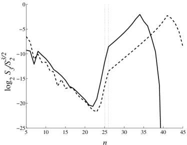
Figure 1: The ratio $R(k_{n})\equiv S_{3}(k_{n})/S_{2}(k_{n})^{3/2}$ as a function of $n$ for $b=-1.1$ and $\nu=10^{-43}$ (dashed line) and $\nu=10^{-33}$ (solid line). One clearly sees the three regimes predicted by Eqs. (14), (15), (16), with the minimum occurring at $n=n_{c}$. The minimum deepens and moves to higher shells when the viscosity is reduced. The vertical dotted lines designate the forcing scale. Note that at small values of $n$ the statistics converges on much longer time scales than for large values of $n$; hence the remnant fluctuations around the scaling prediction.

When $R$ is small, it provides a measure of the magnitude of the fluxes compared to their standard deviations. $R$ is of order of unity at the dissipative boundaries, while it reaches its minimal value at $n=n_{c}$. The former follows from the fact that the dissipative boundaries are precisely where the second order dissipative terms balance the third order transfer terms. In fact the ratio $R$ cannot be larger than unity whenever scaling prevails. One sees this directly from the definitions (3) and (4):

$$S_{3}(k_{n})/\sqrt{S_{2}(k_{n-1})S_{2}(k_{n})S_{2}(k_{n+1}})\leq 1\ .$$ (17)

Since $n_{c}$ moves to higher shells when the viscosity is reduced, the value of $R$ at the minimum decreases: we divide a decreasing $S_{3}$ by an $S_{2}$ that remains constant over a larger range of $n$. We thus conclude that the quasi-equilibrium regime displays a alphabetical small parameter when $\nu\to 0$. We will see that in the Kolmogorov regime there is only a numerical small parameter.

In ref. 96DM it was then discovered that there exists a transition for $b$ crossing a critical value ($b=-5/4$ for $\lambda=2$) after which $S_{2}$ gains a new form in the direct enstrophy flux regime, close to the Kraichnan dimensional prediction 67Kra

$$S_{2}(k_{n})\sim k_{n}^{-2[1+\log_{\lambda}(a/c)]/3}\ ,\quad n_{f}\ll n\ll n_{d}\ ,$$ (18)

(up to small corrections). We note that this prediction can be inferred from Eq. (16) and the condition (17). Indeed $R$ must be an increasing function of $n$ towards its small scale boundary, which yields

$$(a/c)\geq\lambda^{2}\Leftrightarrow b\geq-a\left(1+\frac{1}{\lambda^{2}}\right)\ ,$$ (19)

or $b\geq-5/4$ for $\lambda=2$ and $a=1$. Thus for $b<-5/4$ Eq. (16) can no longer be valid. While $S_{3}(k_{n})$ does not change, $S_{2}(k_{n})$ is replaced by the form (18) and consequently Eq. (16) is replaced by

$$R(k_{n})\sim k_{n}^{0},\ n_{f}\ll n\ll n_{d}\ (b<-5/4)\ .$$ (20)

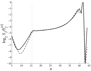
Figure 2: Same as Fig. 1 but for $b=-1.5$ (dot-dashed line) and $-1.6$ (solid line). One clearly sees the three regimes predicted by Eqs. (14), (15), (20). Note that the constant regime $k_{n}^{0}$ is still effected by finite size effects from the viscous end. However the two curves are essentially the same.

In Fig. 2 we present this ratio as computed from numerical simulations with the values of $b=-1.5$ and $-1.6$. We have used a total of 46 shells, with $\nu=10^{-37}$, $\mu=10^{-3}$. The forcing was on shells 15 and 16. The three regimes are clearly seen, with the added important confirmation that this ratio is of the order of unity at the two dissipative boundaries.

Nevertheless previous work failed to find a similar phenomenon for the range of scales that supports the inverse flux of energy. In that range the statistics remained close to thermodynamic equilibrium, leading to the common belief that shell models cannot be used to model 2-dimensional turbulence. We explain next that the statistical solution claimed for the regime $b<-5/4$, i. e. local thermodynamic equilibrium for the inverse flux of energy and direct enstrophy cascade, predicts its own destruction when $b$ is reduced further beyond a critical value $b_{c}$ that we can compute analytically. Indeed the set of Eqs. (14), (15), (20) and the condition (17) further implies that $R$ cannot be a decreasing function of $n$ in the range $n_{c}\ll n\ll n_{f}$, which implies

$$\left(\frac{a}{c}\right)^{3/2}\geq\lambda\Leftrightarrow b\geq-a(1+\lambda^{-2/3})\ .$$ (21)

Accordingly, for $b<b_{c}\equiv-a(1+\lambda^{-2/3})$ the quasi-equilibrium in the inverse energy flux regime can no longer be supported, and it changes into a true cascade regime with K41 scaling. For $\lambda=2$ this occurs at the critical value $b_{c}\approx-1.63$, where $S_{2}(k_{n})$ assumes the scaling form

$$S_{2}(k_{n})\sim k_{n}^{-2/3}\ ,\ n_{L}\ll n\ll n_{f}\ .$$ (22)

Note that Eq. (22) implies the collapse $n_{c}\to n_{L}$.

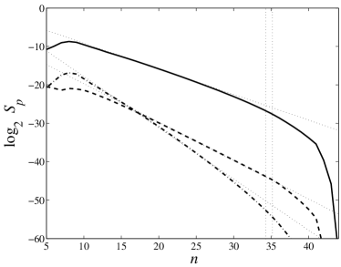
Figure 3: Second (solid line), third (dashed line) and fourth (dot-dashed line) order structure functions in the inverse cascade regime for $b=-1.9$. The vertical dotted lines indicate the forcing range $n_{f}=35,36$. The dotted lines have K41 slopes of -2/3, -1 and and -4/3 respectively.

In Fig. 3 we show the results of simulations at $b=-1.9$, with forcing at shells $n_{f}=35,\>36$ and otherwise the same parameter values as in Fig. 1. The agreement with K41 scaling is apparent. We note that the scaling laws (22) and (11) (which remains true in this regime) imply that $R(k_{n})$ becomes constant as a function of $k_{n}$. Thus we cannot display an alphabetical small parameter anymore. Nevertheless, the measurement of the constant value of $R$ in the inverse cascade regime yields a number of the order of 0.02 or less. We thus have a numerical small parameter, that is similar in magnitude to the corresponding value of $R$ in 2-dimensional turbulence 00BCV .

In summary, we exhibited a new regime of the statistical properties of shell models in which inverse energy cascade exists side by side with a direct enstrophy cascade. The statistical objects satisfy scaling laws in close correspondence with the Kraichnan dimensional predictions for 2-dimensional turbulence. Since this model is so much simpler than 2-dimensional Navier-Stokes equations, it should provide useful grounds to understand the phenomenon theoretically. Such a discussion and a more detailed account of our numerical findings will be presented elsewhere 02GLPP .

- (1) R. H. Kraichnan, Phys. Fluids 10, 1417 (1967).
- (2) P. Tabeling, Phys. Rep., in press.
- (3) L. M. Smith and V. Yakhot, Phys. Rev. Lett 71,352 (1993).
- (4) J. Paret and P. Tabeling, Phys. Fluids 10, 3126 (1998).
- (5) G. Boffetta, A. Celani and M. Vergassola, Phys. Rev. E 61, R29 (2000).
- (6) E. Aurell, G. Boffetta, A. Crisanti, P. Frick, G. Paladin, and A. Vulpiani, Phys. Rev. E 50, 4705 (1994).
- (7) P. D. Ditlevsen and I. A. Mogensen, Phys. Rev. E 53, 4785-4793 (1996).
- (8) V. S. L’vov, E. Podivilov, A. Pomyalov, I. Procaccia, and D. Vandembroucq, Phys. Rev. E 58, 1811 (1998).
- (9) T. Bohr, M. H. Jensen, G. Paladin, and A. Vulpiani, Dynamical Systems Approach to Turbulence, (Cambridge, 1998) and references therein.
- (10) E. B. Gledzer, Dokl. Akad. Nauk SSSR 209, 1046 (1973) [Sov. Phys. Dokl. 18, 216 (1973)].
- (11) M. Yamada and K. Ohkitani, Prog. Theo. Phys. 79, 1265 (1988).
- (12) T. Gilbert, V. S. L’vov, A. Pomyalov and I. Procaccia, in preparation.