Freely decaying weak turbulence for sea surface gravity waves

Abstract

We study numerically the generation of power laws in the framework of weak turbulence theory for surface gravity waves in deep water. Starting from a random wave field, we let the system evolve numerically according to the nonlinear Euler equations for gravity waves in infinitely deep water. In agreement with the theory of Zakharov and Filonenko, we find the formation of a power spectrum characterized by a power law of the form of $|{\bf k}|^{-2.5}$.

After the pioneering work by Kolmogorov [1] on the equilibrium range in the spectrum of an homogeneous and isotropic turbulent flow, there have been a number of studies on cascade processes in many other fields of classical physics such as plasma physics, magnetohydrodynamics and ocean waves. For surface gravity waves the first seminal theoretical work was done by O.M. Phillips in 1958, [2]. Using dimensional arguments, he argued that the frequency spectrum in the inertial range was of the form $F(\omega)=\alpha g^{2}\omega^{-5}$, where $\alpha$ was supposed to be an absolute constant and $g$ is gravity. Even though in the introduction of Phillips’ paper it was stated that “a necessary condition for the equilibrium range over a certain part of the spectrum is the appreciable non-linear interactions among these wave-numbers” (from [2]), his arguments were based on the geometrical features of the free surface elevation. One of his basic assumptions was that the only variable of interest was gravity, while the friction velocity, $u_{*}$, was not supposed to be involved in the spectral relation, limiting the possibility for a correct dimensional analysis.

Some years later Zakharov and Filonenko [3] established that in infinite water the direct cascade should produce a power spectrum of the surface elevation of the form $P(|{\bf k}|)\sim|{\bf k}|^{-2.5}$ that corresponds, using the linear dispersion relation in infinite depth, to an $\omega^{-4}$ frequency power spectrum: the result was found as an exact solution of the kinetic wave equation (see [4]). The theory developed is known as ”weak” or ”wave turbulence” and has many important applications in different fields of physics such as hydrodynamics, plasma physics, nonlinear optics, solid state physics, etc. see [5]. It is called weak turbulence because it deals with resonant interactions among small-amplitude waves. Thus, contrary to fully developed turbulence, it leads to explicit analytical solutions provided some assumptions are made. The first experimental support of the theory for surface gravity waves was made by Toba [6] who was completely unaware of the paper by Zakharov and Filonenko. He reformulated the Phillips’ equilibrium range law in the following way: $F(\omega)=\beta gu_{*}\omega^{-4}$, where $\beta$ should now be a universal dimensionless constant. After the work by Toba, successive experimental observation of the $\omega^{-4}$ law have been made by a number of authors, see for example [7, 8, 9, 10].

Even though there is a consensus on this result, it must be stressed that so far the verification of the theory has never been established from first principles and moreover the mechanisms that lead to the power law $\omega^{-4}$ are not universally recognized: geometrical aspects related to wave breaking, without invoking the nonlinear wave-wave interaction mechanism, are still retained by many oceanographers as fundamental for generating an $\omega^{-4}$ power law. Confirmation of the Zakharov-Filonenko solution to the kinetic equation has being given through numerical simulations of the kinetic wave equation itself [11] [12], solving exactly the so called $S_{nl}$ term. Nevertheless, it must be underlined that the kinetic equation is derived from the primitive equations of motion under a number of hypotheses (see for example [13]), therefore it cannot be concluded $a$ $priori$ that power law solutions of the kinetic equation are also shared by the fully nonlinear wave equations.

One way to verify weak turbulence theory is to perform direct numerical simulations of the primitive equations of motion. The numerical confirmation of the theory for gravity waves propagating on a surface has not been an easy task (for capillary waves see [14], for one dimensional wave turbulence see [15, 16]), basically because of the intrinsic difficulties of the computation of the boundary conditions. Different numerical approaches have been used for integrating the fully nonlinear surface gravity waves equations (see [17] for a review). The numerical methods based on volume formulations show very interesting results, in particular they are capable of modeling in a quite appropriate way wave breaking. Unfortunately they have the disadvantage that they require large computational resources, and therefore are not suitable for long time numerical simulations. For irrotational and inviscid flows boundary formulations are usually preferred: only the surface is discretized reducing the dimension of computation (from three to two). The Higher-Order Spectral Methods (HOS), indeed the method used in our numerical simulations, introduced independently by West et al. [18] and by Dommermuth et al. [19], belongs to this second approach (see also the recent work byTanaka [20]). Very recently three new methods have been proposed as very promising for simulating water waves [21, 22, 23]. Results using these new approaches on turbulent cascades are still to be completed.

In this Letter we establish numerically, using a HOS method, that nonlinear interactions are sufficient for generating power laws in wave spectra; moreover we show that the Zakharov-Filonenko theory is completely consistent with the primitive equations of motion. We consider a system of random waves localized in wave number space and we show how nonlinearities “adjust” the spectrum in agreement with the Zakharov and Filonenko prediction. Numerical work in the case of a forced and dissipated system has been attempted by Willemsen [24] using what sometimes are called the “Krasitskii equations” (see also [13]). In order to avoid the effects of external forcing, we considered the case of a freely decaying wave field. If the simulations, as we will see, show the formation of a power law then the conjecture that this power law is caused by geometrical features related to forcing and wave breaking must be excluded, since forcing is absent and wave breaking cannot be taken into account using the numerical method considered. From a physical point of view, the freely decaying case corresponds to the evolution of a swell wave field. A generic wave field is considered at time $t=0$ and it is allowed to evolve in a natural way using a high order approximation of the Euler equations. Since numerical computations are limited by the dimension of the grid considered, an artificial dissipation is needed at high wave numbers in order to prevent accumulation of energy and a break down of the numerical code. The fluid is considered inviscid, irrotational and incompressible. Under these conditions the velocity potential $\phi(x,y,z,t)$ satisfies the Laplace’s equation everywhere in the fluid. The boundary conditions are such that the vertical velocity at the bottom is zero and on the free surface the kinematic and dynamic boundary conditions are satisfied for the velocity potential $\psi(x,y,t)=\phi(x,y,\eta(x,y,t),t)$ (we assume that fluid is of infinite depth):

$${\psi_{t}+g\eta+\frac{1}{2}\bigg{[}\psi_{x}^{2}+\psi_{y}^{2}-(\phi_{z}|_{\eta})^{2}(1+\eta_{x}^{2}+\eta_{y}^{2})\bigg{]}=0}$$ (1)

$${\eta_{t}+\psi_{x}\eta_{x}+\psi_{y}\eta_{y}-\phi_{z}|_{\eta}(1+\eta_{x}^{2}+\eta_{y}^{2})=0,}$$ (2)

The major difficulty for numerical simulations of the system (1)-(2) consists in that we have to compute the derivatives of $\phi$ with respect to $z$ on the surface $\eta$. This problem can be overcome if we express the velocity potential $\psi(x,y,t)$ as a Taylor expansion around $z=0$. Inverting asymptotically the expansion one can express $\phi_{z}|_{\eta}$ as an expansion of derivatives of $\psi(x,y,t)$ that can then be computed using the Fast Fourier Transform, simplifying notably the computation. This is nothing other than a different way for formulating the HOS method. We underline that this is the same approach that has originally been used in [4] for deriving analytically the equation that is usually known as the “Zakharov equation”. The order of the simulation can be decided a priori and depends on how many terms are retained in the Taylor expansions; in our numerical simulations we considered the expansion necessary to take into account four wave interactions so that we are consistent with the order of the “Zakharov equation”.

A delicate point in our numerical simulations is related to the dissipation of energy at high wave numbers. We remark that this dissipation is completely artificial since we are dealing with a potential flow. Nevertheless we have considered the dissipation phenomenon of the wave field to be similar to the one that takes place in a turbulent flow, i.e. that is mathematically expressed by a Laplacian that operates on the velocity. As is usually done in direct numerical simulations of box turbulent flows, in order to increase the inertial range, we have used a higher order diffusive term. More explicitly on the right hand side of equation (1)-(2), we have added respectively two extra terms: $-\nu(-\nabla^{2})^{n}\psi$ and $-\mu(-\nabla^{2})^{m}\eta$, where $\nu$ and $\mu$ represent an artificial viscosity coefficient and $\nabla^{2}$ is the horizontal Laplacian. If $n$ and $m$ are greater than 1 the viscosity is known as “hyperviscosity”.

It has to be noted that, at first sight, one would use a very high power of the Laplacian in order to increase notably the inertial range, unfortunately very high values of $m$ and $n$ could bring about the “bottleneck effect” [26], i.e. an accumulation of energy at high wave numbers that could distort the power law expected [27]. In our numerical simulations we used $\nu=\mu=3\times 10^{4}$ and $n=m=8$. These values have been selected after some trial and error during the development of the numerical code: because of our limitated number of grid points, smaller values of $m$ and $n$, would obscure almost completely the inertial range. In our numerical simulations we did not impose any a dissipation at low wave numbers.

In order to prepare the initial wave field it is reasonable to consider a directional spectrum $S(|{\bf k}|,\theta)=P(|{\bf k}|)G(\theta)$. The directional spreading function $G(\theta)$ used here is a cosine-squared function in which only the first lobe (relative to the dominant wave direction) is considered:

$${G(\theta)=\left\{\begin{array}[]{ll}\ \frac{1}{\sigma}cos^{2}\bigg{(}\frac{\pi}{2\sigma}\theta\bigg{)}&if-\sigma\leq\theta\leq\sigma\\ 0&else\end{array}\right.}$$ (3)

$\sigma$ is a parameter that provides a measure of the directional spreading, i.e. as $\sigma\rightarrow 0$, the waves become increasingly unidirectional. In our numerical simulations we selected the value of $\sigma=\pi/2$. We tried to avoid the complete isotropic case in order to verify if the theory still holds for intermediate values of the spreading. At the same time the selection of a large value of $\sigma$ was motivated by the fact that recently it has been found [28] that, for sufficiently narrow angle of spreading, the Benjamin-Feir instability can be responsible for the formation of freak waves. As a consequence the nonlinear energy transfer could be slightly altered and some corrections to the prediction could be necessary (this very interesting topic is now under investigation and results will be reported in a different paper). $P(|{\bf k}|)$ is chosen to be any localized spectrum. We have performed numerical simulations with a gaussian function or with a “chopped JONSWAP” spectrum (a JONSWAP spectrum with amplitudes equal to zero for frequencies greater than 1.5 times the peak frequency) with random phases. For the case of the gaussian function, wave numbers lower than a selected threshold have been set to zero in order to avoid extremely long large waves. The velocity potential is then computed from the initial wave field using the linear theory. Both gaussian and JONSWAP spectra led to the same results in terms of the turbulent cascade.

Our computation is performed in dimensional units; we have selected the initial spectrum centered at 0.1 Hz, i.e. we are considering 10 seconds waves. The initial steepness computed as $\varepsilon=k_{0}H_{s}/2$ was chosen to be around 0.15 ($H_{s}$ was computed as 4 times the standard deviation of the wave field). The wave field was contained in a square grid (the resolution is $256\times 256$) of length $L=1417.6$ meters. The time step considered was $1/50$ the dominant frequency, i.e. $\Delta t=0.2$ seconds. We have performed our numerical simulations on a 400Mh PC. In Fig. 1 we show the evolution of the wave power spectrum for different real times (t=0, 0.1, 0.5, 1 hours). We see that, as expected, the tail of the spectrum starts to grow. This process seems to be quite fast: as is shown in the figure after a few dominant wave periods some energy is already injected into high wave numbers. The process of adjusting the power law to the “correct” one becomes then very slow, especially for low wave number. This could be due to the frozen turbulent phenomenon [29], i.e. a condition in which the energy fluxes towards high wave numbers are reduced because of the discretness of the spectrum. Moreover decaying numerical simulations are very time consuming with respect to forced simulations because, as time passes, energy is lost due to viscosity, thus reducing the significant wave height of the wave field and therefore the steepness.

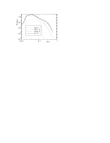
FIG. 1.: Wave spectra at different times.

Even though it is not clear from the Log-Log representation in Fig. 1, there is a downshifting of the peak of the spectrum towards lower wave numbers; as a consequences the steepness subsequently decreases over time. The time scale of the nonlinear energy transfer becomes larger and larger. In Fig 2 we show the power spectrum of the surface elevation after 4 hours (the steepnes of the wave field is $\varepsilon\simeq 0.07$). In the same plot we show two power laws $\sim k^{-2.5}$ and $\sim k^{-3}$: the first one seems to better fit the data. In order to be completely sure that the numerical data are in agreement with the prediction of Zakharov and Filonenko, we show in Fig. 3 compensated spectra with different compensation powers: $z=2.5$ seems to be the most plausible power law. Thus there seems to be ample evidence from our numerical simulations that the power law is in sufficiently good agreement with the value predicted by the theory.

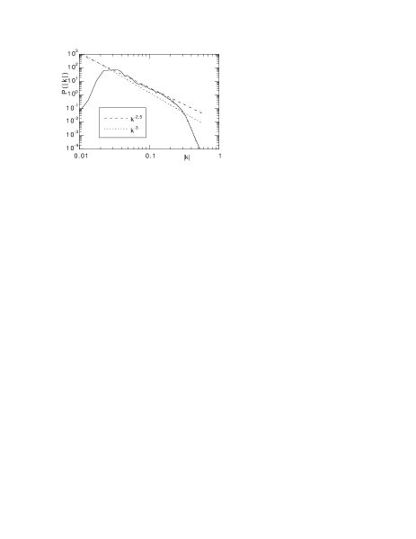
FIG. 2.: Wave spectrum at $t=4$ hours. A $k^{-2.5}$ (dotted-line) and a $k^{-3}$ (dashed-line) power law are also plotted.

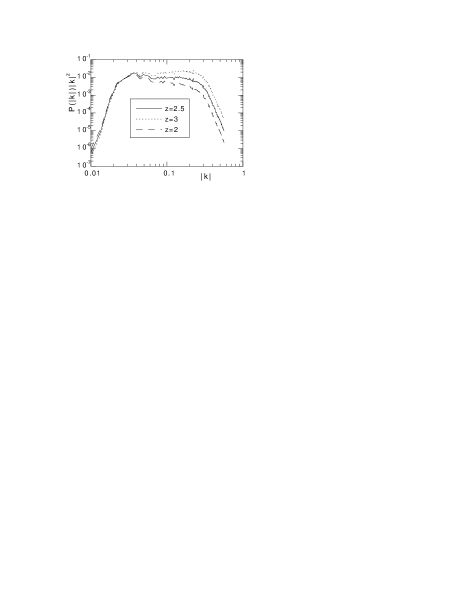
FIG. 3.: Compensated wave spectra for different values of the compensation power: $z=2$ (dahsed-line) $z=2.5$ (solid-line) and $z=3$ (dotted-line).

After the pioneering work by Zakharov and Filonenko the kinetic wave theory has developed further, making available quantitative predictions for other physical observables such as energy fluxes, downshifting of the peak, energy dissipation etc. All these quantities will be examined and results will be reported in future papers. Other questions naturally arise from our results: in HOS simulations the order of the computation depends on how many terms are retained in the Taylor expansion; do higher order terms influence the cascade process? Our computation has been performed in a freely decaying case; could external forcing (especially if anisotropic) influence the power law? And more, what would be the influence of the water depth? These are all questions to be answered in the near future.

Acknowledgements This work was supported by the Office of Naval Research of the United States of America (T. F. Swean, Jr.) and by the U.S. Army Engineer Research and Development Center. Consortium funds and Torino University funds (60 %) are also acknowledged. M. O. was also supported by a Research Contract from the Università di Torino.

REFERENCES

- [1] A. Kolmogorov, C. R. Akad. Sci. SSSR 30, 301 (1941).
- [2] O. M. Phillips, J. Fluid Mech 107, 426 (1958).
- [3] V.E. Zakharov and N. Filonenko, Soviet Phys. Dokl., 11, 881 (1967).
- [4] V.E. Zakharov, J. Appl. Mech. Tech. Phys. 9, 190 (1968).
- [5] V.E. Zakharov, G.Falkovich and V. Lvov, Kolmogorov spectra of turbulence I (Springer, Berlin, 1992).
- [6] Y. Toba, J. Phys. Ocean., 29, 209 (1973).
- [7] K. K. Kahama, J. Phys. Ocean. 11, 1503 (1981).
- [8] G. Z. Forristall, J. Geophys. Res. 86, 8075 (1981).
- [9] M. A. Donelan, J. Hamilton and W. H. Hui, Phil. Trans. R. Soc. Lond. A 315, 509 (1985).
- [10] O.M. Phillips, J. Fluid Mech. 156, 505, (1985).
- [11] D. Resio and W. Perrie, J. Fluid. Mech 223, 603 (1991).
- [12] A. Pushkarev, D. Resio and V. Zakharov, submitted to Phys. Rev. E (2001).
- [13] V. E. Zakharov, Eur. J. Mech. B-Fluid 18 327, (1999).
- [14] A. N. Pushkarev and V. E. Zakharov, Phys. Rev. Lett. 76, 3322, (1996).
- [15] D Cai, A. J. Majda, D. W. McLaughlin and E.G. Tabak, Physica D 152, 551, (2001).
- [16] V. E. Zakharov, P. Guyenne, A. N. Pushkarev and F. Dias, Physica D 152, 573, (2001).
- [17] W. T. Tsai, D.K.P. Yue, Ann. Rev. Fluid Mech. 28, 249, (1996).
- [18] B. J. West, K. A. Brueckner and R. Janda, J. Geophys. Res. 92, 11803, (1987).
- [19] D.G. Dommermuth and D.K.P. Yue, J. Fluid Mech. 184, 267 (1987).
- [20] M. Tanaka, J. Fluid Mech. 442, 303 (2001).
- [21] S. Yu. Annenkov and V.I. Shrira, J. Fluid Mech. 449, 341 (2001).
- [22] D. Clamond and J. Grue, J. Fluid Mech. 447, 337 (2001).
- [23] V. Zakharov, A. Dyachenko and O. Vasilyev, “New method for numerical simulation of a nonstationary potential flow of incompressible fluid with a free surface,” submitted for pubblication (2001).
- [24] J. Willemsen, Communication at the Theoretical developments: two and three dimensional water waves, EUConference, Cambridge, UK, August (2001).
- [25] V.P. Krasitskii, J. Fluid Mech. 272, 1 (1994).
- [26] G. Falkovich, Phys. of Fluids 6, 1411 (1994).
- [27] D. Biskamp, E. Schwarz, A. Celani, Phys.Rev. Lett. 81, 4855 (1998).
- [28] M. Onorato, A. R. Osborne and M. Serio, to be published in Phys. of Fluids, (2002).
- [29] A.N. Pushkarev and V. E. Zakharov, Physica D 135, 98 (2000).
- [30] L. E. Borgman, “Techniques for Computer Simulation of Ocean Waves”, in Topiccs in Ocean Physics, Proc. of the Int. School E. Fermi, Eds. A. R. Osborne and P. Malanotte Rizzoli, 373 (1980).