Thin front propagation in steady and unsteady cellular flows

Abstract

Front propagation in two dimensional steady and unsteady cellular flows is investigated in the limit of very fast reaction and sharp front, i.e., in the geometrical optics limit. In the steady case, by means of a simplified model, we provide an analytical approximation for the front speed, $v_{\mbox{{f}}}$, as a function of the stirring intensity, $U$, in good agreement with the numerical results and, for large $U$, the behavior $v_{\mbox{{f}}}\sim U/\log(U)$ is predicted. The large scale of the velocity field mainly rules the front speed behavior even in the presence of smaller scales. In the unsteady (time-periodic) case, the front speed displays a phase-locking on the flow frequency and, albeit the Lagrangian dynamics is chaotic, chaos in front dynamics only survives for a transient. Asymptotically the front evolves periodically and chaos manifests only in the spatially wrinkled structure of the front.

I Introduction

Front propagation in fluid flows is relevant to many fields of sciences and technology ranging from marine ecology [1, 2] to chemistry [3, 4] and combustion technology [5]. A complete description of the problem would require to consider the coupled evolution of reactants and velocity field, including the modification of the advecting field induced by the reaction. In general, this is a very difficult task [6]. Here we consider a simplified, but still physically significant, problem by neglecting the influence of the reactants on the velocity field. This amounts to consider the reaction as a constant-density process. Aqueous auto-catalytic reactions, and gaseous combustion with a large flow intensity but sufficiently low values of gas expansion across the flame are important examples of chemical-physical systems for which this approximations is appropriate [7].

In the simplest model a scalar field, $\theta({\bf r},t)$, which represents the fractional concentrations of the reaction’s products (i.e., $\theta=1$ indicates inert material, $\theta=0$ fresh one and $0<\theta<1$ means that fresh material coexists with products), evolves according to the advection-reaction-diffusion equation [8, 9]:

$$\partial_{t}\theta+{\bf u}\cdot{\boldmath{{\mbox{$\nabla$}}}}\theta=D_{0}\Delta\theta+{1\over\tau}f(\theta)\;,$$ (1)

where $D_{0}$ is the molecular diffusivity, and ${\bf u}$ is a given incompressible (${\boldmath{{\mbox{$\nabla$}}}}\cdot{\bf u}=0$) velocity field. $f(\theta)$ is the production term and $\tau$ its time scale.

Two limiting cases of Eq. (1) have been previously studied in detail: $f(\theta)\equiv 0$ and ${\bf u}\equiv{\bf 0}$. In the former, the equation for a passive scalar is recovered (for a review see Ref. [10]). The latter corresponds to the reaction-diffusion equation, which has gathered much attention since the seminal works of Fisher and Kolmogorov-Petrovsky-Piskunov (FKPP)[11, 12] (see also Ref. [9] and references therein).

Eq. (1) can be studied for different geometries and boundary conditions. For instance, one can consider an infinite strip in the horizontal direction with a reservoir of fresh material on the right and inert products on the left, and periodic boundary conditions along the transverse direction. With this geometry a front of inert material (stable phase) propagates from left to right. If the medium is at rest with the FKPP production term, $f(\theta)=\theta(1-\theta)$, the front propagates with an asymptotic speed and thickness given by [9, 11, 12]

$$v_{0}=2\sqrt{{D_{0}\over\tau}}\,,\qquad\xi=c\sqrt{{D_{0}\tau}}\,,$$ (2)

where $c$ is a constant depending on the definition adopted for $\xi$. This result is valid whenever $f(\theta)$ is a convex function ($f^{{}^{\prime\prime}}<0$) with $f(0)=f(1)=0$ and $f^{{}^{\prime}}(0)=1$. For non-convex $f(\theta)$ only upper and lower bounds for the front speed can be provided [9].

A more interesting physical situation is when the velocity field is non zero. In this case, generally, the front propagates with an average limiting speed, $v_{\mbox{f}}$, enhanced with respect to the fluid at rest ($v_{\mbox{f}}>v_{0}$). For very slow reaction, by means of homogenization techniques [10], one can show that the front speed behaves as in Eq. (2) with $D_{0}$ replaced by a renormalized diffusion coefficient, $D_{\mbox{{eff}}}$, the so-called eddy diffusivity (see Ref. [10] for an exhaustive review on the determination of the eddy-diffusivity). In realistic systems, the reaction time scale is of the same order or (more frequently) faster than the velocity time scale (fast reaction), so that a simple renormalization of $D_{0}$ is not sufficient to encompass the dynamical properties of the system [13]. In some cases the front speed can be still obtained by Eq. (2) renormalizing not only the diffusion constant, $D_{0}\to D_{\mbox{{eff}}}$, but also the reaction time $\tau\to\tau_{\mbox{{eff}}}$ [14]. However, a general method to compute $v_{\mbox{f}}$ for a generic velocity field does not exist.

Here we consider the limit of very fast reaction and very thin front, i.e., the so-called geometrical optics regime [7]. Formally, this corresponds to the limit $\tau\to 0$ and $D_{0}\to 0$ maintaining the ratio $D_{0}/\tau$ constant [15]: from (2) this means that $v_{0}$ is finite and $\xi\to 0$. In this regime the front is identified as a surface (a line in $2d$), and the effect of the velocity field is to wrinkle the front increasing its area (length in $2d$) and thereby its speed [8].

As to the velocity field we consider steady and unsteady cellular flows (i.e., with closed streamlines) in two-dimensions [16, 17, 18, 19]. Since coherent vortical structures are typically present in real hydrodynamical systems, cellular flows offer an idealized (but non-trivial) model to study the effects of this kind of structures on front propagation. Real flows, e.g., turbulent flows, are usually characterized by a very complex temporal dynamics and spatial development of scales. In this respect a steady cellular flow is too simple. Therefore, we also consider either the presence of small scale spatial structures in the velocity field, or the effects of time dependence, which induces a complex temporal behavior for particle trajectories –Lagrangian chaos [20, 21].

We found that the front speed is mainly determined by the large scales velocity characteristics, i.e., the effect of small scales is just to renormalize the largest scale velocity intensity. Concerning time periodic cellular flows, we found that the front speed is not significantly modified with respect to the steady case, although rather subtle effects appear. Namely the front speed locks on the flow frequency: a phenomenon which goes under the name of mode-locking (or frequency-locking) [22, 23], and which has been already found in some models of front propagation [24]. Lagrangian chaos is suppressed by the reaction and only survives for a transient. However, asymptotically the spatial wrinkling (“complexity”) of the front is enhanced with respect to the steady case. We introduced a suitable observable to quantify the front complexity.

The paper is organized as follows. In Section II we discuss the geometrical optics limit. Numerical results for steady cellular flows with one and more scales are presented in Section III, where we propose a simple model which well reproduces the numerical results. The effects of Lagrangian chaos and velocity phase-locking in time dependent cellular flows are discussed in Section IV. Final remarks are reported in Section V. The Appendices are devoted to the numerical methods here employed and to a more detailed treatment of the frequency-locking phenomenon.

II The geometrical optics limit

From a physical point of view the geometrical optics limit (in combustion jargon, the flamelet regime) corresponds to situations in which the reaction time scale and reaction zone thickness are much faster and much smaller than the time and length scales of the flow, respectively (e.g., in turbulent flows this means that the front thickness is smaller than the Kolmogorov length scale $\ell_{K}$, $\xi\ll\ell_{K}$) [8].

Being the front sharp, its dynamics can be described in terms of the evolution of the surface (line in $2d$) which divides the inert material ($\theta=1$) from the fresh one ($\theta=0$). In this limit the problem can be formulated in terms of the evolution of a scalar field, $G({\bf r},t)$, where the iso-line (in 2D) $G({\bf r},t)=0$ represents the front: $G>0$ is the inert material and $G<0$ is the fresh one. $G$ evolves according to the so-called $G$-equation [8, 15, 25, 26, 27, 28]

$${\partial G\over\partial t}+{\bf u}\cdot{\mbox{\boldmath$\nabla$}}G=v_{0}|{\mbox{\boldmath$\nabla$}}G|\,.$$ (3)

The analytical treatment of this problem is not trivial, and even in relatively simple cases (e.g., shear flows) numerical analysis is needed.

Recently Majda and collaborators [27] pointed out that there are situations in which the $G$-equation fails in reproducing the front speed of the original reaction-advection-diffusion model. Indeed, in some systems the exact treatment of Eq. (1) in the limit $\tau\to 0$, $D_{0}\to 0$ with $D_{0}/\tau=const$ does not lead to the same results of the $G$-equation. However, for the application we are interested in, the study of the $G$-equation is physically relevant [18].

In the absence of stirring (${\bf u}={\bf 0}$) the front evolves according to the Huygens principle, i.e., a point ${\bf x}$ belonging to the front surface moves with a velocity ${\bf v}({\bf x})=v_{0}\hat{\bf n}({\bf x})$, where $\hat{\bf n}({\bf x})$ is the perpendicular direction to the front surface in ${\bf x}$. With open boundary conditions, at large times the front surface is asymptotically close to a sphere (circle in $2d$). However, the preasymptotic behavior is mathematically non trivial [29] and interesting in some technological problems.

In the presence of stirring (${\bf u}\neq{\bf 0}$) the problem is much more difficult. The first attempt to determine the front speed in such a regime dates back to the $40$’s with the work of Damköler [8] who suggested that, if the velocity field does not change the local (bare) front speed, $v_{0}$, then the effective front speed is proportional to the total front area divided by the cross-section flow area. In two-dimensional geometry this means that

$$v_{\mbox{f}}/v_{0}=L_{\mbox{f}}/L$$ (4)

where $L$ is the transverse length, $v_{\mbox{f}}$ and $L_{\mbox{f}}$ are the average front speed and length respectively.

The average velocity and length are $v_{\mbox{{f}}}=\langle v(t)\rangle$ and $L_{\mbox{{f}}}=\langle{\cal L}(t)\rangle$, where $\langle\cdot\rangle$ indicates a time average. The instantaneous front velocity, $v(t)$, and length, ${\cal L}(t)$, can be defined as follows. The velocity is given by [16]

$$v(t)=\partial_{t}\left({1\over L}\int_{0}^{L}\!{\rm d}y\int_{-\infty}^{\infty}\!{\rm d}x\,\theta(x,y;t)\right)\,\,.$$ (5)

In order to define the instantaneous front length, ${\cal L}(t)$, we introduce the variable $\sigma_{\epsilon}(x,y;t)$ which assumes the value $0$ if $\theta$ is constant inside a circle of radius $\epsilon$ centered in $(x,y)$, otherwise $\sigma_{\epsilon}(x,y;t)=1$ (i.e., $\sigma_{\epsilon}(x,y;t)=1$ only if the $\epsilon$-ball centered in $(x,y)$ contains a portion of the front). The front length is then defined by

$${\cal L}(t)=\lim_{\epsilon\to 0}{1\over\epsilon}\int_{-\infty}^{\infty}{\rm d}x\,\int_{0}^{L}{\rm d}y\,\sigma_{\epsilon}(x,y;t)\,\,.$$ (6)

III Stationary Cellular Flow

We consider the following two-dimensional cellular flow, originally introduced in Ref. [30] to mimic roll patterns in Rayleigh-Bérnard convection,

$$\left\{\begin{array}[]{cc}u_{x}(x,y)=\!\!&U\sin\left({2\pi\over L}x\right)\cos\left({2\pi\over L}y\right)\\ \\ u_{y}(x,y)=\!\!&-U\cos\left({2\pi\over L}x\right)\sin\left({2\pi\over L}y\right)\,,\end{array}\right.$$ (7)

where $U$ is the flow intensity, $L$ the roll size (in the following for simplicity, $L=2\pi$). Periodic boundary conditions in the transverse directions are assumed. By fixing $\theta=1$ for $x\to-\infty$ and $\theta=0$ for $x\to\infty$ the front propagates from left to right. It is natural to expect that the front speed can be expressed according to the following relation [7, 25, 26]

$$v_{\mbox{f}}=v_{0}\psi\left({U\over v_{0}}\right)\,.$$ (8)

Our aim is to investigate the dependence of $v_{\mbox{f}}$ on the flow intensity $U$.

FIG. 1.: Front speed as a function of time, measured in the standard way $v(t)$ (5) ($\Box$) and as $x_{M}(t)/t$ (9)(o). The straight line is the average front speed $v_{\mbox{f}}$. The system parameters are $U=4$, $v_{0}=1$ and $L=2\pi$.

Due to the spatial periodicity of the flow, after an initial transient, the front propagates periodically in time (with period $T$). In Fig. 1 a typical time series of the instantaneous velocity $v(t)$ is reported: peaks occur when the front length is maximal. The front speed can be defined as the average $v_{\mbox{f}}=\langle v(t)\rangle_{T}$ over a period. Since the interface is sharp, we can easily track the farther edge of the interface ($x_{M}(t),y_{M}(t)$), i.e., the rightmost point (in the $x$-direction) for which $\theta(x_{M},y_{M};t)=1$. Thus we can define a velocity

$$\tilde{v}_{\mbox{f}}=\lim_{t\to\infty}{x_{M}(t)\over t}\,,$$ (9)

which, since the front dynamics is periodic, is equivalent to the standard definition (5) (see Fig. 1).

In Fig. 2 we show some snapshots of the front at different times. It is possible to see cusps and pockets of unburnt material (white) left behind the front edge, as firstly noticed by Ashurst and Sivanshinsky [31]. At high field intensity a trail of pockets is formed.

We now revert to the behavior of $v_{\mbox{f}}$ as a function of $U$. As far as we know, apart from very simple shear flows (for which $\psi({\cal U})={\cal U}+1$) [32], there are no general methods to compute $\psi({\cal U})$ from first principles. For the cellular flow under investigation, by mapping the front dynamics onto a one dimensional problem, it is possible to obtain an approximate expression for $\psi$ in good agreement with numerical data.

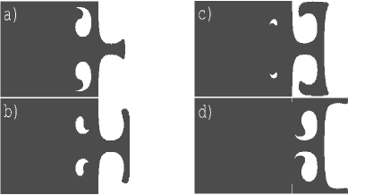
FIG. 2.: Snapshot of the front shape with time step $T/8$ (from (a) to (d)), where $T$ is the period of the front dynamics, for $v_{0}=0.5$, $U=4.0$ and $L=2\pi$.

The strategy is to devise an equation for the edge point evolution (shown in Fig. 3). After the transient, in the cell $[0,2\pi]\times[0,\pi]$, the point $(x_{M}(t),y_{M}(t))$ approximatively moves in the right direction along the separatrices, so that $y_{M}(t)$ practically assumes values close to $0$ or $\pi$. Therefore, one can reduce the edge dynamics to the following $1d$-problem

$${{\rm d}x_{M}\over{\rm d}t}=v_{0}+U\beta|\sin(x_{M})|\,.$$ (10)

The second term of the r.h.s. mimics the horizontal component of the velocity field, where $\beta$ takes into account the “average” effect of the dependence on the vertical coordinate, $y$. The periodicity of the r.h.s. of Eq. (10) implies that there exists a time $T_{M}$ such that $x_{M}(t+T_{M})=x_{M}(t)+\pi$. Then, by solving (10) in the interval $x_{M}\in[0,\pi]$ we computed $T_{M}$ and hence the front speed, $v_{\mbox{f}}=\pi/T_{M}$,

$$\psi_{\beta}({\cal U})={\pi{\sqrt{({\cal U}\beta)^{2}-1}}\over 2\ln\left({\cal U}\beta+\sqrt{({\cal U}\beta)^{2}-1}\right)}$$ (11)

Notice that (11) is valid only for ${\cal U}\beta\geq 1$, which is the regime we are interested in. Now the problem is to estimate $\beta$.

As stated previously the front evolution is periodic, so that $y_{M}(t)$ is a periodic function of time with period $T_{y}$ commensurate to $T_{M}$ (see Fig. 3); the front period $T$ should also be commensurable to $T_{M}$ and $T_{y}$. Therefore, for a specific value of $U$ and $v_{0}$ we numerically identified the period $T_{y}$ and computed $\beta$ as

$$\beta={1\over T_{y}}\int_{0}^{T_{y}}|\cos(y_{M}(t))|{\rm d}t\,,$$ (12)

obtaining $\beta\approx 0.875$. Using this value in (11) one has a remarkable agreement with the measured $v_{\mbox{f}}$, see Fig. 4 (the agreement is between $6\%$ and $10\%$ for all the range of investigated values of $U$ and $v_{0}$). Notice that, by definition, $\beta\!\leq\!1$. Therefore, with $\beta\!=\!1$ in Eq. (11) one obtains an upper bound for the front speed. Moreover, in Ref. [33], a rigorous lower bound has been provided:

$$v_{\mbox{f}}\geq U\,/\,\ln(1+U/v_{0})\,.$$ (13)

It is worth remarking that, for large $U$, both the upper and lower bounds give $v_{\mbox{f}}\sim\!U/\ln U$, which identify the asymptotic behaviour of the front speed.

FIG. 3.: Time evolution of the edge point: $x_{M}(t)$ and $y_{M}(t)$. The simulation parameters are the same of Fig. 1

Notwithstanding the considered cellular flow has only one spatial scale, it is interesting to compare the results with the relation [34]

$${v_{\mbox{f}}\over v_{0}}=\exp\left[d\left({U_{\mbox{{rms}}}\over v_{\mbox{f}}}\right)^{\alpha}\right]\,,$$ (14)

originally proposed by Yakhot [35] and Shivanshinsky [36] for (multi-scale) turbulent flows, where $U_{\mbox{{rms}}}$ is the turbulent intensity (i.e., the root mean square velocity) and $\alpha=2$ and $d=1$ are two parameters depending on the flow. Indeed, Eq. (14) has been frequently used in literature also for non turbulent flows and various values of $\alpha$ have been reported [7, 34]. In particular, for the same cellular flow here studied, Aldredge [25, 26] compared his numerical results with (14) for $\alpha=2$ and $d=1/\sqrt{2}$ finding a fairly good agreement (our data and Eq. (14) are shown in Fig. 4). Actually, the asymptotic behavior of Eq. (14) is $v_{\mbox{f}}\sim U/(\ln U)^{1/\alpha}$ which, by comparing with ours results, would suggest $\alpha=1$. In the following we investigate how small spatial scales modify the dependence of $v_{\mbox{{f}}}$ on the flow intensity.

FIG. 4.: The measured $v_{\mbox{{f}}}/v_{0}$ as a function of $U/v_{0}$ ($\Box$), data obtained using the measured values in Eq. (14) with $\alpha=2$ and $d=1/2$ (o) (see text), the function $\psi(U/v_{0})$ (11) for $\beta=0.875$ (solid line), and the upper and lower bounds, $\beta=1$ in Eq. (11) and Eq. (13), respectively (dotted lines).

A Effect of small scales

We consider now the following generalization of Eq. (7):

$$u_{x}( x,y)=U\sin\left(\frac{2\pi}{L}x\right)\cos\left(\frac{2\pi}{L}y\right)+$$ (16)

$$\sum_{n=1}^{N}Q_{n}\sin\left(\frac{2\pi}{L}k_{n}x+\phi^{x}_{n}\right)\cos\left(\frac{2\pi}{L}k_{n}y+\phi^{y}_{n}\right)$$

$$u_{x}( x,y)=-U\cos\left(\frac{2\pi}{L}x\right)\sin\left(\frac{2\pi}{L}y\right)-$$ (18)

$$\sum_{n=1}^{N}Q_{n}\cos\left(\frac{2\pi}{L}k_{n}x+\phi^{x}_{n}\right)\sin\left(\frac{2\pi}{L}k_{n}y+\phi^{y}_{n}\right)\,,$$

where $N$ is the number of different scales present in the flow, $\{k_{n}\}$ are integers giving the ratio between the different spatial scales, $Q_{n}$ is the velocity intensity at scale $\sim 1/k_{n}$, $\{\phi^{x}_{n}\,,\;\phi^{y}_{n}\}$ are (time-independent) phase differences.

In Fig. 5 we present two snapshots of the front for different parameters values. By comparing with Fig. 2 it is clear the presence of small structures in the front due to smaller scales in ${\bf u}$.

We computed $v_{\mbox{{f}}}$ for $N=1$ (two-scales flow) and $N=2$ (three-scales flow) with different values of $k_{n}$, $Q_{n}$ and random phases. In the case $N=2$, $Q_{n}=U\,k_{n}^{-1/3}$ has been chosen as a caricature of the power spectrum of three dimensional turbulence. The results, compared with the one-scale flow ($Q_{n}\!=\!0$) are summarized in Fig. 6, where $v_{\mbox{{f}}}$ is rescaled with $v_{0}$ and reported as a function of $U_{{\mbox{{rms}}}}/v_{0}$ ($U_{{\mbox{{rms}}}}\!=\!U\sqrt{(1+Q^{2}/U^{2})/2}$, with $Q^{2}\!=\!\sum_{n}Q_{n}^{2}$). As one can see, they roughly collapse onto a single curve together with the one scale results.

FIG. 5.: Images of the burnt area (black) for $U=6$, $Q=3$ (above) and $U=10$, $Q=2$ (below) with $k=5$, where $v_{0}=0.5$. The different scales are clearly visible.

The physical information one can extract from the above result is that the front speed is essentially determined by the large scale behavior of the velocity field (i.e., the flow intensity). Indeed, as previously observed [19] the absence of open channels can be more important than the detailed multi-scale properties of the flow.

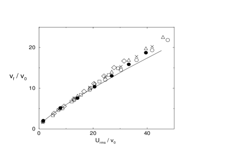
FIG. 6.: Front speeds $v_{\mbox{{f}}}/v_{0}$ as a function of $U_{{\mbox{{rms}}}}/v_{0}$ for the flow (18) for various $k_{n}$, $Q_{n}$-values and $v_{0}$ values. Filled line is the one scale data with $v_{0}=1.0$. Two scales data, with $v_{0}=0.5$, are: $Q_{1}=U/2$ and $k_{1}=3\,(\bigtriangleup)$, $Q_{1}=U/5$ and $k_{1}=3\,(\times)$, $Q_{1}=U/2$ and $k_{1}=5\,(\bullet)$, $Q_{1}=U/5$ and $k_{1}=5\,(\circ)$. For a turbulent caricature field we used $v_{0}=0.5$, $Q_{n}=Uk_{n}^{-1/3}$, $k_{n}=3^{n}$. The reported data refer to 2 scales ($\Box$) and 3 scales ($\Diamond$), only.

Let us conclude this section with some remarks. For the one scale flow in the steady case, we found that $v_{\mbox{{f}}}\sim U/\ln U$ as the flow intensity $U$ (or $U_{{\mbox{{rms}}}}$ equivalently) is very large. This corresponds to the large $U$ limit of the Yakhot like formula (14) with $\alpha=1$. Our results indicate that the main effect of the small scales is to renormalize the stirring intensity. Indeed once taken into account $U_{{\mbox{{rms}}}}$ all the curves roughly collapse (Fig. 6).

However, because of the limited range of spatial scales here investigated it is difficult to say something definitive on the front propagation in a multi-scale velocity field.

From Fig.s 5 and 6 one can see that the introduction of small scales on ${\mathbf{u}}$ causes a roughening of the front shape at the same scales of the velocity field, and has just a minor effect on the front speed. The problem of the effect of small scales on the front wrinkling has been studied also by Denet [37] in the context of the flame propagation equation (FPE) (which is similar to the Kardar Parisi Zhang equation [38]). In that model the small scales influence on the large scale motion seems to be important. However, it is not possible to make a direct comparison between the two results, because the FPE and Eq. (3) generate different dynamics.

IV Non-stationary cellular flow

We now consider the problem of front propagation in the time dependent cellular flow

$$\!\!\left\{\begin{array}[]{cc}\!u_{x}(x,y,t)=\!\!&\;\;U\sin\left[{2\pi\over L}x+B\sin(\omega t)\right]\cos\left[{2\pi\over L}y\right]\\ \\ \!\!u_{y}(x,y,t)=\!\!&-U\cos\left[{2\pi\over L}x+B\sin(\omega t)\right]\sin\left[{2\pi\over L}y\right]\end{array}\right.$$ (19)

where the term $B\sin(\omega t)$ mimics lateral oscillations of the roll pattern, which are produced by the oscillatory instability [30]. As one can see the steady case (7) corresponds to $B\!=\!\omega\!=\!0$. When $B,\omega\neq 0$ chaotic Lagrangian trajectories appear [20, 30]. The presence of complex particle trajectories constitutes a step toward more realistic flows.

We are mainly interested in addressing the two following issues. First, since trajectories starting near the roll separatrices typically have a positive Lyapunov exponent, it is natural to wonder about the role of Lagrangian chaos on front propagation. Second, from previous works [39, 40], we know that for the time dependent flow (19) the transport properties are strongly enhanced, therefore it is worth to see if similar effects are reflected also in the front speed.

A Effects of chaos: transient dynamics

A direct consequence of Lagrangian chaos is the exponential growth of passive scalar gradients and material lines [20, 21]: a (passive) material line of initial length $\ell_{0}$ for large times grows as

$$\ell(t)\sim\ell_{0}e^{\Lambda t}\,.$$ (20)

Where $\Lambda$ is the first generalized Lyapunov exponent,

$$\Lambda=\lim_{t\to\infty}\lim_{|\delta{\bf r}(0)|\to 0}{1\over t}\ln\left\langle{|\delta{\bf r}(t)|\over|\delta{\bf r}(0)|}\right\rangle\,,$$

which is in general larger than the maximum Lyapunov exponent [20, 21].

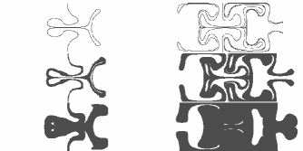
FIG. 7.: Snapshots at two successive times, $t=3.6$ and $7.5$, of the evolution of passive (top) and reactive line of material for two values of $v_{0}$ (middle $v_{0}=0.7$ and bottom $v_{0}=2.1$) for $U=1.9$, $B=1.1$ and $\omega=1.1U$. The initial condition is a straight vertical line.

The average in the previous equation is taken along the Lagrangian trajectories. In the presence of molecular diffusivity, the exponential growth of $\ell(t)$ stops due to diffusion [20] and chaos is just a transient [41].

FIG. 8.: ${\cal L}(t)/{\cal L}(0)$ as a function of time for $U\!=\!1.9$, $B\!=\!1.1$ and $\omega\!=\!1.1U$ for the passive ($+$) and reactive case: from top $v_{0}=0.3\,\,(\times),\,\;0.5\,\,(*),\,\;0.7\,\,(\Box)$. The straight line indicates the curve $\exp(\Lambda t)$ with $\Lambda\approx 0.5$, which has been directly measured.

For reacting scalars something very similar happens. Let us compare the evolution of material lines in the passive and reactive cases (see Fig. 7). While in the passive case structures on smaller and smaller scales develop (due to stretching and folding), in the reactive one after a number of folding events structures on smaller scales are inhibited as a consequence of the Huygens dynamics: the interface between the two phases merges. This phenomenon is responsible for the formation of pockets [25, 26, 31]. Of course, “merging” is more and more efficient as $v_{0}$ increases (compare the middle and lower pictures of Fig. 7).

In Fig. 8 we show the time evolution of the line length, ${\cal L}(t)$, as a function of $t$ for the passive and reactive material at different values of $v_{0}$. It is clear from the figure that while at small times both the passive and reactive scalar lines grow exponentially with a rate close to $\Lambda$, at large time $t>t^{*}$ (where $t^{*}$ is a transient time depending on $v_{0}$) the reacting ones stops due to merging. At stationarity, the front length varies periodically with an average value depending on $v_{0}$. A rough argument to estimate $t^{*}$, is the following: two initially separated part of the line (e.g., originally at distance $\ell_{0}$) become closer and closer, roughly as $\sim\ell_{0}\exp(-\Lambda t)$. When such a distance becomes of the order of $v_{0}t$ the merging takes place, hence to leading order

$$t^{*}\propto\frac{1}{\Lambda}\ln\left({\Lambda\ell_{o}\over v_{0}}\right)\,.$$ (21)

In the asymptotic state ($t>t^{*}$) both the spatial and temporal structures of the flow become periodic.

B Effects of chaos: asymptotic dynamics

Let us now switch to the effects of Lagrangian chaos on the asymptotic dynamics of front propagation. An immediate consequence of Eq. (21) is that the asymptotic front length (6) behaves as $L_{\mbox{f}}\sim v_{0}^{-1}$ for enough small values of $v_{0}$. Indeed,

$$L_{\mbox{f}}\sim Le^{\Lambda t^{*}}\sim\frac{L^{2}\Lambda}{v_{0}}\,\,,$$ (22)

which is in fairly good agreement with the simulations (see Fig. 9). It is interesting to note that in the steady case a different scaling can be seen. For the sake of completeness, in the inset of Fig. 9 we display the dependence of the front speed on $v_{0}$ for both the time-dependent and time-independent flow. For very small $v_{0}$, when chaos is effective in enhancing the front length, one observe an increasing of the front speed. At large values of $v_{0}$ the time-independent flow has a larger front speed than the time-dependent one. As we will see in the next subsection, this is a consequence of the mode-locking of the dynamics, which maintains constant the value of $v_{\mbox{f}}$.

It is worth remarking that even if the scaling (22) holds when chaos is present, in general it is not peculiar of chaotic flows. For instance, for the shear flow ($u_{x}=U\sin(y)\,,\;u_{y}=0$) one has $v_{\mbox{f}}=U+v_{0}$. On the other hand from Eq. (4) $v_{\mbox{f}}\sim L_{\mbox{f}}v_{0}$. Therefore, even if the shear flow is not chaotic $L_{\mbox{f}}\sim 1/v_{0}$ for $U/v_{0}\gg 1$. From the previous discussion, it seems that the front length dependence on $v_{0}$ is not an unambiguous effect of chaos on the asymptotic dynamics. But, comparing Fig. 2 with Fig. 7 appears that the spatial “complexity” of the front in the presence of Lagrangian chaos is higher than in its absence.

FIG. 9.: The average front length $L_{\mbox{f}}$ as a function of $v_{0}$ for the time dependent flow $(\circ)$, with $U=1.9$, $B=1.1$, $\omega=1.1U$ and the time independent case $(\times)$ with $U=1.9$. The straight line indicates the $1/v_{0}$ behavior. In the inset it is displayed $v_{\mbox{f}}$ versus $v_{0}$ for the time dependent $(\Box)$ and for the time independent case.

FIG. 10.: $L_{\mbox{f}}/W_{\mbox{f}}$ as a function of $v_{0}$ for the time dependent $(\circ)$ and independent $(\times)$ cases for the same parameters of Fig. 9.

In the sequel we introduce an indicator to quantitatively evaluate this qualitative observation.

Let us call $W_{\mbox{f}}$ the size of the region in which burnt and unburnt material coexist. Introducing a measure, $\mu(x)$, in that region we can defined $W_{\mbox{f}}$ as the standard deviation of $\mu(x)$ [24]:

$$\mu(x)={|\partial_{x}\tilde{\theta}(x)|\over\int{\rm d}x|\partial_{x}\tilde{\theta}(x)|}\,,$$ (23)

where $\tilde{\theta}(x)={1/L}\int_{0}^{L}\theta(x,y){\rm d}y$, i.e.,

$$W_{\mbox{f}}=\left(\int x^{2}\mu(x){\rm d}x-(\int x\mu(x){\rm d}x)^{2}\right)^{1/2}\,.$$ (24)

For a simple shear flow $W_{\mbox{f}}$ and $L_{\mbox{f}}$ display the same kind of dependence on $v_{0}$ (actually they are proportional). In generic chaotic flows there is an increasing of the front length, while chaotic mixing induces a decrease of $W_{\mbox{f}}$. This is indeed what one observes in Fig. 10, where we show the ratio $L_{\mbox{f}}/W_{\mbox{f}}$ both for the non-chaotic and the chaotic flow. For the latter this ratio diverges for very small $v_{0}$ values as a signature of chaos. From a physical point of view the ratio $L_{\mbox{{f}}}/W_{\mbox{{f}}}$ is an indicator of the spatial complexity of the front. Indeed it indicates the degree of wrinkling of the front with respect to the size of the region in which the front is present. Loosely speaking, we can say that the temporal complexity of Lagrangian trajectories converts in the spatial complexity of the front.

C Front speed dependence on the frequency

For passive particles transport in the flow (19), it has been found that the eddy diffusivity coefficient $D_{\mbox{{eff}}}(\omega)$ displays a complex behavior with resonant-like patterns [39, 40], in which the values of $D_{\mbox{{eff}}}(\omega)$ are orders of magnitude larger than the stationary-flow value, $D_{\mbox{{eff}}}(0)$. The physical mechanism responsible for the resonances is related to the interplay between the oscillation of the separatrices and the circulation inside the cell. When circulation and oscillation “synchronize”, a very efficient and coherent way of transferring particles from one cell to the other takes place. Does it happen something similar to the front speed in the reactive case? In Fig. 11 we report $v_{\mbox{f}}(\epsilon)$ as a function of $\epsilon=\omega/U$. As one can see, $v_{\mbox{f}}(\epsilon)$ varies both above and below the time independent value, $v_{\mbox{f}}(0)$, and its range of variability (about $30\%$ above or below the time independent value $v_{\mbox{f}}(0)$) is very small compared with that of the diffusion coefficient. This can be understood as a consequence of the inequality $v_{\mbox{f}}\leq U+v_{0}$. If one changes the value of $v_{0}$ then the curve display a small shift up (increasing $v_{0}$) or down (decreasing $v_{0}$) with some slight variations of the values of the peaks. This behavior is very robust with respect to changes of the flow parameters ($U$ and $B$). Moreover, $v_{\mbox{f}}(\epsilon)$ is a piece-wise linear function of $\epsilon$ with slope given by $U$ multiplied by a rational number. This phenomenon –called frequency locking [22, 23]– naturally arises in some non linear oscillators which are periodically forced, when the oscillator synchronizes its frequency to the one of the periodic forcing.

The frequency locking of the front speed can be understood with the following argument. At large times, $t>t^{*}$, the front is time and space periodic. This means that after a time period $T$, the front is rigidly translated in the $x$-direction by $S$, which is the spatial period. Due to the spatial periodicity of the flow (19) $S=2\pi N$ (where $N$ integer). Now, as confirmed by the simulations, one expects $T$ to be a multiple of the oscillation period $T_{o}=2\pi/\omega$ so that: $T=MT_{o}$ (with $M$ integer). On the other hand, the front speed is nothing but $S/T$ so that

$$v_{\mbox{f}}={S\over T}={2\pi N\over MT_{o}}={N\over M}\omega={N\over M}U\epsilon\,,$$ (25)

which is indeed the behavior we observed in Fig. 11.

FIG. 11.: $v_{\mbox{f}}(\epsilon)$ as a function of $\epsilon=\omega/U$, for the flow (19) with $U\!=\!1.9$, $v_{0}\!=\!0.2$ and $B\!=\!1.1$. The straight horizontal line indicates the front speed for the steady case, $B\!=\!0$. The dashed lines indicates the curves $U\epsilon N/M$ for different $(N,M)$ integers.

Varying $\omega$ the periods $S=2\pi M$ and $T=NT_{o}$ with a given $M$ and $N$ can loose their stability so that a new couple of $N,M$ values is selected. This explains the presence of different linear behaviors. By generalizing the one dimensional model (10) to the time dependent case one can qualitatively reproduce the behavior of the front speed dependence on the frequency (see Appendix B).

It is interesting to compare the behavior of front propagation with the time dependence (19) with previous studies that considered a different time dependence, i.e., with $U\rightarrow U\cos(\omega t)$ and $B=0$ in (19). With this choice the overall effect (as recognized by most of authors [31, 42] see also [43]) is a depletion of the front wrinkling at increasing the flow frequency. As a consequence, a strong bending of the front speed with respect to the steady case has been observed. This phenomenon has been quantitatively understood for the case of time dependent shear flows (i.e., ${\bf u}=(U\sin(\omega t)\sin(y),0)$) by Majda and collaborators [32]. With the choice (19) such a depletion is not observed because of the enhanced transport properties of the flow Fig. 11).

V Final remarks

In this paper we studied thin front propagation in steady and unsteady cellular flows. In particular, we investigated the behavior of the front speed and the front spatial structure at varying the system parameters.

As far as the one-scale steady case is concerned, we were able to give a quantitative description of the front speed by means of a simple one dimensional model. For large flow intensity $U$ (or $U_{\mbox{{rms}}}$ equivalently), the front speed behaves as $v_{\mbox{{f}}}\sim U_{\mbox{{rms}}}/\log(U_{\mbox{{rms}}})$, which corresponds to the asymptotic behavior of the Yakhot-like formula (14) with $\alpha=1$. Moreover, small scales structures have been added to the flow in order to study their effect on the front speed. Numerical simulations show that, once $v_{\mbox{{f}}}$ is rescaled with $v_{0}$ and reported as a function of $U_{{\mbox{{rms}}}}/v_{0}$, the results for the one-scale flow and those for more than one-scale fairly collapse onto a single curve. Therefore, the front speed is essentially determined by the large scale behavior of the velocity field.

Small scales spatial structures may also be induced by Lagrangian chaos. In this respect, on the basis of our results on the unsteady cellular flow it is interesting to remark that the effect of chaos is limited to a transient, in which the front behavior is close to the passive scalar case. Asymptotically, the reacting term induces a drastic regularization on the front evolution, suppressing the effects of small scales and Lagrangian chaos. Indeed the front propagates periodically and displays a frequency locking phenomenon.

The only asymptotic effect of Lagrangian chaos is in the structure of the front which is more and more wrinkled as $v_{0}$ approaches to zero. On the contrary in the case of steady velocity fields (regular Lagrangian motion) the degree of irregularity does not change with $v_{0}$. As an indicator of the spatial “complexity” of the front we used the ratio between the front length and the width, $L_{\mbox{{f}}}/W_{\mbox{{f}}}$ which is large (diverging as $v_{0}\to 0$) for the unsteady case and is roughly constant for the steady one.

VI Acknowledgments

We gratefully thank A. Malagoli and A. Celani for discussions and correspondences. This work has been partially supported by the INFM Parallel Computing Initiative and MURST (Cofinanziamento Fisica Statistica e Teoria della Materia Condensata). M.C., D.V. and A.V. acknowledge support from the INFM Center for Statistical Mechanics and Complexity (SMC).

A Numerical algorithm

In numerical approaches one is forced to discretize both space and time. We introduce a lattice of mesh size $\Delta x$ and $\Delta y$ (where we assume $\Delta x=\Delta y$) so that the scalar field is defined on the points ${\mathbf{x}}_{n,m}=(n\Delta x,m\Delta y)$: $\theta_{n,m}(t)=\theta(n\Delta x,m\Delta y,t)$.
The time discretization implies a discretization of the dynamics. Looking at the G-equation (3) one immediately recognize two different terms: the advection term ${\bf u}\cdot{\mbox{\boldmath$\nabla$}}G$, accounting for the transport properties of the flow, and the “optical” term $v_{0}|{\mbox{\boldmath$\nabla$}}G|$, which locally propagates the front in a direction perpendicular to it with a bare velocity $v_{0}$.

Let us call ${\mathbf{F}}^{\Delta t}$ the Lagrangian propagator for the discretized advection equation, $\partial_{t}{\bf x}={\bf u}\cdot{\mbox{\boldmath$\nabla$}}G$. Then, given the field at time $t$ one can computes the field at time $t+\Delta t$ using a two steps algorithm:

• using the Lagrangian propagator, ${\mathbf{F}}^{\Delta t}({\bf x})$, one evolves each point of the interface between burnt and unburnt region;

• at each point of the evolved interface one constructs a circle of radius $v_{0}\,{\rm\Delta}t$, obtaining the new frontier as the envelope of the circles.

FIG. 12.: Pictorial scheme of the numerical algorithm for the geometrical optics limit.

The numerical algorithm can be easily implemented using a time reversal procedure: starting on a grid point, ${\bf x}_{n,m}$, of the scalar field at time $t+\Delta t$ one applies the backward evolution obtaining the point ${\bf y}={\mathbf{F}}^{-\Delta t}{\bf x}_{n,m}$ at time $t$. Around $y$ we construct the circle of radius $v_{0}\,{\rm\Delta}t$. If in this circle there is at least one burnt point of the scalar field at time $t$, we fix $\theta({\bf x}_{n,m};t+{\rm\Delta}t)=1$ otherwise $\theta({\bf x}_{n,m};t+{\rm\Delta}t)=0$.

It is worth to note that one has to care about the radius of circle $v_{0}\,{\rm\Delta}t$ that has to be larger than the grid-size $\Delta x$ (empirically we found that $v_{0}\Delta t\geq 3-4\Delta x$ it is enough to give good results).

Typical values used in our simulation are $\Delta t=0.02$, $\Delta x=2\pi/2048$. The backward Lagrangian integration ${\mathbf{F}}^{-\Delta t}({\bf x})$ has been performed with a $4$-th order Runge-Kutta algorithm.

B Front speed locking

Frequency Locking arises in many physical systems ranging from Josephson-junction arrays to chemical reactions and non linear oscillators [22, 23, 24]. The basic mechanism is a resonance effect between two oscillators or when an oscillator is coupled with an external periodic forcing. In the last case the system synchronizes with the external forcing making its internal frequency commensurable with the external one. Almost all the systems displaying frequency locking can be mapped to the damped forced non linear oscillators [22]:

$$\alpha{d^{2}{\theta}\over dt^{2}}+\beta{d{\theta}\over dt}+\gamma\sin(\theta)=\delta+\sigma\cos(\omega t)\,.$$ (B1)

The solution $\theta(t)$ is periodic and the frequency, i.e., the average angular velocity, turns out to be:

$$\langle{d{\theta}\over dt}\rangle=\lim_{t\to\infty}{\theta\over t}={M\over N}\omega$$ (B2)

with $M,N$ integers. Moreover, if (B2) is realized for a certain set of the parameters there always exist an entire interval around their values where (B2) holds with the same values of $M$ and $N$. This kind of behavior persists also when $\alpha=0$ and for other kind of non linear terms (i.e., the third term of the l.h.s.). An exhaustive description of such a phenomenon can be found in Refs. [23].

FIG. 13.: $v_{M}(\epsilon)$ ad a function of $\epsilon=\omega/U$, for the model (B3) with $U=1.9$, $v_{0}=0.2$ and $B=1.1$. The dashed lines indicates the curves $U\epsilon N/M$ for different $N,M$ integers.

Coming back to our system, we can generalize the $1d$-model (10) to the time dependent case:

$${{\rm d}x_{M}(t)\over{\rm d}t}=v_{0}+U|\sin(x_{M}+B\sin(\omega t))|\,.$$ (B3)

Note that in principle one should also take into account the dynamics of $y_{M}$, but for the sake of simplicity we present just the $y$-independent version of the model. This model, although very idealized, is able to reproduce behaviors qualitatively similar to the ones observed in the simulations (compare Fig. 13) with Fig. 11). By changing of variables $z(t)=x_{M}(t)+B\sin(\omega t)$ Eq. (B3) reduces to

$${{\rm d}z(t)\over{\rm d}t}=v_{0}+U|\sin(z))|+B\omega\cos(\omega t)\,.$$ (B4)

which corresponds to (B1) for $\alpha=0$, and for which frequency locking has been studied in details. It is interesting to quote a recent work [44] which has studied the problem of locking in a model very similar to (B4) but in presence of noise. They found that the locking phenomenon is rather robust under the effect of noise and, moreover, it gives rise to resonances in the diffusion coefficient. All these results are qualitatively very similar to the behavior of the system here studied.

REFERENCES

- [1] E. R. Abraham, “The generation of plankton patchiness by turbulent stirring”, Nature 391, 577 (1998).
- [2] E. R. Abraham, C. S Law, P. W. Boyd PW, S.J Lavender, M. T Maldonado and A. R. Bowie, “Importance of stirring in the development of an iron-fertilized phytoplankton bloom”, Nature 407, 727 (2000).
- [3] J. Ross, S. C. Müller, and C. Vidal, “Chemical waves”, Science 240, 460 (1988).
- [4] I. R. Epstein, “The consequences of imperfect mixing in auto-catalytic chemical and biological systems”, Nature 374, 231 (1995).
- [5] F. A. Williams, Combustion Theory (Benjamin-Cummings, Menlo Park 1985).
- [6] S Malham and J. Xin, “Global solutions to a reactive Boussinesq system with front data on an infinite domain” Comm. Math. Phys. 199, 287 (1998).
- [7] P. D. Ronney, “Some open issues in premixed turbulent combustion”, in Modeling in Combustion Science, pp. 3-22, Eds. J. Buckmaster and T. Takeno (Springer-Verlag Lecture Notes in Physics, 1994).
- [8] N. Peters, Turbulent combustion (Cambridge University Press, 2000).
- [9] J. Xin, “Front Propagation in Heterogeneous Media”, SIAM Review 42, 161 (2000).
- [10] A. J. Majda, and P. R. Kramer, “Simplified models for turbulent diffusion: Theory, numerical modeling and physical phenomena”, Phys. Rep. 314, 237 (1999).
- [11] A. N. Kolmogorov, I. G. Petrovskii, and N. S. Piskunov, “Study of the diffusion equation with growth of the quantity of matter and its application to a biology problem”, Moscow Univ. Bull. Math. 1, 1 (1937).
- [12] R. A. Fischer, “The Wave of Advance of Advantageous Genes”, Ann. Eugenics 7, 355 (1937).
- [13] A.C. Marti, F. Sagues and J.M. Sancho, “Front dynamics in turbulent media”, Phys. Fluids 9, 3851 (1997).
- [14] M. Abel, A. Celani, D. Vergni and A. Vulpiani, “Front propagation in laminar flows”, Phys. Rev. E 64, 046307 (2001).
- [15] A. R. Kerstein, W.T. Ashurst, F. A. Williams, “Field equation for interface propagation in an unsteady homogeneous flow field”, Phys. Rev. A 37, 2728 (1988).
- [16] P. Constantin, A. Kiselev, A. Oberman and L. Ryzhik, “Bulk Burning Rate in Passive - Reactive Diffusion”, Arch. Rational Mechanics 154, 53 (2000).
- [17] B. Audoly, H. Beresytcki and Y. Pomeau, “Réaction diffusion en écoulement stationnaire rapide”, C. R. Acad. Sci. 328, Série II b, 255 (2000).
- [18] A. Bourlioux and A.J. Majda, “An elementary model for the validation of flamelet approximations in non-premixed turbulent combustion” Comb. Th. and Model. 4, 189 (2000).
- [19] W.T. Ashurst, “Flame propagation through swirling eddies, a recursive pattern”, Comb. Sci. Tech. 92, 87 (1993).
- [20] J.M. Ottino, The kinematics of mixing: stretching, chaos and transport (Cambridge University Press, 1989).
- [21] A. Crisanti, M. Falcioni, G. Paladin and A. Vulpiani, “Lagrangian Chaos: Transport, Mixing and Diffusion in Fluids”, La Rivista del Nuovo Cimento 14, 1 (1991).
- [22] M.H. Jensen, P. Bak and T. Bohr, “Complete devil’s Staircase, Fractal Dimension, and Universality of Mode-Locking Structure in the Circle Map”, Phys.Rev.Lett. 50, 1637 (1983).
- [23] A. Pikovsky, M. Rosenblum, and J. Kurths, Synchronization: A Universal Concept in Nonlinear Sciences, (Cambridge University Press, 2001)
- [24] R. Carretero-Gonzalez, DK. Arrowsmith and F. Vivaldi, “Mode-locking in coupled map lattices” Physica D 103, 381 (1997).
- [25] R. C. Aldredge, “The Scalar-Field Front Propagation Equation and its Applications”, in Modeling in Combustion Science, pp. 23-35, Eds., J. Buckmaster and T. Takeno (Springer-Verlag Lecture Notes in Physics, 1994).
- [26] R. C. Aldredge, “Premixed Flame Propagation in a High-Intensity, Large-Scale Vortical Flow”, Comb. and Flame 106, 29 (1996).
- [27] P. F. Embid, A. J. Majda and P. E. Souganidis, “Comparison of turbulent flame speeds from complete averaging and the G-equation”, Phys. Fluids 7 (8), 2052 (1995).
- [28] R.M. McLaughlin and J. Zhu, “The effect of finite front thickness on the enhanced speed of propagation”, Comb. Sci. Tech. 129, 89 (1997).
- [29] D. Benedetto, E. Caglioti and R. Libero, “Non-trapping sets and Huygens principle” Rairo-Math Model Num, 33, 517 (1999).
- [30] T.H. Solomon and J.P. Gollub, “Chaotic particle transport in time-dependent Rayleigh-Bénard convection”, Phys. Rev. A 38, 6280 (1988).
- [31] W.T. Ashurst and G. I. Shivanshinsky, “On flame propagation through periodic flow fields”, Comb. Sci. Tech. 80, 159 (1991).
- [32] B. Khouider, A. Bourlioux and A.J. Majda, “Parameterizing the burning speed enhancement by small-scale periodic flows: I. Unsteady shears, flame residence time and bending”, Comb. Th. Model. 5 295 (2001).
- [33] A. Oberman, PhD Thesis Univ. of Chicago 2001.
- [34] A. R. Kerstein and W.T. Ashurst, “Propagating rate of growing interfaces in stirred fluids”, Phys. Rev. Lett. 68, 934 (1992).
- [35] V. Yakhot, “Propagation velocity of premixed turbulent flame”, Comb. Sci. Tech. 60, 191 (1988).
- [36] G.I. Shivanshinsky, “Cascade-renormalization theory of turbulent flame speed”, Comb. Sci. and Tech. 62, 77 (1988).
- [37] B. Denet, “Are small scales of turbulence able to wrinkle a premixed flame at large scale?”, Comb. Theory and Modeling 2, 167 (1998).
- [38] M. Kardar, G. Parisi, and Y.-C. Zhang, Phys. Rev. Lett. 56, 889 (1986).
- [39] P. Castiglione, A. Mazzino, P. Muratore-Ginanneschi, A. Vulpiani, “On strong anomalous diffusion”, Physica D, 134, 75 (1999).
- [40] T. Solomon, A. Lee, M. Fogleman, “Resonant flights and transient super-diffusion in a time-periodic, two-dimensional flow”, Physica D 157 40 (2001).
- [41] A.K. Pattanayak “Characterizing the metastable balance between chaos and diffusion”, Physica D, 148, 1 (2001).
- [42] B. Denet, “Possible role of temporal correlations in the bending of turbulent flame velocity”, Comb. Th. Model. 3, 585 (1999).
- [43] W.T. Ashurst, “Flow-frequency effect upon Huygens front propagation”, Comb. Th. Model. 4 99 (2000).
- [44] D. Reguera, P. Reimann, P. Hänggi and J.M. Rubì, “Interplay of frequency-synchronization with noise: current resonances, giant diffusion and diffusion-crests”, Europhys. Lett. 57, 644 (2002).