Phys. Rev. Lett. 89, 24501

Topological Shocks in Burgers Turbulence

Abstract

The dynamics of the multi-dimensional randomly forced Burgers equation is studied in the limit of vanishing viscosity. It is shown both theoretically and numerically that the shocks have a universal global structure which is determined by the topology of the configuration space. This structure is shown to be particularly rigid for the case of periodic boundary conditions.

The $d-$dimensional randomly forced Burgers equation

$$\partial_{t}{\bm{u}}+({\bm{u}}\cdot\nabla){\bm{u}}=\nu\nabla^{2}{\bm{u}}-\nabla F(\bm{x},t),$$ (1)

appears in a number of physical problems, ranging from the dynamics of interfaces and cosmology to hydrodynamics (see, e.g., Ref. houches for a review). In the context of fluid dynamics, the Burgers equation, frequently referred to as “Burgers turbulence”, is a simple model for analyzing the signature of singularities, mostly shock discontinuities, in the statistics of the velocity field (see, e.g., Refs. cy95 ; p95 ; ekms ; eve99 ; b01 ). The (statistical) steady-state theory for Burgers turbulence in the limit of vanishing viscosity ($\nu\to 0$) was developed for $d=1$ in the spatially periodic case ekms . The analysis of the Lagrangian dynamics led to the distinguishing of a particular trajectory, the global minimizer, corresponding to the unique fluid particle that is never absorbed by a shock. The counterpart to the global minimizer is a unique main shock, with which all other shocks are merging after a finite time and hence, in which all the matter gets concentrated. Here the goal is to show that these objects, extended to multi-dimensional situations, determine the global structure of the stationary solution. This structure is strongly connected with the topology of the configuration manifold defined by the boundary conditions. We show that in any dimension, a unique global minimizer exists, so that the shocks have either a local or a global topological nature. The global shocks, unavoidably present in Burgers dynamics, are called the topological shocks; they have a nontrivial structure for $d>1$. For simplicity, we mostly consider space-periodic forcing potentials for which the configuration manifold is the $d$-dimensional torus ${\mathbb{T}}^{d}$ ($1$-periodic boundary conditions), but most of our work can be extended to other types of boundary conditions and configuration spaces.

If the initial data is of gradient type, the velocity field preserves this property at any later time, so that ${\bm{u}}({\bm{x}},t)=-\nabla\psi({\bm{x}},t)$, where the velocity potential $\psi$ solves the Hamilton–Jacobi equation

$$\partial_{t}\psi-\frac{1}{2}\left|\nabla\psi\right|^{2}=\nu\nabla^{2}\psi+F({\bm{x}},t).$$ (2)

When the external potential $F$ is delta-correlated in both space and time, this equation is known as the Kardar–Parisi–Zhang model for interface dynamics kpz86 . We focus here on smooth-in-space forcing potentials with a correlation function given by

$$\left\langle F({\bm{x}}_{1},t_{1})F({\bm{x}}_{2},t_{2})\right\rangle=G({\bm{x}}_{1}-{\bm{x}}_{2})\,\delta(t_{1}-t_{2}),$$ (3)

where $G$ is a smooth large-scale function. This type of large-scale forcing was chosen analogous with that usually assumed in work on forced Navier–Stokes turbulence. Note that the results discussed in this Letter can be extended to other types of random forcing (e.g. with a finite correlation time). Because of space periodicity, the average velocity ${\bm{b}}\equiv\int_{{\mathbb{T}}^{d}}{\bm{u}}({\bm{x}},t)d{\bm{x}}$ is an integral of motion. Its value does not affect the structure of the topological shocks and, for simplicity, we choose $\bm{b}=0$.

The initial-value problem associated to the Hamilton–Jacobi equation (2), in the inviscid limit $\nu\to 0$, has a variational solution variational . Denoting $\psi_{0}$ the potential at the initial time $t_{0}$, the velocity potential at times $t>t_{0}$ is given by

$$\psi(\bm{x},t)=-\inf_{\bm{\gamma}(\cdot)}\left[{\cal A}(\bm{\gamma},t)-\psi_{0}(\bm{\gamma}(t_{0}))\right],$$ (4)

where the infimum is taken over all differentiable curves $\bm{\gamma}:[t_{0},t]\to{\mathbb{T}}^{d}$ such that $\bm{\gamma}(t)=\bm{x}$ and ${\cal A}$ is the Lagrangian action

$${\cal A}({\bm{\gamma}},t)\equiv\int_{t_{0}}^{t}\left(\frac{1}{2}\left|\dot{\bm{\gamma}}(\tau)\right|^{2}-F({\bm{\gamma}}(\tau),\tau)\right)d\tau.$$ (5)

A minimizing trajectory is called a minimizer on the interval $[t_{0},t]$ and is associated to a fluid particle reaching $\bm{x}$ at time $t$. In the limit $t_{0}\to-\infty$, a stationary regime is obtained, independent of $\psi_{0}$. The solution is then determined by one-sided minimizers, i.e. action-minimizing trajectories from $-\infty$ to $t$. It is easily seen from Eq. (4) that all the minimizers are solutions of the Euler–Lagrange equations

$$\dot{\bm{\gamma}}(\tau) = \bm{v}(\tau),$$ (6)

$$\dot{\bm{v}}(\tau) = -\nabla F(\bm{\gamma}(\tau),\tau).$$ (7)

A global minimizer (or a two-sided minimizer) is defined as a curve which minimizes the action for any time interval $[t_{1},t_{2}]$ and thus corresponds to the trajectory of a fluid particle that is never absorbed by shocks.

We now state three main results whose rigorous proof is given in Ref. ik01 and that are essential for the introduction of topological shocks. First, there exists a unique solution of the Hamilton–Jacobi equation (2) in the limit $\nu\to 0$ which is extendible to all times. This solution is continuous and almost everywhere differentiable in space. It generates uniquely a stationary distribution for the random Hamilton-Jacobi equation and its gradient defines a unique statistically stationary solution of the inviscid Burgers equation. Second, for a given time and for every space location where the potential is differentiable, there exists a unique one-sided minimizer. The locations where the one-sided minimizers are not unique correspond to shock positions. Finally, there exists a unique global minimizer. This third statement is crucial for the construction of topological shocks because it implies that for large negative times $\tau\to-\infty$, all the one-sided minimizers are asymptotic to the global minimizer remark2 .

To introduce the notion of topological shock, we “unwrap”, at a given time $t$, the configuration space ${\mathbb{T}}^{2}$ to the entire space ${\mathbb{R}}^{d}$ (see Fig. 1(a)). Now, for a given realization of the forcing, we obtain instead of a single global minimizer an infinite number of them, each being the image of others by integer shifts. They form a lattice parameterized by vectors $\bm{k}$ with integer components and are denoted $\bm{\gamma}^{(\rm g)}_{\bm{k}}$. The backward-in-time convergence to the global minimizer on ${\mathbb{T}}^{d}$ implies that every one-sided minimizer emanating from some location in ${\mathbb{R}}^{d}$ is asymptotic to a particular global minimizer $\bm{\gamma}^{(\rm g)}_{\bm{k}}$ on the lattice. Hence, every location $\bm{x}$ which has a unique one-sided minimizer is associated to an integer vector $\bm{k}(\bm{x})$, defining a tiling of the space at time $t$. The tiles $O_{\bm{k}}$ are the sets of points whose associated one-sided minimizer is asymptotic to the $\bm{k}$-th global minimizer. The boundaries of the $O_{\bm{k}}$’s correspond to the positions of particular shocks that are called the topological shocks. They are the locations for which at least two one-sided minimizers approach different global minimizers on the lattice. Indeed, a point where two tiles $O_{\bm{k}_{1}}$ and $O_{\bm{k}_{2}}$ meet, has at least two one-sided minimizers, one of which is asymptotic to $\bm{\gamma}^{(\rm g)}_{\bm{k}_{1}}$ and another to $\bm{\gamma}^{(\rm g)}_{\bm{k}_{2}}$. Of course, there are also points on the boundaries where three or more tiles meet and thus where more than two one-sided minimizers are asymptotic to different global minimizers. For $d=2$ such locations are isolated points corresponding to the intersections of three or more topological shock lines, while for $d=3$, they form edges and vertices where shock surfaces meet. Note that, generically, there exist other points inside $O_{\bm{k}}$ with several minimizers. They correspond to shocks of “local” nature because at these locations, all the one-sided minimizers are asymptotic to the same global minimizer $\bm{\gamma}^{(\rm g)}_{\bm{k}}$ and hence, to each other. In terms of mass dynamics, the topological shocks play a role dual to that of the global minimizer. Indeed, all the fluid particles are converging backward-in-time to the global minimizer and are absorbed forward-in-time by the topological shocks. Assuming that the Burgers equation (1) is accompanied by a continuity equation for the mass density, this implies that all the mass concentrate at large times in the topological shocks.

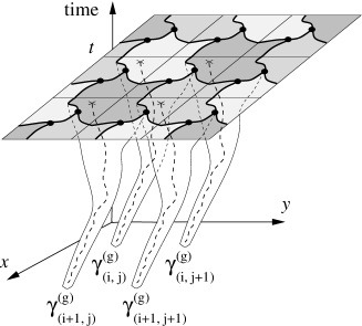
(a)

(b)

Figure 1: (a) Sketch in space-time of the unwrapped picture for $d=2$; on the horizontal plane which corresponds to a lattice of periodic box replicas at time $t$, the bold lines denote the topological shocks and triple points are represented by dots. The different “horns” illustrate the backward-in-time convergence to four different global minimizers represented as dashed lines and the filled areas represent different tiles $O_{\bm{k}}$. (b) Position of the topological shock on the torus; the two triple points are represented as dots.

We now describe the global structure of the topological shocks. Parameter counting suggests that there are generically $(d-1)$-dimensional surfaces of points with two one-sided minimizers which contain $(d-2)$-dimensional sub-manifolds with three one-sided minimizers and so on. This ends up with single points (zero-dimension) from which emanate $(d+1)$ one-sided minimizers. As one expects to see only generic behavior in a random situation, the probability to have points associated to more than $(d+1)$ one-sided minimizers is zero. It follows that there are no points where $(d+2)$ tiles $O_{\bm{k}}$ meet, an important restriction on the structure of the tiling. Thus for $d=2$, the tiling is constituted of curvilinear hexagons. Indeed, suppose each tile $O_{\bm{k}}$ is a curvilinear polygon with $s$ vertices corresponding to triple points. For a large piece of the tiling which consists of $N$ tiles, the total number of vertices is $n_{v}\sim sN/3$ and the total number of edges is $n_{e}\sim sN/2$. The Euler formula implies that $1=n_{v}-n_{e}+N\sim(6-s)N/6$; so we have $s=6$, corresponding to an hexagonal tiling. As shown in Fig. 1(b), this structure corresponds on the periodicity torus ${\mathbb{T}}^{2}$, to two triple points connected by three shock lines which are the curvilinear edges of the hexagon $O_{\bm{0}}$. The connection between the steady state velocity potential and the topological shocks is shown on Fig. 2 which was obtained numerically.

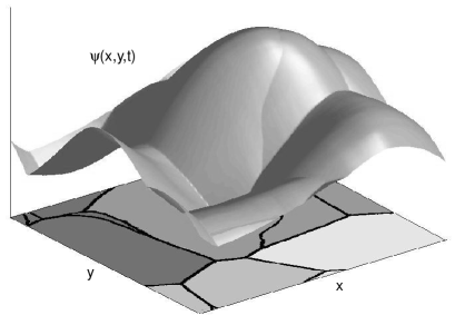
Figure 2: Snapshot of the velocity potential $\psi(x,y,t)$ for $d=2$ in the statistical steady state, obtained numerically with $256^{2}$ grid points. Shock lines, corresponding to locations where $\psi$ is not differentiable, are represented as black lines on the bottom of the picture; the four gray areas are different tiles separated by the topological shocks; the other lines are local shocks.

Although the topological shocks always form hexagonal patterns when $d=2$, the corresponding tilings can be of different types; in the course of time, the merger of two triple points is the generic mechanism for changing the type of the tiling. This so-called flipping bifurcation AppendixBookGurbatov has the property of redistributing matter among nodes, so that the mass does not concentrate in a particular triple point. In higher dimensions, the structure of topological shocks can be more complex; for instance, it is not possible to determine uniquely the shape of polyhedra forming the tiling. Nevertheless, the minimal polyhedra defining such tilings for $d=3$ can be shown to have 24 vertices anisov ; matveev .

All the above results concerning the global structure of solutions require a statistical steady state, achieved asymptotically at large times. The convergence to this regime is actually exponential so that, generally, the global picture of the flow is reached after just a few turnover times. The nature of the convergence is related to the local properties of the global minimizer and more particularly to its hyperbolicity. For $d=1$, the global minimizer has been shown to be a hyperbolic trajectory of the dynamical system defined by the Euler–Lagrange equations (6-7) ekms . In multi-dimensional situations the hyperbolicity of the global minimizer is an open problem. Since the Lagrangian flow defined by (6-7) is Hamiltonian, one can define $d$ pairs of non-random Lyapunov exponents with opposite signs. Hyperbolicity means that none of these exponents vanishes. This question can be addressed in terms of the backward-in-time convergence of the one-sided minimizers to the global one or, in terms of forward-in-time dynamics, by looking at how fast Lagrangian fluid particles are absorbed into shocks. For this, we consider the set $\Omega(T)$ of locations $\bm{x}$ such that the fluid particle at $\bm{x}$ at time $t=0$ survives, i.e. is not absorbed by any shock, until the time $t=T$. The long-time shrinking of $\Omega$ as a function of time is asymptotically governed by the Lyapunov exponents. To ensure the absence of vanishing Lyapunov exponents, it is sufficient to show that the diameter of $\Omega(T)$ decays exponentially as $T\to\infty$. Below we demonstrate numerically that this is indeed the case for $d=2$.

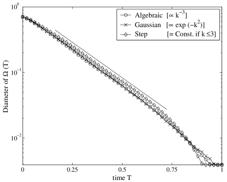
Figure 3: Time evolution of the diameter of the Lagrangian set $\Omega(T)$ (points corresponding to the regular region) for three different types of forcing spectra normalized to give the same Lyapunov exponents; average over 100 realizations and with $256^{2}$ grid points.

For this we assume that the forcing is a sum of independent random impulses concentrated at discrete times bfk00 , a case to which the present theory remains applicable. Between “kicks” the velocity field decays according to the unforced Burgers equation. This allows us to use the fast Legendre transform method nv94 , based on discrete approximations of the one-sided minimizers over a grid, which gives directly the solution in the inviscid limit and is particularly useful due to its strong connection with the Lagrangian picture of the flow. We can then track numerically the set $\Omega(T)$ of regular Lagrangian locations. As shown in Fig. 3 for three different types of forcings, the diameter of this set decays exponentially in time, providing strong evidence for the hyperbolicity of the global minimizer when $d=2$.

Since all the one-sided minimizers converge backward-in-time to the global minimizer, hyperbolicity implies that, in the statistical steady state, the graph of the solution in the phase space $({\bm{x}},{\bm{u}})$ is made of pieces of the smooth unstable manifold associated to the global minimizer with discontinuities along the shocks lines or surfaces. In other words, shocks appear as jumps between two different folds of the unstable manifold. The smoothness of the unstable manifold is key; for instance, it implies that when $d=2$, the topological shock lines are smooth curves. The above geometrical construction of the solution has much in common with that appearing in the unforced problem. Indeed, when $F=0$, the solution can be obtained by considering in the $({\bm{x}},{\bm{u}})$ space, the Lagrangian manifold defined by the position and the velocity of the fluid particles at a given time. This analogy gives good ground to conjecturing that several universal properties associated to the unforced problem still hold in the forced case, as indeed happens in one dimension ekms ; b01 . Hyperbolicity implies that there exists a strong parallel between the forced and the unforced situations. Despite the fact that the mass dynamics is completely different in the two cases (mass is absorbed by shocks linearly in time in the decaying case and exponentially fast in the forced case), many features of the velocity field are universal. For instance, it was shown in Ref. fbv01 that, for the unforced case and $d>1$, large but finite mass densities are localized near time-persistent boundaries of shocks (“kurtoparabolic” singularities) contributing, in any dimension, power-law tails with the exponent $-7/2$ in the probability density function (PDF) of both velocity gradients and mass densities. When a force is applied, the geometry of the solutions is very similar to that appearing in unforced situations. This leads again to a universal $-7/2$ power-law behavior of the PDF of velocity gradients and mass density, irrespective of $d$. The issue of similarities between forced and unforced Navier–Stokes turbulence and the search for universal statistical properties of the velocity field is, of course, still an open problem.

Note, finally, an important physical problem which will be addressed in a future work, namely the understanding of the behavior of minimizers and the effects related to global shocks in the case of spatially extended non-periodic systems. This amounts to investigating intermediate time asymptotics when the size of the system is much larger than the forcing scale. Preliminary numerical results indicate the appearance of a shock structure resembling the structure of topological shocks.

We are grateful to S. Anisov, I. Bogaevski, U. Frisch, T. Matsumoto, S. Novikov, Ya. Sinai, S. Tarasov for illuminating discussions and useful remarks. R.I. was supported by CONACYT-México grant 36496-E. Simulations were performed in the framework of the SIVAM project of the Observatoire de la Côte d’Azur, funded by CNRS and MENRT.

References

- (1) U. Frisch and J. Bec, “Burgulence”, in Les Houches 2000: New Trends in Turbulence, M. Lesieur, A. Yaglom and F. David eds. (Springer EDP-Sciences, 2001), p. 341; also http://xxx.arxiv.org/abs/nlin.CD/0012033
- (2) A. Chekhlov and V. Yakhot, Phys. Rev. E 51, R2739 (1995).
- (3) A. Polyakov, Phys. Rev. E 52, 6183 (1995).
- (4) W. E, K. Khanin, A. Mazel and Ya. Sinai, Phys. Rev. Lett. 78, 1904 (1997); Ann. Math. 151, 877 (2000).
- (5) W. E and E. Vanden Eijnden, Phys. Rev. Lett. 83, 2572 (1999); Comm. Pure Appl. Math. 53, 852 (2000).
- (6) J. Bec, Phys. Rev. Lett. 87, 104501 (2001).
- (7) M. Kardar, G. Parisi and Y.-C. Zhang, Phys. Rev. Lett. 56, 889 (1986).
- (8) P.D. Lax, Comm. Pure Appl. Math. 10, 537 (1957); O. Oleinik, Uspekhi Mat. Nauk 12, 3 (1957) [Am. Math. Transl. Series 2 26, 95]; P.-L. Lions, Generalized solutions of Hamilton-Jacobi equations, (Pitman Research Notes in Math. 69, Boston, 1982).
- (9) R. Iturriaga and K. Khanin, in Proceedings of the Third European Congress of Mathematics, Barcelona July 2000 (Progress in Mathematics, Birkhauser, Boston–Basel–Berlin, 2001); Burgers Turbulence and Random Lagrangian Systems, preprint (2001).
- (10) Although there are no doubts that backward-in-time convergence of one-sided minimizers to the global one always holds, we were able to prove it rigorously only for a non-random sequence of times . Notice, however, that convergence for a sequence is enough for the construction of the topological shocks.
- (11) V. Arnol’d, Yu. Baryshnikov and I. Bogaevski, in S. Gurbatov, A. Malakhov and A. Saichev, Non-linear random waves and turbulence in nondispersive media: waves, rays and particles (Manchester University Press, Manchester, 1991), p. 290.
- (12) S. Anisov, Upper bounds for the complexity of some 3-dimensional manifolds, Newton Institute preprint NI00037-SGT (2000).
- (13) S. Matveev, Acta Appl. Math. 19, 101 (1990); Tables of 3-manifolds up to complexity 6, Max Planck Institute preprint MPI1998-67 (1998).
- (14) J. Bec, U. Frisch and K. Khanin, J. Fluid Mech. 416, 239 (2000).
- (15) A. Noullez and M. Vergassola, J. Sci. Comput. 9, 259 (1994).
- (16) U. Frisch, J. Bec and B. Villone, Physica D 152–153, 620 (2001).