Intermittency in two-dimensional Ekman-Navier-Stokes turbulence

Abstract

We study the statistics of the vorticity field in two-dimensional Navier-Stokes turbulence with a linear Ekman friction. We show that the small-scale vorticity fluctuations are intermittent, as conjectured by Nam et al. [Phys. Rev. Lett. 84 (2000) 5134]. The small-scale statistics of vorticity fluctuations coincides with the one of a passive scalar with finite lifetime transported by the velocity field itself.

In many physical situations, the incompressible flow of a shallow layer of fluid can be described by the two-dimensional Navier-Stokes equations supplemented by a linear damping term which accounts for friction. An important example comes from geophysical rotating flows subject to Ekman friction [1]. The dynamics can be written in terms of a single scalar field, the vorticity $\omega={\mbox{\boldmath$\nabla$}}\times{\mbox{\boldmath$v$}}$, which obeys the equation

$${\partial\omega\over\partial t}+{\mbox{\boldmath$v$}}\cdot\nabla\omega=\nu\nabla^{2}\omega-\alpha\omega+f_{\omega}\;,$$ (1)

where $\nu$ is the fluid viscosity, and $\alpha$ is the Ekman friction coefficient. The term $f_{\omega}$ is an external source of energy – e.g. stirring – that counteracts the dissipation by viscosity and friction and allows to obtain a statistically steady state. Here, we will study the statistical properties of vorticity fluctuations $\delta_{r}\omega=\omega({\mbox{\boldmath$x$}}+{\mbox{\boldmath$r$}},t)-\omega({\mbox{\boldmath$x$}},t)$ at scales $r$ smaller than the correlation length $L$ of the external forcing. We will show that the statistics of $\delta_{r}\omega$ is intermittent, and that the vorticity field has the same scaling properties as a passive scalar with a finite lifetime.
As shown in Figure 1, the vorticity field resulting from the numerical integration of Eq. (1) is characterized by filamental structures whose thickness can be as small as the smallest active lengthscales. The wide range of scales involved in the vorticity dynamics manifests itself in the appearance of power-law scaling for the spectrum of vorticity fluctuations $Z(k)=2\pi k\langle|\hat{\omega}({\mbox{\boldmath$k$}})|^{2}\rangle\sim k^{-1-\xi}$. As already shown by Nam et al [2], the spectral slope $-1-\xi$ depends on the intensity of the Ekman drag: for the frictionless Navier-Stokes case ($\alpha=0$) we have $\xi=0$; a non-vanishing friction regularizes the flow depleting the formation of small-size structures and results in a steeper spectrum (see Fig. 2). In the range $0<\xi<2$ the exponent $\xi$ coincides with the scaling exponent $\zeta_{2}$ of the second-order moment of vorticity fluctuations $S^{\omega}_{2}(r)=\langle(\delta_{r}\omega)^{2}\rangle\sim r^{\zeta_{2}}$. Let us now focus on a given value of $\alpha$. In Figure 3 we show the probability density functions of vorticity fluctuations $\delta_{r}\omega$ at various $r$, rescaled by their rms value $\langle(\delta_{r}\omega)^{2}\rangle^{1/2}$. As the separation decreases, we observe that the probability of observing very weak or very intense vorticity excursions increases at the expense of fluctuations of average intensity. This phenomenon goes under the name of intermittency. Its visual counterpart is the organization of the field into “quiescent” areas (the patches, where vorticity changes smoothly) and “active” regions (the filaments, across which the vorticity experiences relatively strong excursions).

                          

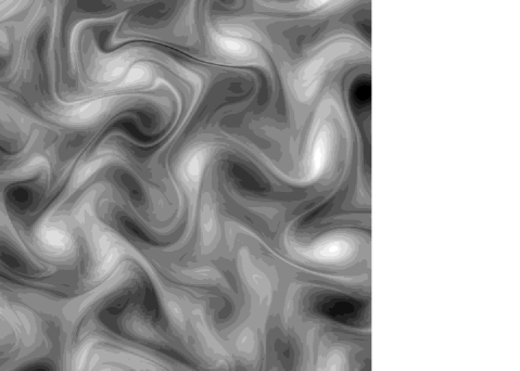
FIG. 1.: Snapshot of the vorticity field. The numerical integration of Eq. (1) is performed by a fully dealiased pseudospectral code with a second-order Runge-Kutta scheme, on a doubly periodic square domain of size $L=2\pi$ at different resolutions: $N^{2}=512^{2},1024^{2},2048^{2}$ grid points. (The present figure is taken from the $1024^{2}$ run). Standard viscosity or hyperviscosity (depending on the resolution) is used to remove the remnant enstrophy flux at small scales. The large-scale forcing $f_{\omega}$ is Gaussian, $\delta$-correlated in time, and limited to a shell of wavenumbers around $k_{f}=2\pi/L$ ($k_{f}=2$ for $N=512,2048$, and $k_{f}=8$ for $N=1024$). At variance with other choices for $f_{\omega}$ commonly used (e.g. large-scale shear) this kind of forcing ensures the statistical isotropy and homogeneity of the vorticity field.

The dynamical origin of this phenomenon can be understood as follows (see also Ref. [2]). Let us first notice that, for any $\alpha$ strictly positive and as far as the statistical properties in the scaling range are concerned, we can disregard the viscous term in Eq. (1). In other words, this system shows no dissipative anomaly, due to the presence of friction [3]. In the inviscid limit ($\nu=0$), Eq. (1) can be solved by the method of characteristics yielding the expression $\omega({\mbox{\boldmath$x$}},t)=\int_{-\infty}^{t}f_{\omega}({\mbox{\boldmath$X$}}(s),s)\,\exp[-\alpha(t-s)]\,ds$, where ${\mbox{\boldmath$X$}}(s)$ denotes the trajectory of a particle transported by the flow, $\dot{\mbox{\boldmath$X$}}(s)={\mbox{\boldmath$v$}}({\mbox{\boldmath$X$}}(s),s)$, ending at ${\mbox{\boldmath$X$}}(t)={\mbox{\boldmath$x$}}$. The uniqueness of the trajectory ${\mbox{\boldmath$X$}}(s)$ in the limit $\nu\to 0$ is ensured by the fact that the velocity field is Lipschitz-continuous, as it can be seen from the velocity spectrum $E(k)=Z(k)/k^{2}\sim k^{-3-\xi}$, always steeper than $k^{-3}$ (see Fig. 2). We remark that for $\xi>0$ the second-order velocity structure function is dominated by the IR contribution of the spectrum and thus trivially displays smooth scaling independently of the value of $\xi$. This is not the case for odd order structure functions that, in the absence of enstrophy dissipative anomaly, display anomalous scaling at the leading order [4]. We have checked that this is indeed the case in our simulations.

FIG. 2.: The vorticity spectrum $Z(k)\sim k^{-1-\xi}$ steepens by increasing the Ekman coefficient $\alpha$. Here $\alpha=0.15$ $(+)$, $\alpha=0.23$ $(\times)$, $\alpha=0.30$ $(\odot)$. In the inset, the exponent $\xi$ as a function of $\alpha$.

Vorticity differences are then associated to couples of particles $\omega({\mbox{\boldmath$x$}}^{\prime},t)-\omega({\mbox{\boldmath$x$}},t)=\int_{-\infty}^{t}[f_{\omega}({\mbox{\boldmath$X$}}^{\prime}(s),s)-f_{\omega}({\mbox{\boldmath$X$}}(s),s)]\exp[-\alpha(t-s)]\;ds$. Inside the time integral, the difference between the value of $f_{\omega}$ at ${\mbox{\boldmath$X$}}^{\prime}$ and that at $X$ is negligibly small as long as the two particles lie at a distance smaller than $L$, the correlation length of the forcing; conversely, when the pair is at a distance larger than $L$, it approximates a Gaussian random variable $\Omega$. We then have $\delta_{r}\omega\sim\Omega\int_{-\infty}^{t-T_{L}(r)}\exp[-\alpha(t-s)]\;ds\sim\Omega\exp[-\alpha T_{L}(r)]$, where $T_{L}(r)$ is the time that a couple of particles at distance $r$ at time $t$ takes to reach a separation $L$ (backward in time). Large vorticity fluctuations arise from couples of particles with relatively short exit-times $T_{L}(r)\ll\langle T_{L}(r)\rangle$, whereas small fluctuations are associated to large ones. Since the velocity field is smooth, two-dimensional and incompressible, particles separate exponentially fast and their statistics can be described in terms of finite-time Lyapunov exponent $\gamma$. For large times, the random variable $\gamma$ reaches a distribution $P(\gamma,t)\sim t^{1/2}\exp[-G(\gamma)t]$. The Cramér function $G(\gamma)$ is concave, positive, with a quadratic minimum in $\lambda$ (the maximum Lyapunov exponent) $G(\lambda)=0$, and its shape far from the minimum depends on the details of the velocity statistics [5, 6]. Finite-time Lyapunov exponent and exit-times are related by the condition $L=r\exp[\gamma T_{L}(r)]$. That allows to obtain for $r\ll L$ the following estimate for moments of vorticity fluctuations

$$S_{p}^{\omega}(r)\sim\langle\Omega^{p}\rangle\int d\gamma\left({r\over L}\right)^{p\alpha+G(\gamma)\over\gamma}\sim\left({r\over L}\right)^{\zeta^{\omega}_{p}}\;.$$ (2)

The scaling exponents are evaluated from Eq. (2) by a steepest descent argument as $\zeta^{\omega}_{p}=\min_{\gamma}\left\{p,[p\alpha+G(\gamma)]/\gamma]\right\}\,$ . Intermittency manifests itself in the nonlinear dependence of the exponents $\zeta^{\omega}_{p}$ on the order $p$.

FIG. 3.: Probability density functions of normalized vorticity increments $\delta_{r}\omega/\langle(\delta_{r}\omega)^{2}\rangle^{1/2}$. Here, $r=0.20$ ($+$), $r=0.07$ ($\times$), $r=0.02$ ($\bigtriangledown$). For large separations the statistics is close to Gaussian, becoming increasingly intermittent for smaller $r$.

It has to be noticed that the active nature of $\omega$ has been completely ignored in the above arguments: the crucial hypothesis in the derivation of Eq. (2) is that the statistics of trajectories be independent of the forcing $f_{\omega}$. This is quite a nontrivial assumption, since it is clear that forcing may affect large-scale vorticity and thus influence velocity statistics, but it can be justified by the following argument. The random variable $\Omega$ arises from forcing contributions along the trajectories at times $s<t-T_{L}(r)$, whereas the exit-time $T_{L}$ is clearly determined by the evolution of the strain at times $t-T_{L}(r)<s<t$. Since the correlation time of the strain is $\alpha^{-1}$, for $T_{L}(r)\gg 1/\alpha$ we might expect that $\Omega$ and $T_{L}(r)$ be statistically independent. This condition can be translated in terms of the finite-time Lyapunov exponent as $r\ll L\exp(-\gamma/\alpha)$ and thus at sufficiently small scales it is reasonable to consider $\omega$ as a passive field. We remark that, were the velocity field non-smooth, the exit-times would be independent of $r$ in the limit $r\to 0$ and the above argument would not be relevant. Therefore, the smoothness of the velocity field plays a central role in the equivalence of vorticity and passive scalar statistics for this system.

                          

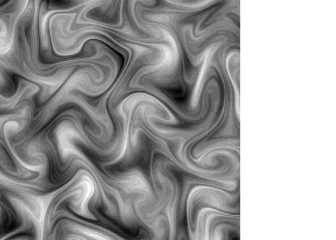
FIG. 4.: Snapshot of the passive scalar field, simultaneous to the vorticity field shown in Fig. 1

To directly check whether small-scale vorticity can be considered as passively advected by velocity, we also solved the equation of transport of passive scalar with a finite lifetime [3, 7, 8]

$${\partial\theta\over\partial t}+{\mbox{\boldmath$v$}}\cdot{\mbox{\boldmath$\nabla$}}\theta=\nu\nabla^{2}\theta-\alpha\theta+f_{\theta}\;.$$ (3)

where the velocity field results from the parallel integration of Eq. (1). The parameters appearing in Eqs. (1)  and (3) are the same, yet the forcings $f_{\omega}$ and $f_{\theta}$ are independent processes with the same statistics. According to the picture drawn above, we expect to observe the same small-scale statistics for $\delta_{r}\omega$ and $\delta_{r}\theta=\theta({\mbox{\boldmath$x$}}+{\mbox{\boldmath$r$}},t)-\theta({\mbox{\boldmath$x$}},t)$.

FIG. 5.: Power spectra of passive scalar ($\times$) and vorticity ($+$). Here $\alpha=0.15$. In the inset we show the same spectra compensated by $k^{1+\zeta^{\theta}_{2}}$.

In Figure 5 we show the power spectra of vorticity, $Z(k)$, and of passive scalar $E_{\theta}(k)$. The two curves are parallel at large $k$, in agreement with the expectation $\zeta^{\omega}_{2}=\zeta^{\theta}_{2}$. We notice that the two spectra do not collapse exactly onto each other. At large scales we observe a big bump in $Z(k)$ around $k=k_{f}$ which has not any correspondent in $E_{\theta}(k)$. This deviation is due to the presence of an inverse energy flux in the Navier-Stokes equation, a phenomenon that has no equivalent in the passive scalar case. Due to this effect, the scaling quality of $S^{\omega}_{p}(r)$ is poorer than the $S^{\theta}_{p}(r)$ one, and a direct comparison of scaling exponents in physical space is even more difficult.

FIG. 6.: Probability density functions of vorticity differences ($+$) and of passive scalar ones ($\times$), normalized by their respective standard deviation, at different scales $r$ within the scaling range.

However, we observe in Fig. 6 that the probability density functions of vorticity and passive scalar increments, once rescaled by their root-mean-square fluctuation, collapse remarkably well onto each other. That proves, along with the result $\zeta^{\omega}_{2}=\zeta^{\theta}_{2}$ obtained from Fig 5, the equality of scaling exponents of vorticity and passive scalar at any order: $\zeta^{\omega}_{p}=\zeta^{\theta}_{p}$.

The actual values can be directly extracted from the statistics of the passive scalar, which is not spoiled by large-scale objects. In Fig. 7 we plot the first exponents $\zeta^{\theta}_{p}$ as obtained by looking at the local slopes of the structure functions $S_{p}^{\theta}(r)$. The numerical values for $\zeta^{\theta}_{p}$ are validated by the almost perfect agreement with the Lagrangian exit-time statistics.

In conclusion, we have shown that in presence of linear friction the small scale vorticity fluctuations in two dimensional direct cascade are intermittent. Intermittency is a consequence of the the competition between exponential separation of Lagrangian trajectories and exponential decay of fluctuations due to friction. Small-scale vorticity fluctuations behave statistically as a passive scalar, as it has been confirmed by a direct comparison. The smoothness of the velocity field appears to be a crucial ingredient for the equality of active and passive scalar statistics.

FIG. 7.: The scaling exponents of the passive scalar $\zeta^{\theta}_{p}$ ($+$). We also show the exponents obtained from the exit times statistics ($\odot$) according to $\langle\exp[-\alpha pT_{L}(r)]\rangle\sim r^{\zeta_{p}^{\theta}}$ with average over about $2\times 10^{5}$ couple of Lagrangian particles. The errorbars are estimated by the r.m.s. fluctuation of the local slope. In the inset we plot the Cramer function $G(\gamma)$ computed from finite time Lyapunov exponents (symbols) and exit time statistics (line).

This work was supported by EU under the contracts HPRN-CT-2000-00162 and FMRX-CT-98-0175. Numerical simulations have been performed at IDRIS (projects 011226 and 011411) and at CINECA (INFM Parallel Computing Initiative).

REFERENCES

- [1] R. Salmon, Geophysical Fluid Dynamics, Oxford University Press, New York, USA (1998). Other well known examples are the Rayleigh friction in stratified fluids, the Hartmann friction in MHD (J. Sommeria, J. Fluid Mech. 170, 139 (1986)) and the friction induced by surrounding air in soap films (M. Rivera and X.L. Wu, Phys. Rev. Lett. 85, 976 (2000)).
- [2] K. Nam, E. Ott, T.M. Antonsen, P.N. Guzdar, Phys. Rev. Lett. 84, 5134 (2000).
- [3] M. Chertkov, Phys. of Fluids, 10, 3017 (1998).
- [4] D. Bernard, Europhys. Lett. 50, 333 (2000).
- [5] E. Ott, Chaos in Dynamical Systems, Cambridge University Press, Cambridge, UK (1993).
- [6] T. Bohr, M.H. Jensen, G. Paladin and A. Vulpiani, Dynamical Systems Approach to Turbulence, Cambridge University Press, Cambridge, UK (1998).
- [7] K. Nam, T.M. Antonsen, P.N. Guzdar, E. Ott, Phys. Rev. Lett. 83, 3426 (1999).
- [8] Z. Neufeld, C. Lopez, E. Hernandez-Garcia, T. Tel, Phys. Rev. E.,61, 3857 (2000)