Spectral Statistics of Rectangular Billiards with Localized Perturbations

Abstract

The form factor $K(\tau)$ is calculated analytically to the order $\tau^{3}$ as well as numerically for a rectangular billiard perturbed by a $\delta$-like scatterer with an angle independent diffraction constant, $D$. The cases where the scatterer is at the center and at a typical position in the billiard are studied. The analytical calculations are performed in the semiclassical approximation combined with the geometrical theory of diffraction. Non diagonal contributions are crucial and are therefore taken into account. The numerical calculations are performed for a self adjoint extension of a $\delta$ function potential. We calculate the angle dependent diffraction constant for an arbitrary perturbing potential $U({\bf r})$, that is large in a finite but small region (compared to the wavelength of the particles that in turn is small compared to the size of the billiard). The relation to the idealized model of the $\delta$-like scatterer is formulated. The angle dependent diffraction constant is used for the analytic calculation of the form factor to the order $\tau^{2}$. If the scatterer is at a typical position, the form factor is found to reduce (in this order) to the one found for angle independent diffraction. If the scatterer is at the center, the large degeneracy in the lengths of the orbits involved leads to an additional small contribution to the form factor, resulting of the angle dependence of the diffraction constant. The robustness of the results is discussed.

I Introduction

The spectral properties of quantum mechanical systems are closely related to the ones of their classical counterparts [1, 2]. This relation can be made precise and quantitative in the semiclassical limit. In the extreme cases this correspondence is quite well understood, although some important details are subject of research [3, 4, 5, 6]. The spectral statistics exhibit a high degree of universality, although there are exceptional systems that do not exhibit this universal behavior, due to some special properties. When a classical system is chaotic the statistical properties of corresponding quantum spectrum are well described by Random Matrix Theory (RMT) [7] with the symmetry determined by the underlying Hamiltonian. For integrable systems, on the other hand, levels are typically uncorrelated resulting in Poissonian spectral statistics [8]. There are however intermediate situations. One is of mixed systems, where in some parts of phase space the motion is chaotic and in other parts it is regular leading to different statistics [9, 10]. Another type of systems that exhibit intermediate statistics are systems with singularities, that are integrable in absence of these singularities. These are models of physical situations where an integrable system is strongly perturbed in a region much smaller then the wavelength of the quantum particle. Examples of such systems are billiards with flux lines, sharp corners and $\delta$-like interactions [11, 12, 13, 14, 15, 16]. The specific system that will be analyzed in the present work is a billiard with a $\delta$-like potential perturbation.

The interest in billiards of various types is primarily theoretical since it is relatively easy to analyze them analytically and numerically. Billiards were studied also experimentally for electrons [17, 18], microwaves [19, 20, 21] and for laser cooled atoms [22, 23]. We hope that in the future, perturbations of the type discussed in the present work will be also introduced in the experimental realizations of billiards.

Semiclassical methods provide a convenient path to explore how classical dynamical properties affect the quantum spectral statistics. The connection between spectral statistics and classical dynamics is usually made using trace formulas which connect the quantum density of states to a sum over classical periodic orbits. For classically chaotic systems the trace formula was developed by Gutzwiller [24, 25] while for classically integrable systems the trace formula was developed by Berry and Tabor [26]. Such formulas can be used to compute the energy level-level correlation function, $R_{2}(\eta)$, where $\eta$ is the level separation. Its Fourier transform is the spectral form factor $K(\tau)$, where the “time” $\tau$ is conjugate to $\eta$. For systems with strong perturbations on length scales smaller than the wavelength, standard semiclassical theory cannot be used and diffraction effects have to be taken into account. For billiards with localized perturbations this can be done in the framework of the Geometrical Theory of Diffraction (GTD) [27]. In this approximation, scattering from the perturbation can be described by a free propagation to the perturbation multiplied by a diffraction constant, which depends on the incoming and outgoing directions, and then free propagation away from the perturbation.

The spectral statistics of the rectangular billiard with a flux line was recently studied [15, 16]. In this system the flux line affects the amplitudes of the contributions of periodic orbits. When the form factor is computed it is found that at small times $\tau$ it tends to a flux dependent constant (instead of $1$ in absence of the flux). Certain triangular billiards were shown to have similar behavior [16]. The works mentioned above are based only on the contributions from periodic orbits. It is of interest to include the contributions of orbits that are diffracted by the flux line in the spectral form factor. The contribution of diffracting orbits turns out to be rather complicated. The contribution of orbits with one diffraction was computed by Sieber [28], while Bogomolny, Pavloff and Schmit computed the contributions of diffracting orbits with several forward diffractions to the density of states [29]. The effect of diffraction on the spectral statistics in these systems was not determined yet. The difficulty results from the need to know the contributions of orbits which diffract almost in the forward direction and to include all of these in the form factor, and this has not been done so far. Since the diffraction from flux lines and corners is complicated it is of special interest to examine a system in which the diffraction is relatively simple. A class of such systems, that consists of integrable billiards with localized perturbations, is the subject of the present work. For systems of this type only diffraction effects are responsible for deviation of the behavior from the one of integrable systems, therefore these are most appropriate for the exploration of such effects.

The diagonal approximation, where the cross terms between the contributions of classical orbits are ignored because of rapidly varying phases associated with them, is used for a large variety of systems. Berry has shown that using the diagonal approximation leads to agreement with the form factor of random matrices, at small times [30]. Only recently Sieber and Richter [31] were able to go beyond the diagonal approximation and to compute the next power of $\tau$ for chaotic systems with time reversal symmetry. This non diagonal contribution was found to originate from orbits with small angle self intersections and orbits which are close to them in coordinate space, except near the intersection. Such configurations are not possible if there is no time reversal symmetry, thus this is an example where the difference in the spectral statistics is connected to a difference in the dynamical properties of the classical counterpart, and the difference can be obtained directly from a formula involving the classical periodic orbits. For chaotic systems with singular perturbations, where effects of diffraction are important, also the non diagonal contributions to the form factor $K(\tau)$ are important. The final result, however, is that such perturbations do not affect the spectral statistics as is clear from the works of Sieber [32, 33] and of Bogomolny, Leboeuf and Schmit [34].

In contrast to the case of chaotic systems, addition of a localized scatterer, is expected to change qualitatively the spectral properties of integrable systems. Moreover, for such systems the diagonal approximation is not sufficient to obtain any interesting physics and one should go beyond this approximation. Non diagonal contributions can be calculated following a method that was developed by Bogomolny [35]. By this method contributions of some manifolds consisting of orbits that are almost parallel are calculated. If a point interaction, that is a generalization of a $\delta$-function potential, is added to a rectangular billiard, one obtains the so called Šeba billiard [11]. The spectral statistics of this system were computed exactly, subject to the assumption that the underlying integrable system exhibits Poissonian statistics [13] and it was shown not to be those of integrable or chaotic systems. The spectral statistics of the Šeba billiard with periodic boundary conditions were shown by Berkolaiko, Bogomolny and Keating [36] to be identical to those of certain star graphs, where the form factor was calculated by Berkolaiko and Keating [37].

After the work was completed a paper by Bogomolny and Giraud [38], where the expansion of $K(\tau)$, was calculated to all orders in $\tau$ was published on the Web. It is more general than the present paper, but in our paper more of the physical properties are calculated and discussed in detail. The methodology of the derivation is different. A comparison between various results of these two papers is presented in App. E.

Generalized $\delta$-functions were extensively studied in mathematical physics in the framework of the self adjoint extension theory [39, 40, 41, 42, 43, 44, 45, 46, 47, 48, 49]. The calculations in [13, 36] were performed within this framework. In the present work also a potential of finite small extension $a$ is studied, under the assumption that $a$ is much smaller than the wavelength of the quantum particle, that in turn is much smaller than the dimensions of the billiard. The relation of the $\delta$-like scatterers to well defined potentials is discussed in the paper.

The aim of this work is to use periodic and diffracting orbits to compute the form factor of rectangular billiards with localized perturbations. The calculation includes non diagonal contributions and leads to a power expansion of $K(\tau)$ where only the first three powers of $\tau$ are calculated. The structure of this paper is as follows. In Sec. II the form factor is calculated for angle independent diffraction. In Sec. III the model of point $\delta$-like interactions is presented, in order to introduce a simple example of angle independent scattering. For this model the results of Sec. II are compared to numerical results in Sec. IV. The scattering from localized potentials that are physically well defined is studied in Sec. V, where it is shown how to compute the diffraction constant in the limit where the size of the perturbation is smaller than the wavelength. In Sec. VI the form factor for angle dependent scattering, with the diffraction constant that was calculated Sec.  V, is computed. The results are summarized and discussed in Sec. VII.

II The Form Factor of a point-like S wave Scatterer

In this section the form factor will be calculated for a rectangular billiard with a scatterer such that its diffraction constant $D$, is angle independent. The form factor is

$$K(\tau)=\int_{-\infty}^{\infty}d\eta R_{2}(\eta)e^{2\pi i\eta\tau},$$ (1)

where $R_{2}(\eta)$ is the energy levels correlation function:

$$R_{2}(\eta)=\left\langle d_{osc}\left(E-\frac{\eta\Delta}{2}\right)d_{osc}\left(E+\frac{\eta\Delta}{2}\right)\right\rangle\Delta^{2}$$ (2)

and $\Delta$ denotes the mean level spacing of the system. The brackets denote averaging over an energy window which is large compared to the mean level spacing $\Delta$ but small when compared to the semiclassical energy $E$. In the semiclassical limit, the oscillatory part of the density of states, $d_{osc}(E)\equiv d(E)-\langle d(E)\rangle$, is of the form

$$d_{osc}(E)\simeq\sum_{p}A_{p}e^{i\frac{S_{P}}{\hbar}}+c.c.,$$ (3)

where $c.c.$ denotes the complex conjugate and the sum is over periodic orbits. Using this density of states, the form factor is given by:

$$K(\tau)=2\pi\hbar\Delta\left\langle\sum_{pp^{\prime}}A_{p}A_{p^{\prime}}^{*}e^{\frac{i}{\hbar}(S_{p}-S_{p^{\prime}})}\delta\left(\frac{2\pi\hbar}{\Delta}\tau-\frac{t_{p}+t_{p^{\prime}}}{2}\right)\right\rangle$$ (4)

where $S_{p}$ is the action of the orbit, $t_{p}$ is its period, and $\tau>0$ is assumed. The sum is over the leading semiclassical contributions to the density of states. For smooth potentials $d_{osc}$ is given by the Berry-Tabor formula for integrable systems [26] and by the Gutzwiller trace formula for chaotic systems [24, 25]. In these formulas the sum is over the periodic orbits of the system. In the present work, periodic orbits and diffracting orbits will be included in the sum.

Due to the averaging only action differences that are of the order of $\hbar$ or less can contribute to the form factor. As a result, the diagonal approximation can be used, where only pairs of orbits with the same action contribute. This approximation is valid for integrable systems [30] and thus also valid when there are only once diffracting orbits (since their density is proportional to that of periodic orbits as will be explained in the following). When orbits with more than one diffraction are included this approximation is no longer valid and non diagonal terms should be included as is done in what follows. Since the motion in the billiard is free, the periods of the orbits are related to the lengths by $t_{p}=\frac{l_{p}}{2k}$ where $k=\sqrt{E}$ is the wavenumber (the units $\hbar=1$, $2m=1$ are used from now). The mean level spacing , in the semiclassical limit, is given by $\Delta=\frac{4\pi}{\cal A}$. In the diagonal approximation the form factor is expressed as a sum over orbits of identical lengths

$$K(\tau)=\sum_{p}\frac{16\pi^{2}k}{\cal A}\left\langle|A_{p}|^{2}\delta(\l_{p}-{\cal A}k\tau)\right\rangle.$$ (5)

The averaging widens the delta function and enables to replace the sum over orbits by an integral using the density of orbits. Every factor of length, $l_{p}$, is replaced by a factor of ${\cal A}k\tau$, and as will be seen, every diffraction order eventually contributes a power of $\tau$ to the from factor. The form factor $K(\tau)$ will be calculated to the third order in $\tau$.

The spectral statistics are very sensitive to the location of the scatterer, since they are influenced by degeneracies in the lengths of the diffracting orbits. Therefore we choose to treat first the simplest case when the scatterer is in the center of the rectangle. Then length degeneracies are maximal. Later we treat the case in which the scatterer is at a typical location, such that its coordinates (relative to the rectangle sides) are typical irrational numbers.

A Scatterer at the center

The periodic and diffracting orbits are classified by the number of bounces from the boundaries. We will denote by ${\bf N}_{p}=(N_{p},M_{p})$ a periodic orbit with $2N_{p}$ and $2M_{p}$ bounces from the boundaries and by ${\bf N}_{j}=(N_{j},M_{j})$ a diffracting orbit with $N_{j}$ and $M_{j}$ bounces from the boundary. When the scatterer is at the center of the rectangle the length of the diffracting segments is given by

$$l_{j}=\sqrt{a_{x}^{2}N_{j}^{2}+a_{y}^{2}M_{j}^{2}}$$ (6)

while the length of the periodic orbits is

$$l_{p}=2\sqrt{a_{x}^{2}N_{p}^{2}+a_{y}^{2}M_{p}^{2}}$$ (7)

where $a_{x}$ and $a_{y}$ are the lengths of the sides of the rectangle.

The contributions to the oscillatory part of the density of states were calculated in the framework of geometrical theory of diffraction in App. A. For an angle independent scatterer the contributions (A30) to $d_{osc}$ can be simplified since $D(\theta,\theta^{\prime})$ reduces to a constant $D$ and if the scatterer is at the center the terms do not depend on $\mu$ and $\nu$. The contribution of them with no more than three diffractions is

$$d_{osc}(E)=\sum_{p}A_{p}^{(0)}e^{ikl_{p}}+\sum_{j}A_{j}^{(1)}e^{ikl_{j}}+\sum_{j_{1},j_{2}}A_{j_{1},j_{2}}^{(2)}e^{ik(l_{j_{1}}+l_{j_{2}})}+\sum_{j_{1},j_{2},j_{3}}A_{j_{1},j_{2},j_{3}}^{(3)}e^{ik(l_{j_{1}}+l_{j_{2}}+l_{j_{3}})}+c.c.+\cdots$$ (8)

where

$$A_{p}^{(0)}=\frac{2{\cal A}}{\pi\sqrt{8\pi kl_{p}}}e^{-i\frac{\pi}{4}},$$ (9)

$$A_{j}^{(1)}=\frac{(-1)^{N_{j}+M_{j}}\sqrt{l_{j}}}{\pi k\sqrt{8\pi k}}De^{-i\frac{3}{4}\pi},$$ (10)

$$A_{j_{1},j_{2}}^{(2)}=(-1)^{N_{j_{1}}+M_{j_{1}}+N_{j_{2}}+M_{j_{2}}}\frac{l_{j_{1}}+l_{j_{2}}}{4\pi^{2}k^{2}\sqrt{l_{j_{1}}l_{j_{2}}}}D^{2}e^{-i\frac{3}{2}\pi}$$ (11)

and

$$A_{j_{1},j_{2},j_{3}}^{(3)}=(-1)^{N_{j_{1}}+M_{j_{1}}+N_{j_{2}}+M_{j_{2}}+N_{j_{3}}+M_{j_{3}}}\frac{16D^{3}}{3\pi k(8\pi k)^{\frac{3}{2}}}\frac{l_{j_{1}}+l_{j_{2}}+l_{j_{3}}}{\sqrt{l_{j_{1}}l_{j_{2}}l_{j_{3}}}}e^{-i\frac{\pi}{4}}.$$ (12)

We omitted the factors $\beta_{j}$ defined in (A15) since the fraction of orbits where these differ from unity is negligible in the calculations of the present section. Examples of the various orbits contributing to (8-11) are presented in Fig. 1.

FIG. 1.: Several orbits contributing to the density of states: a) a periodic orbit (the ($1,1$) orbit), b) a forward once diffracting orbit ($2,2$), c) a once diffracting orbit ($2,1$), and d) a twice diffracting orbit.

First the contribution of terms that involve no more than one diffraction, resulting from the first two terms in the expansion (8) of $d_{osc}$, will be calculated. Following (A18) the contributions of the diffracting terms can be classified according the parity of $N_{j}$ and $M_{j}$. If both $N_{j}$ and $M_{j}$ are even (even-even orbits) the orbit $j$ coincides with a periodic orbit, since in the notation of (A18), at the scatterer $\theta_{in}=\theta_{out}$ (compare Fig. 1 a) and b)) and the contribution of these orbits will be calculated first. There is no such relation for the other parities, (even-odd, odd-even, odd-odd, referring to the parities of $N_{j}$ and $M_{j}$) and actually for such parities the diffracting orbits are halves of periodic orbits (this is only true if the scatterer is at the center, therefore for example the orbit in Fig. 1 c) is not a half of a ($2,1$) periodic orbit). For even-even diffracting orbits the first two sums in the expression (8) can be grouped as

$$d_{osc}^{(1)}(E)=\sum_{p}\tilde{A}_{P}e^{ikl_{p}}+\sum_{j}A_{j}^{(1)}e^{ikl_{j}}+c.c.$$ (13)

where the first sum runs over periodic orbits while the second sum runs over diffracting orbits, omitting orbits where both $N_{j}$ and $M_{j}$ are even and

$$\tilde{A}_{p}=\left(\frac{2{\cal A}}{\pi\sqrt{8\pi kl_{p}}}+\frac{\sqrt{l_{p}}}{\pi k\sqrt{8\pi k}}De^{-i\frac{\pi}{2}}\right)e^{-i\frac{\pi}{4}}.$$ (14)

The diagonal approximation is now applied to various terms in (13) and the sum in (5) is replaced by an integral with the density

$$\rho(l)=\frac{\pi l}{8{\cal A}}$$ (15)

of orbits of length $l$. This is the density of periodic orbits as well as the density of diffracting orbits with a given parity of $N_{j}$ and $M_{j}$ as can be easily seen from (6) and (7). The resulting contribution of the periodic and even-even diffracting orbits to the form factor is

$$K^{(1,e)}(\tau) =\frac{16\pi^{2}k}{{\cal A}}\int_{0}^{\infty}dl\frac{\pi l}{8{\cal A}}\left(\frac{{\cal A}^{2}}{2\pi^{3}kl}+\frac{{\cal A}}{2\pi^{3}k^{2}}\Im D+\frac{l}{8\pi^{3}k^{3}}|D|^{2}\right)\delta(l-{\cal A}k\tau)$$ (16)

$$=1+\Im D\tau+\frac{|D|^{2}}{4}\tau^{2}.$$ (17)

The contribution of the other diffracting orbits (odd-odd, odd-even, even-odd) with the amplitudes $A_{j}^{(1)}$ of (10) are

$$K^{(1,o-o)}(\tau)=K^{(1,o-e)}(\tau)=K^{(1,e-o)}(\tau)=\frac{|D|^{2}\tau^{2}}{4}$$ (18)

and their combined contribution is

$$K^{(1,o)}(\tau)=\frac{3|D|^{2}\tau^{2}}{4}.$$ (19)

Thus, the contribution of the once-diffracting orbits and the periodic orbits to the form factor is

$$K^{(1)}(\tau)=K^{(1,e)}(\tau)+K^{(1,o)}(\tau)=1+\Im D\tau+|D|^{2}\tau^{2}.$$ (20)

From (9-11) we note that the powers of $\frac{1}{\sqrt{k}}$ and $\sqrt{l_{j}}$ (the powers in (9-11) combined with the increasing density of multiple diffracting orbits resulting from powers of (15)) increase with the powers of $D$ and by (4) and (5) these lead to increasing orders of $\tau$. We are interested first in all contributions to the order $\tau^{2}$. The additional terms that may contribute to this order result from non diagonal terms in (4) where $p$ is a periodic orbit and $j^{\prime}$ is an orbit with two diffractions, namely terms of the form

$$A_{p}A_{j^{\prime}}^{*}e^{\frac{i}{\hbar}(S_{p}-S_{j^{\prime}})}=A_{p}A_{j_{1},j_{2}}^{(2)*}e^{ik(l_{p}-l_{j_{1}}-l_{j_{2}})}.$$ (21)

The contribution of such terms will be analyzed in the following. All other contributions are of higher order in $\tau$.

We turn to analyze the contribution of non diagonal terms involving periodic and twice diffracting orbits. These oscillate as $e^{ik(l_{p}-l_{j_{1}}-l_{j_{2}})}$ that may be potentially fast. Naively, one can guess that after smoothing, the contributions relevant to the form factor are those for which $l_{p}=l_{j_{1}}+l_{j_{2}}$. However, it turns out that there are not enough orbits that satisfy this equality in order to compensate for the extra factor of $1/k$ due to the additional diffraction. The contribution comes from combinations of orbits for which the lengths are almost equal. Such combinations survive since there are enough orbits for which the phase of the exponent is of the order of unity in the semiclassical limit. This is caused by the fact that these orbits have hidden saddle manifolds on which their action differences are slowly varying. These manifolds were identified by Bogomolny [35], and were used to compute the density-density correlation function and mean values of powers of Green’s functions for integrable systems. The diffraction problem discussed here has lengths (or actions) that are related to the length of the periodic orbits so that saddle manifolds exist. We use Bogomolny’s method to compute this contribution. It will be convenient to expand the length of the diffracting orbits around the length of orbits that satisfy $l_{p}=l_{j_{1}}+l_{j_{2}}$. This expansion is given by

$$l_{j} = \sqrt{a_{x}^{2}(N_{j}+\delta N_{j})^{2}+a_{y}^{2}(M_{j}+\delta M_{j})^{2}}\simeq\sqrt{a_{x}^{2}N_{j}^{2}+a_{y}^{2}M_{j}^{2}}$$ (23)

$$+\frac{1}{\sqrt{a_{x}^{2}N_{j}^{2}+a_{y}^{2}M_{j}^{2}}}(a_{x}^{2}N_{j}\delta N_{j}+a_{y}^{2}M_{j}\delta M_{j})+\frac{a_{x}^{2}a_{y}^{2}}{2(a_{x}^{2}N_{j}^{2}+a_{y}^{2}M_{j}^{2})^{\frac{3}{2}}}(M_{j}\delta N_{j}-N_{j}\delta M_{j})^{2}.$$

The length difference in the exponent is

$$\delta l_{p}=l_{j_{1}}+l_{j_{2}}-l_{p}$$ (24)

The periodic orbit is not expanded because for each periodic orbit there will be a saddle manifold composed of different twice-diffracting orbits. The summation over the orbits in the manifold will be also combined with summation over all of the periodic orbits. Equivalently, it is possible to fix any of the lengths, expand the other lengths, and to reach the same contribution to the form factor.

The condition that the orbits are on the saddle manifold is that the length difference, $\delta l_{p}$, is stationary leading to:

$$\frac{1}{\sqrt{a_{x}^{2}N_{j_{1}}^{2}+a_{y}^{2}M_{j_{1}}^{2}}}(a_{x}^{2}N_{j_{1}}\delta N_{j_{1}}+a_{y}^{2}M_{j_{1}}\delta M_{j_{1}})+\frac{1}{\sqrt{a_{x}^{2}N_{j_{2}}^{2}+a_{y}^{2}M_{j_{2}}^{2}}}(a_{x}^{2}N_{j_{2}}\delta N_{j_{2}}+a_{y}^{2}M_{j_{2}}\delta M_{j_{2}})=0.$$ (25)

The orbits on the manifold are the integer solutions of this equation. Since the aspect ratio of the rectangle is assumed to be a typical irrational number, such solutions can be found only if the orbits are related by

$$\frac{\sqrt{a_{x}^{2}N_{j_{1}}^{2}+a_{y}^{2}M_{j_{1}}^{2}}}{\sqrt{a_{x}^{2}N_{j_{2}}^{2}+a_{y}^{2}M_{j_{2}}^{2}}}=\frac{r_{j_{1}}}{r_{j_{2}}}.$$ (26)

This means that the orbits are repetitions of some simpler orbit, for example

$$\sqrt{a_{x}^{2}N_{j_{1}}^{2}+a_{y}^{2}M_{j_{1}}^{2}}=r_{j_{1}}\sqrt{a_{x}^{2}n^{2}+a_{y}^{2}m^{2}}=r_{j_{1}}l_{0}.$$ (27)

Substituting this condition in (25) leads to

$$a_{x}^{2}n\delta N_{j_{1}}+a_{x}^{2}n\delta N_{j_{2}}+a_{y}^{2}m\delta M_{j_{1}}+a_{y}^{2}m\delta M_{j_{2}}=0.$$ (28)

Since the aspect ratio is a typical irrational number an integer solution can be found only if

$$\delta M_{j_{1}} = -\delta M_{j_{2}}$$ (29)

$$\delta N_{j_{1}} = -\delta N_{j_{2}}.$$ (30)

We are interested in the contribution that survives the energy averaging, required for contributions to the form factor. Therefore we will consider the saddle manifold for which

$$l_{p}=2\sqrt{a_{x}^{2}N_{p}^{2}+a_{y}^{2}M_{p}^{2}}=(r_{j_{1}}+r_{j_{2}})l_{0}.$$ (31)

This condition states that the periodic orbit (which will contribute) is also proportional to $(n,m)$ and $l_{p}=2r_{p}l_{0}$ with

$$2r_{p}=r_{j_{1}}+r_{j_{2}}$$ (32)

is satisfied.

The contribution of the terms of this saddle manifold to the level-level correlation function $R_{2}(\eta)$ is:

$${R^{\prime}}_{2}^{(2)}(\eta)=\left\langle\sum_{p,j_{1},j_{2}}\frac{2{\cal A}}{\pi\sqrt{8\pi l_{p}k}}e^{-i\frac{\pi}{4}}\frac{l_{j_{1}}+l_{j_{2}}}{4\pi^{2}k^{2}\sqrt{l_{j_{1}}l_{j_{2}}}}e^{i\frac{3\pi}{2}}e^{ik(l_{p}-l_{j_{1}}-l_{j_{2}})}D^{2}e^{i\frac{\eta\Delta}{4k}(l_{j_{1}}+l_{j_{2}}+l_{p})}\right\rangle\Delta^{2}$$ (33)

$$+c.c.+\left(\eta\rightarrow-\eta\right).$$ (34)

The symbol $\left(\eta\rightarrow-\eta\right)$ denotes two terms similar to the first ones but with the opposite sign of $\eta$. This is actually a sum over $(N_{p},M_{p})$, $(N_{j_{1}},M_{j_{1}})$ and $(N_{j_{2}},M_{j_{2}})$ that define the orbits $p$, $j_{1}$ and $j_{2}$ respectively. The contributions with similar phases, that do not cancel each other, and therefore survive the averaging over energy involved in the calculation of the form factor are those that satisfy (29) and (32). The sum will be calculated and then Fourier transformed in order to obtain the corresponding contribution to the form factor. The dominant contributions are these in which the length difference $\delta l_{p}$ is much smaller than unity. The configuration of these contribution is shown in Fig. 2.

FIG. 2.: The configuration of lengths on the saddle manifold

The two diffracting segments are almost parallel to the periodic orbit. Such a configuration is allowed since the difference between any lattice points is also a lattice point, moreover, the conditions (29), (32) force the orbit to have this configuration. Note that $l_{1},l_{2}$ are the projections of the lengths of the diffracting segments on the direction of the periodic orbit (to the leading order in $\delta\phi_{j}$). Since they are almost parallel they are a good approximation to the lengths of the diffracting segments.

Since the contributing orbits have the configuration of Fig. 2, the variables $l_{1}$ and $t$ are convenient coordinates. This choice also takes into account the conditions (29) and (32). The length difference is given by

$$\delta l_{p}=l_{j_{1}}+l_{j_{2}}-l_{p}\simeq\frac{1}{2}t^{2}\left(\frac{1}{l_{1}}+\frac{1}{l_{2}}\right)-\frac{1}{8}t^{4}\left(\frac{1}{l_{1}^{3}}+\frac{1}{l_{2}^{3}}\right)$$ (35)

where $l_{2}=l_{p}-l_{1}$. The length difference $\delta l_{p}$ appears as a phase in an exponent multiplied by $k$. Thus only length differences which scale as $\frac{1}{k}$ can contribute to the correlation function. The lengths of orbits that will contribute to the form factor scale as $k$ and thus the corresponding values of $t$ are of the order of unity or less. Since the sum is dominated by terms in which $t\sim 1$ or less, the expansion (35) is justified. This expansion may break down when either $l_{1}\rightarrow 0$ or $l_{2}\rightarrow 0$. However, there is a minimal length for the diffracting orbits and such lengths do not occur in the sum.

The correlation function is computed by replacing the sum over orbits by an integral over $l_{1}$ and $t$. The slowly varying terms are replaced by their values on the saddle (when $t=0$) and the phase is replaced by the leading term of (35). To transform the sum into an integral the density of contributions is needed. The configuration in Fig. 2 is obtained when the plane is tiled with rectangles using reflections with respect to the hard walls. The scatterer is also reflected and its images form a lattice (since there is a scatterer in the center of each rectangle). An example for this unfolding is presented in Fig. 3 (for a scatterer which is not at the center).

FIG. 3.: Unfolding of orbits using reflections around the rectangle boundaries.

The ($1,2$) orbit in the original rectangle (solid line) is equivalent to the one connecting the scatterer with its image (dashed line). The density of points in this lattice is $\frac{1}{\cal A}$. After these manipulations the correlation function is given by

$$R^{{}^{\prime}(2)}_{2}(\eta)= \left\langle\sum_{p}\int_{0}^{l_{p}}dl_{1}\int dt\;\frac{2}{\pi\sqrt{8\pi l_{p}k}}e^{-i\frac{\pi}{4}}\frac{l_{1}+l_{2}}{4\pi^{2}k^{2}\sqrt{l_{1}l_{2}}}e^{i\frac{3\pi}{2}}e^{i\frac{\eta\Delta}{4k}(l_{1}+l_{2}+l_{p})}D^{2}e^{-i\frac{kt^{2}}{2}\left(\frac{1}{l_{1}}+\frac{1}{l_{2}}\right)}\right\rangle\Delta^{2}$$ (36)

$$+c.c+(\eta\rightarrow-\eta).$$ (37)

Calculation of the Gaussian integral leads to

$$R^{{}^{\prime}(2)}_{2}(\eta)=\left\langle\sum_{p}\frac{l_{p}}{2\pi^{3}k^{3}}(-\Re D^{2})e^{i\frac{\eta\Delta}{2k}l_{p}}\right\rangle\Delta^{2}+(\eta\rightarrow-\eta).$$ (38)

The Fourier transform leads to the form factor

$$K^{{}^{\prime}(2)}(\tau)=\left\langle\sum_{p}\frac{2\Delta l_{p}}{\pi^{2}k^{2}}\delta\left(l_{p}-\frac{4\pi k\tau}{\Delta}\right)(-\Re D^{2})\right\rangle$$ (39)

where only positive times were taken into account. The sum over periodic orbits is replaced by an integral using the density (15) leading to

$${K^{\prime}}^{(2)}(\tau)=\tau^{2}\Re(-D^{2}),$$ (40)

which is the non diagonal contribution to the form factor. This contribution is indeed of order $\tau^{2}$ as was expected.

After computing all of the contributions of order $\tau^{2}$ we turn to compute the contributions to the form factor which are of order $\tau^{3}$. There are three possible contributions of this order: diagonal contributions from twice diffracting orbits that will be denoted by $K^{(3)}(\tau)$, non diagonal contributions resulting from combinations of once and twice diffracting orbits, denoted by $K^{{}^{\prime}(3a)}(\tau)$, and from combinations of periodic orbits and orbits with three diffractions, denoted by $K^{{}^{\prime}(3b)}(\tau)$. These contributions are computed in the following.

To obtain the diagonal contribution of twice diffracting orbits (8) is substituted in (2), and only the terms with two diffractions are kept. A Fourier transform leads to

$$K^{(3)}(\tau)=\left\langle\sum_{j_{1}j_{2}j_{3}j_{4}}{A^{(2)}_{j_{1}j_{2}}}^{*}A_{j_{3}j_{4}}^{(2)}e^{-ik(l_{j_{1}}+l_{j_{2}}-l_{j_{3}}-l_{j_{4}})}\delta\left(\frac{l_{j_{1}}+l_{j_{2}}+l_{j_{3}}+l_{j_{4}}}{2}-\frac{4\pi k\tau}{\Delta}\right)\right\rangle 4\pi k\Delta$$ (41)

where contributions from negative times were omitted. The diagonal approximation requires that $l_{j_{1}}+l_{j_{2}}=l_{j_{3}}+l_{j_{4}}$, this means that $l_{j_{1}}=l_{j_{3}}$ and $l_{j_{2}}=l_{j_{4}}$ or that $l_{j_{1}}=l_{j_{4}}$ and $l_{j_{2}}=l_{j_{3}}$. Both cases result in identical contributions (the fraction of orbits where $l_{j_{1}}=l_{j_{2}}$ is negligible). Using (11) and replacing the sums by integrals with the density of diffracting segments $\frac{\pi l}{2{\cal A}}$ resulting of multiplication of (15) by $4$, to take account of the various possible parities, leads to

$$K^{(3)}(\tau)=\int_{0}^{\infty}dl_{1}dl_{2}\;\frac{\pi^{2}l_{1}l_{2}}{4{\cal A}^{2}}\frac{(l_{1}+l_{2})^{2}\Delta}{2\pi^{3}k^{3}l_{1}l_{2}}|D|^{4}\delta\left(l_{1}+l_{2}-\frac{4\pi k\tau}{\Delta}\right)=\frac{1}{2}|D|^{4}\tau^{3}.$$ (42)

One should note that there is a non diagonal contribution from combinations of two twice diffracting orbits but this contribution is of higher order in $\tau$.

The contribution which results from combinations of once and twice diffracting orbits is computed along the same lines as that from the combinations from twice diffracting and periodic orbits which was computed earlier. Using (10) and (11), the relevant contribution to the correlation function is found to be given by

$$R_{2}^{{}^{\prime}(3a)}(\eta) = \left\langle\sum_{j_{1}j_{2}j_{3}}(-1)^{N_{j_{1}}+M_{j_{1}}+N_{j_{2}}+M_{j_{2}}+N_{j_{3}}+M_{j_{3}}}\frac{\sqrt{l_{j_{1}}}(l_{j_{2}}+l_{j_{3}})}{4\pi^{3}k^{3}\sqrt{8\pi kl_{j_{2}}l_{j_{3}}}}\left[|D|^{2}D^{*}e^{ik(l_{j_{1}}-l_{j_{2}}-l_{j_{3}})}\right.\right.$$ (43)

$$\times \left.\left.e^{-i\frac{\eta\Delta}{4k}(l_{j_{1}}+l_{j_{2}}+l_{j_{3}})}e^{i\frac{3\pi}{4}}+c.c.+\left(\eta\rightarrow-\eta\right)\right]\rule{0.0pt}{17.07164pt}\right\rangle\Delta^{2}$$ (44)

where $j_{1}$ denotes the once diffracting orbit with length $l_{j_{1}}$ and $j_{2},j_{3}$ denotes the twice diffracting orbit with length $l_{j_{2}}+l_{j_{3}}$. Only combinations of orbits for which $l_{j_{1}}\simeq l_{j_{2}}+l_{j_{3}}$ survive the smoothing. This leads to a saddle manifold of orbits that satisfy $N_{j_{1}}=N_{j_{2}}+N_{j_{3}}$ and $M_{j_{1}}=M_{j_{2}}+M_{j_{3}}$ (note that on this saddle manifold $N_{j_{1}}+N_{j_{2}}+N_{j_{3}}+M_{j_{1}}+M_{j_{2}}+M_{j_{3}}$ is even). To compute this contribution the sum over $j_{2},j_{3}$ is restricted to the saddle manifold, on which the length difference is

$$l_{j_{1}}-l_{j_{2}}-l_{j_{3}}\simeq-\frac{t^{2}}{2l_{2}}-\frac{t^{2}}{2l_{3}}$$ (45)

where $l_{2}+l_{3}=l_{j_{1}}$, in analogy with (35). The summation on the saddle manifold is then replaced by integration over $t,l_{2}$ with density $\frac{1}{{\cal A}}$

$$R_{2}^{{}^{\prime}(3a)}(\tau) = \left\langle\sum_{j_{1}}\int_{0}^{l_{j_{1}}}\!dl_{2}\!\int\!dt\frac{l_{j_{1}}^{\frac{3}{2}}}{4\pi^{3}k^{3}{\cal A}\sqrt{8\pi kl_{2}l_{3}}}\left[|D|^{2}D^{*}e^{-ik\left(\frac{t^{2}}{2l_{2}}+\frac{t^{2}}{2l_{3}}\right)}e^{-i\frac{\eta\Delta}{2k}l_{j_{1}}+i\frac{3\pi}{4}}+\!c.c.\!+\left(\eta\!\rightarrow\!-\eta\right)\right]\right\rangle\Delta^{2}$$ (46)

$$= \left\langle\sum_{j_{1}}\frac{l_{j_{1}}^{2}}{4\pi^{3}k^{4}{\cal A}}|D|^{2}(\Im D)e^{-i\frac{\eta\Delta}{2k}}+\left(\eta\rightarrow-\eta\right)\right\rangle\Delta^{2}.$$ (47)

The contribution to the form factor is obtained by Fourier transforming (46) and replacing the sum over $j_{1}$ by an integral with the density $\frac{\pi l_{1}}{2{\cal A}}$, resulting in

$$K^{{}^{\prime}(3a)}(\tau)=\int_{0}^{\infty}dl_{1}\;\frac{l_{1}^{3}\Delta}{2\pi k^{3}{\cal A}^{2}}|D|^{2}\Im D\delta\left(l_{1}-\frac{4\pi k\tau}{\Delta}\right)=2|D|^{2}\Im D\tau^{3}.$$ (48)

The last contribution to be computed is from combinations of periodic orbits and orbits with three diffractions. The calculation is very similar to the one just performed. Using (9) and (12) the contribution to the correlation function from combinations of periodic orbits and orbits with three diffractions is found to be

$$R_{2}^{{}^{\prime}(3b)}(\eta)=\left\langle\sum_{pj_{1}j_{2}j_{3}}\frac{{\cal A}(l_{j_{1}}+l_{j_{2}}+l_{j_{3}})}{6\pi^{4}k^{3}\sqrt{l_{p}l_{j_{1}}l_{j_{2}}l_{j_{3}}}}\left[(D^{3})^{*}e^{ik(l_{p}-l_{j_{1}}-l_{j_{2}}-l_{j_{3}})}e^{-i\frac{\eta\Delta}{4k}(l_{p}+l_{j_{1}}+l_{j_{2}}+l_{j_{3}})}+c.c.+\left(\eta\rightarrow-\eta\right)\right]\right\rangle\Delta^{2}$$ (49)

where the factor $(-1)^{N_{j_{1}}+N_{j_{2}}+N_{j_{3}}+M_{j_{1}}+M_{j_{2}}+M_{j_{3}}}$ was omitted since on the saddle manifold it reduces to unity. The saddle manifold is composed of orbits which satisfy

$$N_{j_{1}}+N_{j_{2}}+N_{j_{3}} = N_{p}$$ (50)

$$M_{j_{1}}+M_{j_{2}}+M_{j_{3}} = M_{p}.$$ (51)

The dominant contributions to the correlation function are from diffracting segments which are almost parallel to the periodic orbit as is shown in Fig. 4.

FIG. 4.: The configuration of lengths on the saddle manifold composed of periodic orbits and orbits with three diffractions

.

The length difference is given by

$$l_{p}-l_{j_{1}}-l_{j_{2}}-l_{j_{3}}\simeq-\frac{1}{2}\frac{t_{1}^{2}}{l_{1}}-\frac{1}{2}\frac{t_{2}^{2}}{l_{3}}-\frac{1}{2}\frac{(t_{1}-t_{2})^{2}}{l_{2}}.$$ (52)

The summation over $j_{1},j_{2},j_{3}$ in (49) is restricted to the saddle manifold and then replaced by integration over $l_{1},t_{1},l_{2},t_{2}$ where $l_{1}$ varies between $0$ and $l_{p}$ and $l_{2}$ between $0$ and $l_{p}-l_{1}$. When the sums over $j_{1},j_{2}$ are replaced by integrals a factor of $\frac{1}{{\cal A}^{2}}$, resulting from the density of contributions is introduced. The integral over $t_{1},t_{2}$ is Gaussian and can be evaluated

$$\int dt_{1}dt_{2}\;e^{-i\frac{k}{2}\left[\frac{t_{1}^{2}}{l_{1}}+\frac{t_{2}^{2}}{l_{3}}+\frac{(t_{1}-t_{2})^{2}}{l_{2}}\right]}=\frac{2\pi}{ik}\sqrt{\frac{l_{1}l_{2}l_{3}}{l_{p}}}.$$ (53)

The resulting contribution to the correlation function is given by

$$R_{2}^{{}^{\prime}(3b)}(\tau)=\left\langle\sum_{p}\int_{0}^{l_{p}}dl_{1}\int_{0}^{l_{p}-l_{1}}dl_{2}\;\frac{1}{3\pi^{3}k^{4}{\cal A}}\left[-i(D^{3})^{*}e^{-i\frac{\eta\Delta}{2k}l_{p}}+c.c+\left(\eta\rightarrow-\eta\right)\right]\right\rangle\Delta^{2}.$$ (54)

The integrals can be computed and then (54) is Fourier transformed leading to the following contribution to the form factor

$$K^{{}^{\prime}(3b)}(\tau)=-\left\langle\sum_{p}\frac{4\Delta l_{p}^{2}}{3\pi^{2}k^{3}{\cal A}}\Im(D^{3})\delta\left(l_{p}-\frac{4\pi k\tau}{\Delta}\right)\right\rangle.$$ (55)

The sum over periodic orbits can be replaced by an integral using the density (15), leading to

$$K^{{}^{\prime}(3b)}(\tau)=-\frac{2}{3}\Im(D^{3})\tau^{3}.$$ (56)

Combining all the different contributions, that are given by (20), (40), (42), (48) and (56), the form factor is

$$K(\tau)=1+\Im D\tau+\left(|D|^{2}-\Re D^{2}\right)\tau^{2}+\frac{|D|^{4}\tau^{3}}{2}+2|D|^{2}\Im D\tau^{3}-\frac{2}{3}\Im D^{3}\tau^{3}+O(\tau^{4}).$$ (57)

The diffraction is assumed to conserve probability and therefore the diffraction constant has to satisfy the optical theorem. For an angle independent scatterer in two dimensions it takes the form:

$$\Im D=-\frac{|D|^{2}}{4},$$ (58)

leading to

$$|D|^{4}=8(|D|^{2}-\Re D^{2}).$$ (59)

With the help of the last equations (57) can be simplified to

$$K(\tau)=1-\frac{|D|^{2}}{4}\tau+\frac{1}{8}|D|^{4}\tau^{2}+\left(\frac{1}{2}|D|^{4}-\frac{1}{24}|D|^{6}\right)\tau^{3}+O(\tau^{4}).$$ (60)

The term linear in time results from the combination of (forward) diffracting orbits and periodic orbits and is related, by the optical theorem, to the total cross section of the scatterer and thus its sign is always negative. The resulting form factor is $1$ at $\tau=0$ and decreases with $\tau$ due to the scatterer. At larger $\tau$ the form factor starts to rise, and will get back to $1$ for large $\tau$ since the spectrum is discrete [30]. Qualitatively, this type of behavior should be observed for integrable systems with point perturbations, since the forward diffracting orbits are always on a family of periodic orbits. From the terms to order $\tau^{2}$ one may get the wrong impression that the form factor depends on $D$ and $\tau$ only via the combination $|D|^{2}\tau$ and in particular its value at the minimum is independent of $|D|$. This is not correct as one finds from the term of order $\tau^{3}$. In particular the expansion exhibits dependence on $|D|^{2}$ of the minimum that is found reasonable compared to the numerical calculations presented in Sec. IV. For this reason the calculation was terminated at the order $\tau^{3}$. We now turn to the case where the scatterer is located at some typical (irrational) position. Only slight modifications of the calculation are needed, and these are related to the lifting of length degeneracies.

B Scatterer at a typical position

When the scatterer is in the center of the rectangle the lengths of all the diffracting orbits with the same indices ${\bf N}_{1}$ were the same. If the scatterer is not in the center this is no longer true. An example is given in Fig. 5.

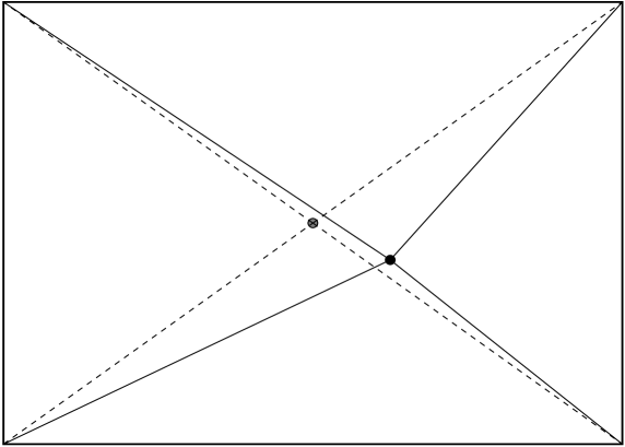
FIG. 5.: All $(1,1)$ diffracting orbits for various scatterer positions

The four dashed lines in Fig. 5 represent the four $(1,1)$ once diffracting orbits which go from the scatterer to a corner and then back, they all have equal lengths. When the scatterer is not in the center the orbits with the same index $(N_{j},M_{j})$ (solid lines) have different lengths. This situation is typical for odd-odd orbits (orbits where both $N_{j}$ and $M_{j}$ are odd). If the scatterer is shifted by $(a_{x}\delta_{x},a_{y}\delta_{y})$ from the center the lengths of the odd-odd $(N_{j},M_{j})$ orbits take all four values $l_{j}^{(o,o)}=\sqrt{a_{x}^{2}(N_{j}\pm 2\delta_{x})^{2}+a_{y}^{2}(M_{j}\pm 2\delta_{y})^{2}}$. It will be assumed in what follows that $\delta_{x}$ and $\delta_{y}$ are typical irrational numbers, therefore the various lengths are not related in any simple way. For even-odd orbits the lengths take the two values $l_{j}^{(e,o)}=\sqrt{a_{x}^{2}N_{j}^{2}+a_{y}^{2}(M_{j}\pm 2\delta_{y})^{2}}$ while for odd-even orbits the lengths take the two values $l_{j}^{(o,e)}=\sqrt{a_{x}^{2}(N_{j}\pm 2\delta_{x})^{2}+a_{y}^{2}M_{j}^{2}}$. From (A18) one sees that these are related by time reversal symmetry. For even-even orbits all lengths take the same value $l_{j}^{(e,e)}=\sqrt{N_{j}^{2}a_{x}^{2}+N_{j}^{2}a_{y}^{2}}$ that is identical to the value found for the periodic orbit $(N_{p},M_{p})=(N_{j}/2,M_{j}/2)$. Examples of such (unfolded) orbits are presented in Fig. 6.

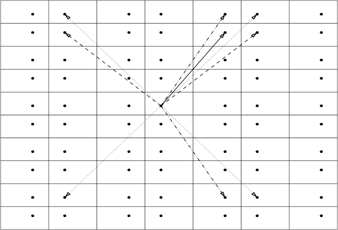
FIG. 6.: Once diffracting orbits for a typical scatterer location. The solid line represents the ($1,3$) odd-odd orbit, the dashed lines represent two of the even-odd ($2,3$) orbits, the dashed-dotted lines represent the odd-even ($1,4$) orbits and the dotted lines represents the even-even ($2,4$) orbits.

The four orbits in Fig. 6 that are in the first quadrant have all $\mu=1$, this notation is introduced since orbits in different quadrants generally have different lengths. Alternatively one can denote orbits using negative values of their index. The value of $\mu$ (see (A19) and (A30)) thus determines the signs (of $\delta_{x}$ and $\delta_{y}$) in the formulas for the lengths of the orbits. The dashed line orbit in the second quadrant in Fig. 6 is also a ($2,3$) orbits but with $\mu=2$. Its length is equal to the length of the ($2,3$) orbit with $\mu=1$. This results from the fact these orbits are related by time reversal. The other ($2,3$) orbits ($\mu=3,4$) which are not shown have the same length which differs from that of the $\mu=1,2$ orbits. This situation is typical to all even-odd and odd-even orbits (the latter have $\mu=1,4$ and are marked by dotted dashed lines in Fig. 6). The lengths of odd-odd orbits are different for different $\mu$ (these orbits are their own time reversals). The lengths of even-even orbits, marked by the dotted lines in Fig. 6, do not depend on $\mu$ and are the same as the lengths of periodic orbits.

For this reason the contribution of the even-even diffracting orbits with a single diffraction combined with one of the periodic orbits is identical to the one obtained when the scatterer is in the center and reduces to $K^{(1,e)}(\tau)$ of (16). Also the other contributions to the form factor are simply related to the ones found if the scatterer is at the center. For odd-even and even-odd $(N_{j},M_{j})$ the lengths are divided into two degenerate lengths and therefore their amplitude is $A_{j}^{(1)}/2$ (the sums over $\mu$ in (A30) consists of two pairs of identical terms) and their density is $2\rho(l_{j})$ (see (10) and (15)). The reason is that the number of orbits of each length is reduced by a factor of $2$ and the number of values of lengths in some interval increases by a factor of $2$. Since the form factor is proportional to $|A_{j}|^{2}$ and to $\rho(l_{j})$ the resulting contributions to the form factor are $\frac{1}{2}K^{(1,o-e)}(\tau)=\frac{1}{2}K^{(1,e-o)}(\tau)=\frac{|D|^{2}\tau^{2}}{8}$ (see (18)). For similar considerations (all terms in the sum over $\mu$ in (A30) are different) for the odd-odd orbits the amplitude is $\frac{1}{4}A_{j}^{(1)}$ and the density is $4\rho(l_{j})$ leading to the contribution $\frac{1}{4}K^{(1,o-o)}(\tau)=\frac{1}{16}|D|^{2}\tau^{2}$ to the form factor. The contribution to the form factor corresponding to (19) is

$$K^{(1,o)}(\tau)=\frac{5}{16}|D|^{2}\tau^{2}.$$ (61)

Therefore if the scatterer is located at a typical point the total contribution to the form factor, resulting from periodic orbits and once diffracting orbits corresponding to (20) is

$$K^{(1)}(\tau)=1+\Im D\tau+\frac{9}{16}|D|^{2}\tau^{2}.$$ (62)

We turn now to look for the saddle manifold when the scatterer is at a typical position $(a_{x}\delta_{x},a_{y}\delta_{y})$. In order to find a saddle manifold one expands the length of the diffracting segments as was done in (23). Since the shifts are of order of unity they are combined with $\delta N$ or $\delta M$ by defining

$$\delta\tilde{N_{j}} =\delta N_{j}\pm\delta_{x}$$ (63)

$$\delta\tilde{M_{j}} =\delta M_{j}\pm\delta_{y}.$$ (64)

The appropriate sign is the sign that appears in the length that is expanded. Using these definitions the rest of the calculation is identical to the one performed for the scatterer at the center except that the expansion is done with respect to $\delta\tilde{N},\delta\tilde{M}$. The condition (29) is replaced by

$$\delta\tilde{N_{j_{1}}} =-\delta\tilde{N_{j_{2}}}$$ (65)

$$\delta\tilde{M_{j_{1}}} =-\delta\tilde{M_{j_{2}}}.$$ (66)

Since $(\delta_{x},\delta_{y})$ are irrational this condition can be satisfied only if the signs of the shifts of both orbits are opposite and also if the condition (29) is satisfied. Note that the conditions for two diffracting orbits to be on the saddle manifold force these orbits to have the same parity. The contribution of each type of orbits to the form factor is calculated in what follows. For orbits of the odd-odd type both the shifts appear in the length, thus if the orbit $j_{1}$ has $\mu=1$ (the shifts have negative signs) then to satisfy (65) the $j_{2}$ orbit has to have $\nu=3$. Similarly, if one orbit has $\mu=2$ then the other one has to be of the $\nu=4$ type. Therefore, from the $16$ combinations that appear in (A30) only four will satisfy (65). The density of these contribution is $\frac{1}{4{\cal A}}$ since the odd-odd orbits are a quarter of all the orbits. The calculation of the contribution is exactly as was done in (36-39), however the two factors of $\frac{1}{4}$ result in

$$K^{{}^{\prime}(2,o-o)}(\tau)=-\frac{1}{16}\tau^{2}\Re D^{2}.$$ (67)

The contribution from the odd-even and even-odd orbits is similar, the only difference results from the fact that one of the shifts does not appear in the length of the orbit. This results in a degeneracy of lengths for orbits with different $\mu$. Thus if one orbit has $\mu=1$ then not only the orbits with $\nu=3$ will contribute but also the orbit with $\nu=2$ (or $\nu=4$) marked by the dashed line (dashed-dotted line) in Fig. 6 which has identical length. Therefore, there are $8$ combinations of $\mu,\nu$ that will contribute to the saddle manifold leading to

$$K^{{}^{\prime}(2,e-o)}(\tau)=K^{{}^{\prime}(2,o-e)}=-\frac{1}{8}\tau^{2}\Re D^{2}.$$ (68)

The contribution of the even-even orbits is

$$K^{{}^{\prime}(2,e-e)}(\tau)=-\frac{1}{4}\tau^{2}\Re D^{2}.$$ (69)

which is exactly as it was for a scatterer at the center. This is a result of the fact that the length of these orbits does not change when the scatterer position is changed. The sum of the non diagonal contributions of order $\tau^{2}$ is

$$K^{{}^{\prime}(2)}(\tau)=\frac{9}{16}\Re(-D^{2})\tau^{2}.$$ (70)

The computation of the $\tau^{3}$ terms is fairly similar to the case in which the scatterer is at the center of the rectangle. Therefore, only the relative factors resulting from the lifting of degeneracies of lengths will be calculated in what follows. The twice diffracting orbits are composed of two segments ${j_{1}}$, ${j_{2}}$. In the diagonal approximation each segment is summed independently. For the diagonal terms resulting from once diffracting orbits it was shown that a relative factor of $\frac{9}{16}$ is obtained in  (62) compared to (20). Since the sums over ${j_{1}}$ and ${j_{2}}$ are independent a relative factor of $\left(\frac{9}{16}\right)^{2}=\frac{81}{256}$ is obtained. The diagonal contribution of twice diffracting orbits for a scatterer at some typical location, corresponding to (42), is therefore,

$$K^{(3)}(\tau)=\frac{81}{512}|D|^{4}\tau^{3}.$$ (71)

We turn to compute the relative factor that results from relocating the scatterer from the center to a typical location for non diagonal terms of once and twice diffracting orbits. For this contribution, the saddle condition (65) is replaced by

$$\delta\tilde{N}_{j_{1}} = \delta\tilde{N}_{j_{2}}+\delta\tilde{N}_{j_{3}}$$ (72)

$$\delta\tilde{M}_{j_{1}} = \delta\tilde{M}_{j_{2}}+\delta\tilde{M}_{j_{3}}.$$ (73)

To understand the effect of the location of the scatterer the non integer part of (72) is studied. This non integer part depends on the displacements of the scatterer from the center $\delta_{x}$, $\delta_{y}$. It is convenient to discuss different parities of ${j_{1}}$ separately, giving a factor of $\frac{1}{4}$ to each case (since each case contributes a $\frac{1}{4}$ of the total contribution when the scatterer is at the center). If the orbit ${j_{1}}$ is even-even then the parity of $j_{2}$ should be equal to the one of ${j_{3}}$. This is exactly identical to the calculation of the non diagonal contribution of order $\tau^{2}$ which resulted in a relative factor of $\frac{9}{16}$ in (70) compared to (40). Therefore, the contribution when ${j_{1}}$ is even-even, is $\frac{9}{64}$ of the total term for the scatterer at the center, given by (48).

If the orbit ${j_{1}}$ is of the even-odd parity then the combinations of ${j_{2}}$ and ${j_{3}}$ that satisfy (72) are: (a) ${j_{2}}$ even-even; ${j_{3}}$ even-odd and (b) ${j_{2}}$ odd-odd; ${j_{3}}$ odd-even and also two combinations where the roles of ${j_{2}}$ and ${j_{3}}$ are interchanged. In case (a) there are $8$ combinations of $\mu_{j_{2}}$, $\mu_{j_{3}}$ that will satisfy (72) for each $\mu_{j_{1}}$ (compared to $16$ when the scatterer is at the center). Since this case (with ${j_{1}}$ even-odd) accounts for a $\frac{1}{4}$ of all contributions it results in a relative factor of $\frac{1}{4}\frac{8}{16}=\frac{1}{8}$. In case (b) there are $4$ combinations of $\mu_{j_{2}}$ and $\mu_{j_{3}}$ that satisfy (72) for each $\mu_{j_{1}}$. This results in a relative factor of $\frac{1}{16}$. The relative contribution of terms where ${j_{1}}$ is even-odd is thus given by $\frac{1}{4}\left(2\frac{1}{8}+2\frac{1}{16}\right)=\frac{3}{32}$, where the factors of $2$ result from the cases where the parities of ${j_{2}}$ and ${j_{3}}$ are interchanged. The case where ${j_{1}}$ is odd-even gives an identical contribution to the case in which ${j_{1}}$ is even-odd.

When ${j_{1}}$ is odd-odd (72) is solved if (c) ${j_{2}}$ is even-even and ${j_{3}}$ is odd-odd or if (d) ${j_{2}}$ is even-odd and ${j_{3}}$ is odd-even. There are also two additional solutions that result from interchanging the parities of ${j_{2}}$ and ${j_{3}}$. One can verify that for all the parities of ${j_{2}}$ there are $4$ such solutions for each value of $\mu_{j_{1}}$ compared to $16$ solutions when the scatterer is at the center. This results in a relative factor of $\frac{1}{4}\frac{1}{4}=\frac{1}{16}$ compared to (48).

Combining all the contributions from different parities of ${j_{1}}$ one finds that for a scatterer at a typical location the contribution of non diagonal terms from once and twice diffracting orbits is $\frac{9}{64}+2\frac{3}{32}+\frac{1}{16}=\frac{25}{64}$ relative to the case where the scatterer is at the center. Therefore using (48) one finds

$$K^{{}^{\prime}(3a)}(\tau)=\frac{25}{32}|D|^{2}\Im D\tau^{3}.$$ (74)

The contributions from non diagonal terms of periodic orbits and orbits with three diffractions should satisfy the condition

$$\sum_{i=1}^{3}\delta\tilde{N}_{j_{i}} = 0$$ (75)

$$\sum_{i=1}^{3}\delta\tilde{M}_{j_{i}} = 0$$ (76)

corresponding to (65). The non integer part of this condition behaves exactly in the same way as the non integer part of (72). This is true since both signs of the displacements always appear. This results in the fact that the factors relative to the case where the scatterer is at the center are equal for both of these terms. Therefore using (56) one finds

$$K^{{}^{\prime}(3b)}(\tau)=-\frac{25}{96}\Im D^{3}\tau^{3}.$$ (77)

Adding all the contributions (62), (70), (71), (74) and (77) leads to the form factor for a typical position of the scatterer

$$K(\tau)=1+\Im D\tau+\frac{9}{16}|D|^{2}\tau^{2}+\frac{9}{16}\Re(-D^{2})\tau^{2}+\frac{81}{512}|D|^{4}\tau^{3}+\frac{25}{32}|D|^{2}\Im D\tau^{3}-\frac{25}{96}\Im D^{3}\tau^{3}+O(\tau^{4}).$$ (78)

The optical theorem (58) and (59) can be used to obtain

$$K(\tau)=1-\frac{|D|^{2}}{4}\tau+\frac{9}{128}|D|^{4}\tau^{2}+\frac{81}{512}|D|^{4}\tau^{3}-\frac{25}{1536}|D|^{6}\tau^{3}+O(\tau^{4}).$$ (79)

This form factor has the same qualitative features of the form factor (60), it is $1$ for $\tau=0$ and decreases linearly for small $\tau$. See the comment following (60).

III A Model of an Integrable Billiard with a Point Scatterer

An easily solvable model is that of a point interaction [40, 41]. This interaction is the self-adjoint extension of a Hamiltonian where a point is removed from the domain. It can be viewed as formally represented by a $\delta$-function potential. The influence of such an interaction on the spectral statistics was first investigated by Šeba [11]. The system that was investigated was the rectangular billiard with a point interaction, and the spectral statistics were found to differ from Poisson statistics when the point scatterer is added. The spectral statistics of this system and of similar systems were the subject of many works [13, 36, 38, 42, 43, 44, 45, 46, 47, 48]. Since the energy levels of this system are obtained from the zeroes of a function (as will be explained in the following) it is possible to compute a large number of levels and thus also the form factor with considerable accuracy. Therefore, we use the rectangular billiard with a point scatterer to obtain numerically the form factor and compare it to the predictions of the analytical theory, presented in the previous section.

Point interactions are useful since the Green’s function of the problem $G_{\xi}(z;{\bf x},{\bf x^{\prime}})$ can be expressed by the Green’s functions of the problem in absence of the scatterer $G(z;{\bf x},{\bf x^{\prime}})$ [49]

$$G_{\xi}(z;{\bf x},{\bf x^{\prime}})=G(z;{\bf x},{\bf x^{\prime}})+T(z,\xi)G(z;{\bf x},{\bf x}_{0})G(z;{\bf x}_{0},{\bf x^{\prime}})$$ (80)

where $\xi$ is the self adjoint parameter that is related to the interaction strength, ${\bf x}_{0}$ is the scatterer location and $\Im\sqrt{z}>0$. $T$ is the on shell transition matrix and it is given by

$$T(z,\xi)=\left(e^{i\xi}\!-\!1\right)\!\left[(\Lambda i\!-\!z)\int\!dyG(z;{\bf y},{\bf x}_{0})G(\Lambda i;{\bf y},{\bf x}_{0})+e^{i\xi}(\Lambda i\!+\!z)\int\!dyG(z;{\bf y},{\bf x}_{0})G(-\Lambda i;{\bf y},{\bf x}_{0})\right]^{-1}.$$ (81)

$\Lambda$ is an energy scale usually set to be unity, since there is only one parameter in the problem which is the interaction strength. The point scatterer is characterized by the self-adjoint parameter $\xi$, while $T$ is independent of angles, resulting in s-wave scattering. The energy levels of the perturbed system are the poles of the resolvent, and if they do not coincide with the eigenvalues of the unperturbed system they are also the poles of the transition matrix $T$. The unperturbed Green’s function of the rectangular billiard is given by

$$G(z;{\bf x},{\bf x^{\prime}})=\sum_{n=1}^{\infty}\frac{\psi_{n}({\bf x})\psi_{n}({\bf x^{\prime}})}{z-E_{n}}$$ (82)

where $\psi_{n}$ and $E_{n}$ are the eigenfunctions and eigenvalues of the billiard. Substituting  (82) into (81) leads to the equation for the energy levels of the perturbed problem

$$\left(\frac{\sin\xi}{1-\cos\xi}\right)\sum_{n}\psi_{n}^{2}({\bf x}_{0})\frac{\Lambda}{\Lambda^{2}+E_{n}^{2}}-\sum_{n}\psi_{n}^{2}({\bf x}_{0})\left[\frac{1}{z-E_{n}}+\frac{E_{n}}{E_{n}^{2}+\Lambda^{2}}\right]=0.$$ (83)

In the geometrical theory of diffraction used in the previous section the effect of the scatterer that is located in the billiard was expressed by the diffraction constant $D$ that determines the scattering in free space. The diffraction constant in free space is the $T$ matrix (81) if $G(z;{\bf x},{\bf x^{\prime}})$ is the Green’s function in free space. It was calculated in App. B leading to

$$D(z)=\frac{2\pi}{-\frac{1}{2}\ln\left(\frac{z}{\Lambda}\right)+\frac{\pi}{4}\frac{\sin\xi_{1}}{1-\cos\xi_{1}}+i\frac{\pi}{2}}.$$ (84)

The self adjoint extension parameter in free space is $\xi_{1}$ and it need not to be the same as $\xi$ that was used for the bound problem (83). The reason is that the self adjoint extensions depend not only on the scatterer but also on the boundary conditions. The general relation between extensions of different problems is unexplored to the best of our knowledge, however, a connection can be made in the case that is considered here.

The energy scale associated with the scatterer is $\Lambda$. For $\Lambda\gg\Delta$ the spectrum is effectively continuous, therefore the $T$ matrix of the bound problem is approximately the diffraction constant of the unbound problem, and also the self adjoint extension parameters $\xi$ and $\xi_{1}$ should be approximately equal. Another way to establish this correspondence is to compare length scales. The length scale associated with the scatterer is $1/\sqrt{\Lambda}$ and the condition $\Lambda\gg\Delta$ is that $1/\sqrt{\Lambda}\ll\sqrt{\cal A}$ where ${\cal A}$ is the area of the billiard. The condition is that the length associated with the scatterer is much smaller then the dimensions of the billiard. This is also the condition for the validity of the semiclassical geometrical theory of diffraction used in the previous section. The scattering is strongest ($|D|^{2}$ maximal) when $D=-4i$. The variation of $D(z)$ with $z$ is weak and therefore its value at the maximum is expected to be a good approximation for a whole energy region around the maximum. Substitution of $D=-4i$ in (60) and (79) yields:

$$K(\tau)=1-4\tau+32\tau^{2}-\frac{128}{3}\tau^{3}+O(\tau^{4})$$ (85)

when the scatterer is at the center of the rectangle and

$$K(\tau)=1-4\tau+18\tau^{2}-\frac{157}{6}\tau^{3}+O(\tau^{4})$$ (86)

when the scatterer is at some typical location.

When the scatterer is at the center of the rectangle the system has a symmetry. The (unperturbed) eigenfunctions that vanish on the scatterer remain eigenfunctions of the perturbed problem, and so are their eigenvalues. To obtain the other eigenvalues one has to use only the non-vanishing eigenfunctions in (83). These are the eigenfunctions that are even functions with respect to reflection with respect to both the $X$ and $Y$ axes that pass through the center of the rectangle. Since the value of these eigenfunctions for all eigenvalues is the same ($\psi_{n}({\bf x}=0)=\frac{2}{\sqrt{\cal A}}$) at the center of the rectangle, the resulting equation (83) is the same as for the Šeba billiard with periodic boundary conditions [13]. The spectral statistics of the Šeba billiard with periodic boundary conditions were also shown to be the same as the spectral statistics of some star graphs [36, 37]. However, (85) describes the form factor of the full spectrum. Therefore, in addition to the eigenvalues that are perturbed due to the scatterer, all of the eigenvalues that are unaffected are included in the calculation of the form factor.

The form factor of the perturbed levels is related to the form factor of the full spectrum. It is composed of the even-even eigenfunctions of the rectangle. The eigenvalues of the four different symmetry classes of the rectangle can be assumed to be uncorrelated, therefore their combined form factor is the sum of the form factors (weighted using their density) of the different symmetry classes, with $\tau$ rescaled as required by (1) and (2). Since the unperturbed levels have Poisson level statistics and since levels belonging to the four symmetry classes have the same mean density (in the semiclassical limit) the relation between the full form factor and the form factor obtained from only perturbed levels is given by

$$K_{full}(\tau)=\frac{3}{4}+\frac{1}{4}K_{per}(4\tau).$$ (87)

The perturbed form factor is exactly the form factor that was computed for the Šeba billiard with periodic boundary conditions and for star graphs. The first powers in $\tau$ of the form factor for the star graphs are given by

$$K_{per}(\tau)=1-4\tau+8\tau^{2}-\frac{8}{3}\tau^{3}+O(\tau^{4}),$$ (88)

as can be seen, for example, from equation (14) of [36] where the form factor is given up to order of $\tau^{8}$. Using (87) gives exactly the form factor (85).

IV Numerical Results

The spectral form factor is not easy to compute numerically. The form factor is a very oscillatory function of time and much averaging is needed in order to obtain its mean behavior. This requires computation of many levels, which is not always possible numerically. However, such calculations are relatively easy for the point scatterer defined in the previous section by equations (80) and (81). The eigenvalues can be calculated from (83). This equation in particularly convenient since $\sum_{n}\frac{1}{z-E_{n}}$ is monotonically decreasing when $z$ is varied between any adjacent unperturbed levels, ensuring that every level must be in an interval between two adjacent unperturbed levels $E_{n}$ and $E_{n+1}$ (unless the unperturbed wavefunctions vanish at the scatterer). To compute the energy levels numerically equation (83) is solved, for example by truncating the sums at some large $n$ and replacing the tails by integrals.

This equation is solved in some energy window. The energy scale parameter is chosen so that $\Lambda\gg\Delta$, and therefore $D$ and $\xi$ can be approximated by their values for a scatterer in free space, as discussed in the previous section. In calculation presented here $\xi$ was chosen so that $D=-4i$, resulting in maximal scattering, for $z$ in the center of the window. The other values of $D$ that were also examined, are $D=2-2i$ and $D=\frac{4}{5}(2-i)$. Since $D$ does not change much with $z$ the results can be compared with the analytical predictions obtained within the semiclassical geometrical theory of diffraction.

For a scatterer at a typical location the form factor is presented in Fig. 7.

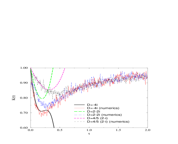
FIG. 7.: The form factor of a scatterer at a typical position, for some diffraction constants, thin lines, compared to the analytical result (79), heavy lines.

The form factor is computed from energy levels between $20000$ and $40000$. The mean level spacing is $\Delta=1$ while $\Lambda=1000$. To smooth the form factor an ensemble average over $20$ systems was performed. The aspect-ratio of each systems was taken as a random number between $1/2$ and $1$. Additional smoothing was performed by averaging the results found for $4$ consecutive values of $\tau$. The position of the scatterer was also chosen at random, but it was the same position for all ensembles of aspect ratios. Similar results were found for several other scatterer positions. The agreement between the numerical results and the theoretical prediction (79) is good at short times, where the expansion truncated at a low order is a good approximation.

For the scatterer at the center (${\bf x}_{0}={\bf 0}$) only levels with eigenfunctions that are symmetric with respect to the $X$ and $Y$ axes are perturbed by the scatterer as is clear from (83). Based on the assumption that the spectra of the various symmetry classes of levels are uncorrelated (87) was derived. To test it the form factor of the full spectrum and of the levels which are affected by the scatterer were calculated. These are shown in Fig. 8. The calculation is done for parameters similar to the ones used in the case where the scatterer is not at the center, and an averaging over $70$ systems is performed here, while the energy range considered was $60000-80000$.

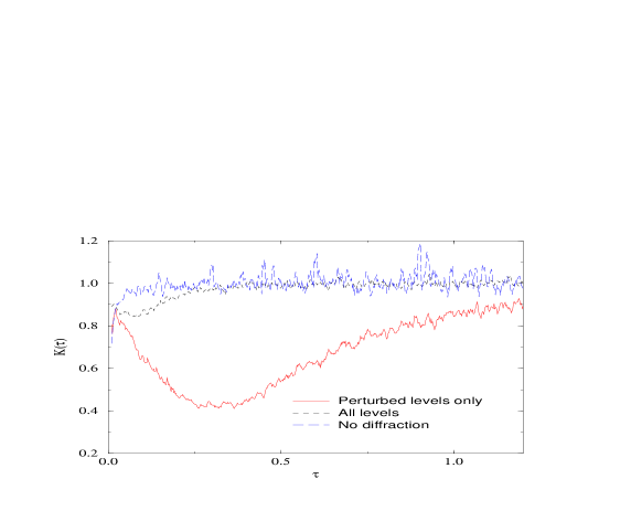
FIG. 8.: The form factor of a scatterer at the center (${\bf x}_{0}={\bf 0}$), for only perturbed levels as well as the full form factor

The form factor of the rectangular billiard was included for comparison, demonstrating that at short times all form factors deviate from $1$. This deviation is due to the fact that one examines times of the order of the period of the shortest orbits and there are not enough orbits that contribute to the form factor for such times. In order to demonstrate it, the form factor of the rectangle was calculated from the exact energy levels in the same way as the form factors with diffraction. The result is shown in Fig. 8 and this form factor is also found to deviate from $1$ at short times. The form factor calculated from all levels and the scaled form factor obtained from the perturbed levels with the help of (87) are compared to the analytical result (85) in Fig. 9.

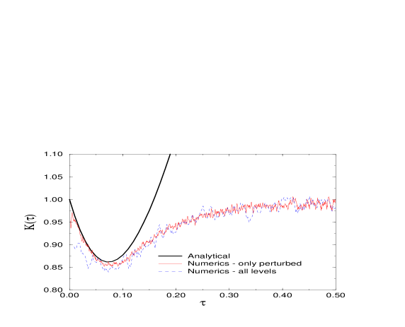
FIG. 9.: The form factor for the scatterer at the center (${\bf x}_{0}={\bf 0}$) compared to the scaled form factor calculated from perturbed levels by (87) and the analytical result (85)

It is clear that the symmetry argument (87) is valid. The scaled form factor is indeed the same as the one that is obtained from the full spectrum. Both slightly deviate from the analytical prediction (85). The deviation at short times of the full form factor is due to the fact that there are not enough relevant short orbits as was discussed earlier, and at these times the scaled form factor is probably more accurate. Since the periodic orbits prediction is in agreement with the form factor studied in [13, 36, 37] (that is exact) the deviation probably results from the numerical solution, or of the fact that the energy is not high enough.

The agreement between the analytical results obtained in Sec. II and the numerical results of the model of the point scatterer outlined in Sec. III was found for $\Lambda\gg\Delta$, where for the point scatterer the values of $\xi$ and $D$ of a scatterer in free space were used. The requirement $\Lambda\gg\Delta$ is essential for this agreement. For $\Lambda\approx\Delta$ if one uses $D=-4i$ and the corresponding values of the self adjoint extension parameter $\xi$, found for the scatterer in free space, the effect of the point scatterer on the spectrum of the bounded system is even not maximal (as is the case when $\Lambda\gg\Delta$) and clearly there is no agreement with predictions of Sec. II for these values of $\Lambda$ and $D$.

V Scattering From a Localized Potential

So far it was assumed that the diffraction constant is given. In this section the diffraction constant for a given potential, which is localized around some point, is calculated. Consider a potential which is assumed to have a length scale $a$ such that

$$U({\bf r})=\frac{1}{a^{2}}f\left(\frac{{\bf r}}{a}\right)$$ (89)

where $f({\bf y})$ is small for ${\bf y}$ that is large compared to unity. The scattering from such a potential at energies for which the wave number $k$ satisfies, $ka\ll 1$, is studied in what follows.

The diffraction constant is the on shell matrix element of the ${\bf T}$ matrix

$$D(\theta^{\prime},\theta)=\langle{\bf k}|{\bf T}(E)|{\bf q}\rangle$$ (90)

where ${\bf k}$ is the outgoing momentum (in direction $\theta^{\prime}$) and ${\bf q}$ is the incoming momentum (in the direction $\theta$). The energies of the incoming and outgoing waves are equal, that is

$$k=q=\sqrt{E}$$ (91)

(in units $\hbar=1$ and $m=\frac{1}{2}$ used in the paper). In order to compute the diffraction constant it is convenient to start from the Lippman-Schwinger equation for the ${\bf T}$ matrix

$${\bf T}(E)=g{\bf U}+g{\bf UG}(E){\bf T}(E)$$ (92)

where ${\bf G}(E)$ is the Green’s function for free propagation at energy $E$ and $g$ is an expansion parameter which will be set to unity at the end of the calculation. One might be tempted to compute the on shell matrix elements of ${\bf T}$ using the Born approximation which is obtained by iterating equation (92)

$$\langle{\bf k}|{\bf T}(E)|{\bf q}\rangle=g\langle{\bf k}|{\bf U}|{\bf q}\rangle+g^{2}\langle{\bf k}|{\bf UGU}|{\bf q}\rangle+g^{3}\langle{\bf k}|{\bf UGUGU}|{\bf q}\rangle+\cdots$$ (93)

However, in the limit $ka\rightarrow 0$ the Green’s function diverges as $\ln ka$ and therefore the Born series diverges.

A method which behaves regularly at low energies ($ka\ll 1$) was developed by Noyce [50]. In this method the scattering in the forward direction (another chosen direction can also be used) is in some sense resummed. In two dimensions this method was used to describe low energy bound states [51] and low energy scattering [52]. The Noyce method is derived in the following. The ${\bf T}$ matrix is written as a product of the diagonal matrix element times a function of the incoming and outgoing momenta,

$$\langle{\bf k}|{\bf T}|{\bf q}\rangle=h({\bf k},{\bf q})\langle{\bf q}|{\bf T}|{\bf q}\rangle.$$ (94)

Taking the diagonal matrix elements of the Lippmann-Schwinger equation (92) leads to

$$\langle{\bf q}|{\bf T}|{\bf q}\rangle\left(1-g\frac{1}{(2\pi)^{2}}\int d^{2}k_{1}\frac{\langle{\bf q}|{\bf U}|{\bf k}_{1}\rangle h({\bf k}_{1},{\bf q})}{E+i\epsilon-k_{1}^{2}}\right)=g\langle{\bf q}|{\bf U}|{\bf q}\rangle,$$ (95)

where the Green’s function in the momentum representation is

$$G(E;{\bf k}_{1},{\bf k}_{2})=\frac{(2\pi)^{2}\delta\left({\bf k}_{1}-{\bf k}_{2}\right)}{E-k_{1}^{2}+i\epsilon}.$$ (96)

Note that ${\bf k}_{1}$ is not on the energy shell.

Using (95) in the non diagonal matrix elements of (92) leads to an integral equation for $h$:

$$h({\bf k}_{1},{\bf q}) = \frac{\langle{\bf k}_{1}|{\bf U}|{\bf q}\rangle}{\langle{\bf q}|{\bf U}|{\bf q}\rangle}+g\frac{1}{(2\pi)^{2}}\int d^{2}k_{2}\left(\langle{\bf k}_{1}|{\bf U}|{\bf k}_{2}\rangle-\frac{\langle{\bf k}_{1}|{\bf U}|{\bf q}\rangle\langle{\bf q}|{\bf U}|{\bf k}_{2}\rangle}{\langle{\bf q}|{\bf U}|{\bf q}\rangle}\right)$$ (98)

$$\times\frac{1}{E+i\epsilon-k_{2}^{2}}h({\bf k}_{2},{\bf q}).$$

This equation can be iterated resulting in an expansion of $h$ in powers of $g$. Therefore with the help of (94) and (95) the ${\bf T}$ matrix can be written in the form

$$\langle{\bf k}|{\bf T}|{\bf q}\rangle=\frac{gh({\bf k},{\bf q})\langle{\bf q}|{\bf U}|{\bf q}\rangle}{D_{g}({\bf q})}.$$ (99)

Both $h({\bf k},{\bf q})$ and the denominator $D_{g}({\bf q})$ can be expanded in powers of $g$ as

$$h({\bf k},{\bf q}) = \frac{\langle{\bf k}|{\bf U}|{\bf q}\rangle}{\langle{\bf q}|{\bf U}|{\bf q}\rangle}+g\left(\frac{\langle{\bf k}|{\bf UGU}|{\bf q}\rangle}{\langle{\bf q}|{\bf U}|{\bf q}\rangle}-\frac{\langle{\bf k}|{\bf U}|{\bf q}\rangle\langle{\bf q}|{\bf UGU}|{\bf q}\rangle}{\langle{\bf q}|{\bf U}|{\bf q}\rangle^{2}}\right)$$ (102)

$$+g^{2}\left(\frac{\langle{\bf k}|{\bf UGUGU}|{\bf q}\rangle}{\langle{\bf q}|{\bf U}|{\bf q}\rangle}-\frac{\langle{\bf k}|{\bf UGU}|{\bf q}\rangle\langle{\bf q}|{\bf UGU}|{\bf q}\rangle}{\langle{\bf q}|{\bf U}|{\bf q}\rangle^{2}}\right.$$

$$\left.-\frac{\langle{\bf k}|{\bf U}|{\bf q}\rangle\langle{\bf q}|{\bf UGUGU}|{\bf q}\rangle}{\langle{\bf q}|{\bf U}|{\bf q}\rangle^{2}}+\frac{\langle{\bf k}|{\bf U}|{\bf q}\rangle\langle{\bf q}|{\bf UGU}|{\bf q}\rangle^{2}}{\langle{\bf q}|{\bf U}|{\bf q}\rangle^{3}}\right)+\cdots$$

and

$$D_{g}({\bf q}) = 1-g\frac{\langle{\bf q}|{\bf UGU}|{\bf q}\rangle}{\langle{\bf q}|{\bf U}|{\bf q}\rangle}-g^{2}\left(\frac{\langle{\bf q}|{\bf UGUGU}|{\bf q}\rangle}{\langle{\bf q}|{\bf U}|{\bf q}\rangle}-\frac{\langle{\bf q}|{\bf UGU}|{\bf q}\rangle^{2}}{\langle{\bf q}|{\bf U}|{\bf q}\rangle^{2}}\right)$$ (105)

$$-g^{3}\left(\frac{\langle{\bf q}|{\bf UGUGUGU}|{\bf q}\rangle}{\langle{\bf q}|{\bf U}|{\bf q}\rangle}-2\frac{\langle{\bf q}|{\bf UGU}|{\bf q}\rangle\langle{\bf q}|{\bf UGUGU}|{\bf q}\rangle}{\langle{\bf q}|{\bf U}|{\bf q}\rangle^{2}}\right.$$

$$\left.+\frac{\langle{\bf q}|{\bf UGU}|{\bf q}\rangle^{3}}{\langle{\bf q}|{\bf U}|{\bf q}\rangle^{3}}\right)+\cdots$$

While the expansions for $h({\bf k},{\bf q})$ and $D_{g}({\bf q})$ seem to be complicated they are actually composed of all the ways to break the matrix elements, containing chains of the form ${\bf UGUG\cdots UGU}$ with several Green’s functions, to products of smaller elements with less Green functions. Each order of $g$ consists of terms with the same number of Green’s functions in it, and when an element is broken into a product an extra factor of $\frac{-1}{\langle{\bf q}|{\bf U}|{\bf q}\rangle}$ is added. In the expansion for $D_{g}({\bf q})$ all factors contain at least one Green’s function but in the expansion for $h({\bf k},{\bf q})$ factors of the type $\langle{\bf k}|{\bf U}|{\bf q}\rangle$ appear. Consequently the $g^{N}$ term for $h({\bf k},{\bf q})$ can be explicitly written. It includes $2^{N}$ terms (and $2^{N-1}$ terms for $D_{g}({\bf q})$, some of which may be identical). Note that $\frac{1}{D_{g}({\bf q})}$ can be expanded in powers of $g$ leading back to the Born series (93).

To compute the diffraction constant the matrix elements are computed and the length scale $a$ of the potential is scaled out. For example

$$\langle{\bf k}|{\bf UGU}|{\bf q}\rangle = \int d^{2}r_{1}d^{2}r_{2}e^{-i{\bf k\cdot r}_{1}}U({\bf r}_{1})G_{0}({\bf r}_{1},{\bf r}_{2})U({\bf r}_{2})e^{i{\bf q\cdot r}_{2}}$$ (106)

$$= \int d^{2}y_{1}d^{2}y_{2}e^{-ia{\bf k\cdot y}_{1}}f({\bf y}_{1})G_{0}(ka;{\bf y}_{1},{\bf y}_{2})f({\bf y}_{2})e^{ia{\bf q\cdot y}_{2}}$$ (107)

where ${\bf y}_{i}=\frac{{\bf r}_{i}}{a}$ and (89) was used and $G_{0}$ is the free Green’s function in the position representation, namely $G_{0}({\bf r}_{1},{\bf r}_{2})\equiv\langle{\bf r}_{1}|{\bf G}(E)|{\bf r}_{2}\rangle\equiv G_{0}(ka;{\bf y}_{1},{\bf y}_{2})$, where $k=\sqrt{E}$. These matrix elements are expanded for $ka\ll 1$ keeping terms of order $k^{2}a^{2}$. Then the series in the parameter $g$ is summed.

Both the exponentials $\langle{\bf k}|{\bf r}\rangle=e^{-i{\bf k\cdot r}}$ and the Green’s function should be expanded to the same order. In the limit of small $ka$ one finds

$$G_{0}(ka;{\bf y}_{1},{\bf y}_{2})=-\frac{i}{4}H_{0}^{(1)}(ka|{\bf y}_{-}{\bf y}_{2}|)\simeq d_{1}+\phi({\bf y}_{1},{\bf y}_{2})-\frac{k^{2}a^{2}}{4}|{\bf y}_{1}-{\bf y}_{2}|^{2}\left(d_{1}-\frac{1}{2\pi}+\phi({\bf y}_{1},{\bf y}_{2})\right)$$ (108)

where

$$d_{1}=\frac{1}{2\pi}\left(\gamma+\ln\left(\frac{ka}{2}\right)\right)-\frac{i}{4}$$ (109)

and

$$\phi({\bf y}_{1},{\bf y}_{2})=\frac{1}{2\pi}\ln|{\bf y}_{1}-{\bf y}_{2}|$$ (110)

while $\gamma$ is Euler’s constant. The leading order part of the Green’s function which is coordinate independent is $d_{1}$ and, as was mentioned earlier, it diverges logarithmically when $ka\rightarrow 0$. In App. C it is shown that in many of the terms to be computed this constant part will be canceled. This is the advantage of the Noyce method [50] compared to the Born expansion for the present problem.

Calculations presented in App. C lead to the asymptotic expression for the angular dependence of the diffraction constant

$$D(\theta^{\prime},\theta) \simeq \frac{gV_{0}}{V(g)-gV_{0}d_{1}+k^{2}a^{2}Q(g)}\left[1-k^{2}a^{2}M_{0}\right.+i\frac{ka}{2}V(g)\left\{\left(e^{i\theta}-e^{i\theta^{\prime}}\right)\frac{\alpha(g)}{V_{0}}+c.c\right\}$$ (111)

$$- \frac{k^{2}a^{2}}{8}\left\{V(g)\left(e^{2i\theta}+e^{2i\theta^{\prime}}\right)\frac{\sigma(g)}{V_{0}}+c.c.\right\}+\frac{k^{2}a^{2}}{4}\left[M_{++}e^{i(\theta+\theta^{\prime})}+M_{+-}e^{i(-\theta+\theta^{\prime})}\right.$$ (112)

$$+ \left.\left.M_{-+}e^{i(\theta-\theta^{\prime})}+M_{--}e^{-i(\theta+\theta^{\prime})}\right]\right]$$ (113)

where $c.c.$ stands for complex conjugate,

$$Q(g)\equiv\frac{1}{4}V^{2}(g)\sum_{k=1}^{\infty}g^{k}\frac{{{\cal L}_{k}}}{V_{0}}+\frac{1}{2}\left(V(g)-\frac{gV_{0}}{2\pi}\right)V(g)\left(\frac{\delta(g)}{V_{0}}-V(g)\frac{|\alpha(g)|^{2}}{V_{0}^{2}}\right),$$ (114)

$$M_{0}=\frac{V^{2}(g)}{2}\frac{|\alpha(g)|^{2}}{V_{0}^{2}}$$ (115)

and

$$M_{++} = \left(V(g)-gd_{1}V_{0}\right)\frac{\mu^{(++)}(g)}{V_{0}}+V(g)gd_{1}V_{0}\frac{\alpha^{2}(g)}{V_{0}^{2}}$$ (116)

$$M_{+-} = \left(V(g)-gd_{1}V_{0}\right)\frac{\mu^{(+-)}(g)}{V_{0}}+V(g)gd_{1}V_{0}\frac{|\alpha(g)|^{2}}{V_{0}^{2}}$$ (117)

$$M_{-+} = \left(V(g)-gd_{1}V_{0}\right)\frac{\mu^{(-+)}(g)}{V_{0}}+V(g)gd_{1}V_{0}\frac{|\alpha(g)|^{2}}{V_{0}^{2}}$$ (118)

$$M_{--} = \left(V(g)-gd_{1}V_{0}\right)\frac{\mu^{(--)}(g)}{V_{0}}+V(g)gd_{1}V_{0}\frac{(\alpha^{*}(g))^{2}}{V_{0}^{2}}.$$ (119)

The constants $V_{0},V(g),\mu^{(a,b)}(g),\alpha(g),\sigma(g),\delta(g)$, and ${\cal L}_{k}$ are angle and energy independent and are given by a series of integrals over the potential. They are defined in (C7),(C21), and (C29)-(C49).

Equation (111) is the main result of this section. It provides the functional form of the diffraction constant for $ka\ll 1$. It also gives a recipe for the computation of the coefficients of the angle dependent factors as sums of certain integrals involving the potential (89). The physical scattering constant is obtained when $g=1$ is substituted in (111). It is of interest to note that the simple dependence on the angles $\theta$ and $\theta^{\prime}$ is expected since formally it should be the same dependence as in the Born series (93) which is also simple. This diffraction constant will be used in Sec. VI for the calculation of the effects of angular dependence on the form factor.

Finally, one can verify that the diffraction constant (111) satisfies the optical theorem

$$\Im D(\theta,\theta)=-\frac{1}{8\pi}\int_{0}^{2\pi}d\theta^{\prime}\;\left|D(\theta^{\prime},\theta)\right|^{2}$$ (120)

up to order $k^{2}a^{2}$.

VI The effect of Angular Dependence on the Form Factor

In this section the form factor resulting of angle dependent diffraction is calculated to order $\tau^{2}$. The complicated parts of the calculation are not related to the dependence on the angles but rather to the contribution from non diagonal terms that were calculated in Sec. II, therefore this calculation will not be repeated here, and only the modifications needed to describe angle dependent diffraction constants will be presented.

Since the diffraction constant depends on angles, the density of diffracting orbits of length $l$ and outgoing direction $\theta$ is needed (the incoming direction depends on the outgoing direction, via (A18)). For simplicity consider first the case where the scatterer is at the center. Instead of orbits that leave the scatterer, hit the walls, and return to the scatterer it is possible to examine orbits which connect the scatterer to one of its images, when the plane is tiled with rectangles, as described in detail in App. A. These orbits have the same length and the same outgoing directions as the diffracting orbits. To compute the (averaged) density of such orbits the number of orbits with lengths in the range $(l-\frac{\delta l}{2},l+\frac{\delta l}{2})$ and outgoing directions in the range $(\theta-\frac{\delta\theta}{2},\theta+\frac{\delta\theta}{2})$ is estimated. The area of this domain is $l\delta\theta\delta l$. When computing the form factor, in the semiclassical limit, the lengths of orbits that contribute scales as $k$. There is a natural width $\delta l$ which results from the averaging in (2) and is taken such that $1\ll\delta l\ll l$. Therefore, for any small but finite $\delta\theta$ the area $l\delta\theta\delta l$ is large in the semiclassical limit. The number of orbits (of a each type) in such area is given by $\frac{l}{4{\cal A}}\delta\theta\delta l$. If the diffraction constant depends slowly on the angles, that is, its value changes considerably only when the angles change by $\delta\theta\sim 1$ (namely $O(k^{0})$) then the sums over diffracting orbits can be replaced by integrals with the density

$$\tilde{\rho}(\l,\theta)=\frac{l}{4{\cal A}}.$$ (121)

On this scale the angles of diffracting orbits are distributed uniformly. Note that if the diffraction constant is angle independent one can integrate (121) over $\theta$ in the interval $(0,\frac{\pi}{2})$ and obtain (15). As a result the form factor for an angle dependent diffraction constant can be computed if instead of the constant $D$ of Sec. II one uses $D(\theta^{\prime},\theta)$ of (111) with $g=1$ with appropriate averages on angles. These averages depend on the type of the diffracting orbits that contribute and are computed in the following.

A Scatterer at the center

To compute the contributions to the form factor each type of orbits should be considered separately. This results from the fact that the incoming direction is related to the outgoing direction in a different way characterized by the parity and by the indices $\mu$ and $\nu$ of App. A, where it is explicitly given by (A18). First the diagonal contribution from diffracting orbits is computed and later the non diagonal contributions from twice diffracting orbits and periodic orbits will be computed.

First consider the contribution of the even-even orbits following the lines of the calculation leading to (16) of Sec. II. This is the contribution of forward diffracting orbits. For these orbits the incoming direction is the same as the outgoing direction. The index $\mu$ of (A30) specifies the quadrant of the angle. In Sec. II the factor resulting of summation over $\mu$ was included in the amplitude but for the angle dependent $D(\theta^{\prime},\theta)$ the averaging over angles is performed with the help of the density (121). The summation over $\mu$ results in extension of the integration interval from $(0,\frac{\pi}{2})$ to $(0,2\pi)$. When the scatterer is at the center orbits with different $\mu$ (but with the same index ${\bf N}_{1},{\bf N}_{2}$) have identical lengths. Since

$$\Im\frac{2}{\pi}\int_{0}^{\frac{\pi}{2}}\!d\theta\;\frac{1}{4}\left[{D(\theta,\theta)+D(\pi\!-\!\theta,\pi\!-\!\theta)+D(\pi\!+\!\theta,\pi\!+\!\theta)+D(2\pi\!-\!\theta,2\pi\!-\!\theta)}\right]=\frac{1}{2\pi}\Im\int_{0}^{2\pi}d\theta\;D(\theta,\theta)$$ (122)

and

$$\frac{2}{\pi}\int_{0}^{\frac{\pi}{2}}d\theta\;\frac{1}{16}\left|{D(\theta,\theta)+D(\pi-\theta,\pi-\theta)+D(\pi+\theta,\pi+\theta)+D(2\pi-\theta,2\pi-\theta)}\right|^{2}$$ (123)

$$=\frac{1}{8\pi}\int_{0}^{2\pi}d\theta\;D^{*}(\theta,\theta)\left[D(\theta,\theta)+D(\pi-\theta,\pi-\theta)+D(\pi+\theta,\pi+\theta)+D(2\pi-\theta,2\pi-\theta)\right]$$ (124)

the contribution of even-even orbits, that are the forward diffracting orbits, to the form factor is given by

$$K^{(1,e)}(\tau) = 1+\frac{\tau}{2\pi}\Im\int_{0}^{2\pi}d\theta\;D(\theta,\theta)$$ (125)

$$+ \frac{\tau^{2}}{32\pi}\int_{0}^{2\pi}d\theta\;D^{*}(\theta,\theta)\left[D(\theta,\theta)+D(\pi-\theta,\pi-\theta)+D(\pi+\theta,\pi+\theta)+D(2\pi-\theta,2\pi-\theta)\right].$$ (126)

This contribution corresponds to (16) of Sec. II. The diagonal contributions from the other types of diffracting orbits are computed in a similar manner and presented in App. D 1. Substitution of the diffraction constant (111) in the diagonal contribution (D7) leads to

$$K^{(1)}(\tau)=1-\frac{1}{4}|C|^{2}\tau+|C|^{2}C^{\prime}\tau^{2}$$ (127)

where

$$C\equiv\frac{V_{0}}{V(1)-V_{0}d_{1}+k^{2}a^{2}Q(1)}$$ (128)

and

$$C^{\prime}\equiv 1-k^{2}a^{2}V^{2}(1)\left|\frac{\alpha(1)}{V_{0}}\right|^{2}.$$ (129)

See (109), (114), (C7), (C22), and (C49) for the definitions of the various quantities used in (128) and (129).

An additional non diagonal contribution results from orbits which have almost identical lengths. At order $\tau^{2}$ such a contribution results from combinations of twice diffracting orbits and periodic orbits. For angle independent scattering this contribution was computed in Sec. II (see (21-40) there). The modifications which result from the angle dependence are computed in App. D 2 leading to (D29) that yields

$$K^{{}^{\prime}(2)}(\tau)=-(\Re C^{2})C^{\prime}\tau^{2}$$ (130)

where $C$ and $C^{\prime}$ are defined by (128) and (129). To obtain the form factor of an angle dependent scatterer located at the center of a rectangular billiard, to order $\tau^{2}$, equations (127) and (130) are summed resulting in

$$K(\tau)=1-\frac{1}{4}|C|^{2}\tau+\frac{1}{8}|C|^{4}C^{\prime}\tau^{2}.$$ (131)

This form factor resembles the form factor (60) that was obtained for angle independent scattering. It starts at $1$ and decreases for small times until at some point it has a minimum. At larger times it rises and approaches $1$ for long times. The angle dependence just modifies the constants in front the powers of $\tau$, but these changes are of the order $k^{2}a^{2}$ and typically cannot change the sign of these coefficients.

B Scatterer at a typical position

When the scatterer is not at the center the lengths of the diffracting segments of the same parity vary and some length degeneracies are lifted, as discussed at the end of Sec. II. The form factor for an angle dependent scatterer in some typical position is calculated along the lines of the calculation of Sec. II. Only the modifications due to the angle dependence are presented. First the diagonal contribution from once diffracting orbits is computed and then the non diagonal contributions from combinations of twice diffracting orbits and periodic orbits are computed.

To compute the diagonal contribution it is convenient to separate the orbits into types determined by the number of bounces from the walls (or the parity of their index ${\bf N}_{j}$). For orbits of the even-even type the lengths of all $4$ possible segments (with different $\mu$) are identical and do not change when the scatterer changes position. Therefore their diagonal contribution is identical to the contribution that was obtained for a scatterer at the center and is given by (125). The other contributions are calculated in App. D 3 leading to

$$K^{(1)}(\tau)=1-\frac{1}{4}|C|^{2}+\frac{3}{16}|C|^{2}(\Re C_{1}^{\prime})\tau^{2}$$ (132)

where

$$C_{1}^{\prime}\equiv 3+k^{2}a^{2}\left[V(1)-V_{0}d_{1}\right]\left[\frac{\Re\mu^{(+-)}(1)}{V_{0}}-\frac{V(1)|\alpha(1)|^{2}}{V^{2}_{0}}\right]$$ (133)

and the various quantities are defined by (109), (128), (C7), (C22), and (C49). This is not the total contribution to the form factor (in order $\tau^{2}$). There is a non diagonal contribution from twice diffracting orbits and periodic orbits which is computed in App. D 4 and is described in what follows.

The non diagonal contributions are from twice diffracting orbits and periodic orbits with almost identical lengths. The condition for such combinations to contribute is given by (65). This condition ensures that the two segments of the diffracting orbit are of the same type, as it was for the scatterer at the center. The fact that the lengths of the segments might depend on the index $\mu$ was discussed following the condition (65). This discussion is also valid for angle depended scattering. As for the case where the scatterer is at the center the integral over angles can be factored out of the saddle manifold integral.

For even-even orbits the lengths do not depend upon $\mu$ and the non diagonal contribution from these orbits and periodic orbits is given by (D14). The other contributions are calculated in App. D 4 resulting in (D52) leading to

$$K^{{}^{\prime}(2)}(\tau)=-\frac{3}{16}\Re(C^{2}C_{1}^{\prime})\tau^{2},$$ (134)

where $C_{1}^{\prime}$ is given by (133). Finally summing (132) and (134) results in an expression for the form factor, correct to order $\tau^{2}$, for the case where the scatterer is at a typical position,

$$K(\tau)=1-\frac{1}{4}|C|^{2}\tau+\frac{9}{128}|C|^{4}\tau^{2}.$$ (135)

This form factor is rather similar to the one obtained for angle independent scattering (79). The angle dependence modifies the coefficients only slightly. The coefficient $C$ satisfies the optical theorem (58), therefore this form factor is identical to one obtained for an angle independent potential, with diffraction constant $C$.

VII Summary and Discussion

In this paper the form factor $K(\tau)$ was calculated for a rectangular billiard perturbed by a strong potential, that is confined to a region which is much smaller than the wavelength. In the first part (Secs. II, III and IV) a highly idealized situation of a scatterer that is confined to a point and its action is represented by the diffraction constant $D$, that is a complex number like $D=-4i$ or $D=2-2i$, was explored. The form factor $K(\tau)$ was calculated to $O(\tau^{3})$ and the results are given by (60), if the scatterer is at the center, and by (79) if it is at a typical position. These results were compared to the ones obtained numerically for various values of $D$ in Figs. 7 and 9. Reasonable agreement was found in the small $\tau$ regime, up to the minimum. The numerical calculations were performed for the Šeba billiard, that is a rectangular billiard with a $\delta$-like scatterer inside. Its $T$ matrix is (81) and the energy levels, used in the numerical calculation of the form factor, were obtained from the numerical solution of (83). This is an idealized model approximating a rectangular billiard with a strong potential that is confined to a very small region. The model is defined by the self-adjoint parameter $\xi$ and the energy scale is set by $\Lambda$. The connection with the analytical results of Sec. II is via the diffraction constant $D$ of (84), that is defined in free space. If $\Lambda\gg\Delta$, where $\Delta$ is the mean level spacing (or $1/\sqrt{\Lambda}$ is much smaller then the dimensions of the billiard), then the self-adjoint parameter $\xi_{1}$ of (84) is approximately equal to $\xi$, that is the corresponding parameter in the presence of the boundary. This condition was found to be essential. The variation of $D$ with energy is slow. For these reasons the numerical results of Figs. 7 and 9 are expected to agree with the analytical predictions of Sec. II, for small $\tau$, and indeed such agreement is found.

In the second part of the paper (Secs. V and VI) a problem with an arbitrary perturbing potential $U({\bf r})$ of (89), that is large in a small region of extension $a$, was studied. For rectangles with such potentials the diffraction constant was calculated to the order $(ka)^{2}$, where $k=2\pi/\lambda=\sqrt{E}$ is the wavenumber. The result is given by (111) with $g=1$. The angle dependent terms are of order $ka$ and $(ka)^{2}$. In the limit $(ka)^{2}\ll 1$ or $a\ll\lambda$ the diffraction constant $D(\theta^{\prime},\theta)$ is approximately independent of angles and reduces to

$$C_{0}=\frac{1}{\frac{V(1)}{V_{0}}-\frac{1}{2\pi}\left(\gamma+\ln\left(\frac{ka}{2}\right)\right)+\frac{i}{4}},$$ (136)

where $V_{0}$ and $V(g)$ are given by (C7) and (C21) while $\gamma$ is Euler’s constant. One can easily see that $C_{0}$ satisfies the optical theorem. We do not know much about the convergence of the series (C21) and (C22) for $V(g)$. Therefore $V(1)$ is assumed to be the analytic continuation from the small $g$ region. Exploration of these series for various potentials is left for further research. If the potential is such that in the $a\rightarrow 0$ limit $C_{0}$ is well defined, then in this limit it approaches the diffraction constant $D$ that was studied in the first part of the paper, taking the constant value $D$ in Sec. II and (84) in Secs. III and IV. For this to hold it is required that in the limit $a\rightarrow 0$ also

$$\frac{V(1)}{V_{0}}-\frac{1}{2\pi}\left(\gamma+\ln\left(\frac{ka}{2}\right)\right)\longrightarrow-\frac{1}{4\pi}\ln\left(\frac{k^{2}}{\Lambda}\right)+\frac{1}{8}\frac{\sin\xi_{1}}{1-\cos\xi_{1}}.$$ (137)

If the function $f({\bf y})$ of (89) is independent of $a$, then also $V(1)/V_{0}$ is independent of $a$, as is clear from (C7) and (C21). The calculations of Sec. V and App. C, leading to (111), do not require that $f$ is independent of $a$. Assume for example that $f$ factors in the form

$$f(a,{\bf y})=\bar{f}\left(\frac{a}{l_{\Lambda}}\right)f_{1}({\bf y})$$ (138)

where $f_{1}({\bf y})$ is independent of $a$, while $\bar{f}$ is independent of ${\bf y}$ and $l_{\Lambda}$ is some characteristic length scale. If $\lim_{a\rightarrow 0}\bar{f}(a/l_{\Lambda})=0$ then $\lim_{a\rightarrow 0}V(1)=1$. The factorization (138) implies

$$V_{0}=\bar{f}\left(\frac{a}{l_{\Lambda}}\right)\int d^{2}yf_{1}({\bf y}).$$ (139)

Existence of the limit (137) requires that

$$V_{0}\sim 2\pi\left[\ln\left(\frac{a}{l_{\Lambda}}\right)+\bar{f}_{0}\right]^{-1}$$ (140)

where $\bar{f}_{0}$ is a constant independent of $a$, in agreement with the scaling used in the mathematical literature ([40] p. 103). It leads to the natural identification $l_{\Lambda}^{2}=\frac{1}{\Lambda}$. Therefore $l_{\Lambda}$ is the length scale associated with the energy scale $\Lambda$ that was discussed after (84). The limit is characterized by the two parameters $\xi$ and $\Lambda$. If the factorization (138) exists, then for $a\ll\lambda$ the results obtained in the first part of the paper provide a good approximation for the ones obtained in the second one, for arbitrary but well defined potentials $U$ of (89). For any given potential $U({\bf r})$ that is concentrated in a small region, of extension $a$, one can use (111) to compute the form factor. The condition for the applicability of the semiclassical approximation combined with the geometrical theory of diffraction (GTD) is

$$a\ll\lambda\ll a_{x},~{}a_{y},$$ (141)

where $a_{x}$ and $a_{y}$ are the sides of the rectangle.

If the scatterer is at a typical position then the form factor is given by (135). Note that $C$ of Eq. (135) (defined by (128)) satisfies the optical theorem, since $Q(1)$ is real. Therefore the form factor of the angle dependent scatterer reduces (to the order $\tau^{2}$) to (79). That is, the angle dependent scattering is affecting the form factor in the same way (to the order computed here) as angle independent scattering. Therefore the angle dependence plays no role up to this order. For the scatterer at the center the situation is somewhat different. In this case, the form factor (131) should be compared with (60). There is a correction $C^{\prime}$ resulting of the angular dependence of $D(\theta^{\prime},\theta)$ given by (111). This difference is a consequence of the increased number of length degeneracies of the diffracting orbits when the scatterer is at the center compared to the situation when it is located at a typical position.

For the case where the scatterer is at a typical position, using angle dependent terms to order $(ka)^{2}$ does not change the result for the form factor, compared to the one found for the angle independent leading order. Therefore it is reasonable to assume that the results are robust and the limit $a\rightarrow 0$ describes correctly the physics of the regime $a<\lambda$. This is so although the classical dynamics (in the long time limit) are expected to be chaotic in nearly all of phase space and similar to the ones of the Sinai billiard. This improves the chances for the experimental realization of the results of the present work. Note that for $a\gg\lambda$, semiclassical theory works and the system should behave as a Sinai billiard, with level statistics given by Random Matrix Theory (RMT), in some range [7, 30].

The spectral statistics found in the present work differ from the ones of the known universality classes. It is characterized by the form factor of the type presented in Figs. 7 and 9. A characteristic feature of the form factor is that it is equal to 1 at $\tau=0$, resulting of the fact that for small $\tau$ the number of classical orbits that are scattered is small. The contribution that is first order in $\tau$ originates from the term (14), that leads to the contribution $\Im D\tau$ in (20), (57) and (78). By the optical theorem (58) it is always negative. This is expected to hold for a larger class of systems, where there is forward diffraction along periodic orbits. For $\tau\gg 1$ the form factor approaches unity because of the discreteness of the spectrum [30]. These are the physical reasons for the qualitative form of $K(\tau)$ depicted in Figs 7 and 9.

The form factor was computed when the scatterer is at the center and when it is at a typical position shifted by $(a_{x}\delta_{x},a_{y}\delta_{y})$ from the center (with all numbers in this expression being irrational). The results are different since for the scatterer at the center there is a high degree of the degeneracy of the orbits involved. In this case the form factor is related by the symmetry argument (87) to the one found for periodic boundary conditions, that is known exactly. The validity of (87) is demonstrated in Fig. 9. Off diagonal contributions of orbits belonging to saddle manifolds turn out to be of great importance (see (21) and the calculations that follow). In view of the work of Bogomolny [35] this should be generic for integrable systems in presence of localized perturbations.

A natural question that should be explored is whether the problem of the rectangular billiard with a point scatterer, that was studied here, represents a larger universality class and whether it can be related to some RMT models.

A Diffracting Orbits Contributions

In this Appendix the contributions of diffracting orbits to the density of states are calculated in the semiclassical approximation. The corrections to the trace formula due to diffraction have been extensively investigated in recent years. Most of the work was done within the Geometrical Theory of Diffraction (GTD) [27]. This is an approximation in the spirit of the semiclassical approximation. In this approximation the Green’s function is composed of free propagation from the source to the diffraction point multiplied by an (angle dependent) diffraction constant and followed by propagation to the end point. Using the GTD approximation the contributions of diffracting orbits were calculated in a number of papers [53, 54, 55]. These contributions as well as the Berry-Tabor trace formula for the rectangular billiard are derived in this Appendix, for completeness.

The GTD approximation fails in a number of cases, typically when a diffracting orbit is close to a classically allowed one. In these cases the contributions of the periodic orbits are given by uniform approximations which are more complicated, especially in the case of multiple diffraction. Such contributions have been examined for the penumbra diffraction [56], for wedge diffraction [57], for the diffraction from a flux line [28] and for multiple diffraction from wedges or flux lines [29]. Since the scattering from a point-like perturbation is accurately described using the GTD approximation, uniform approximations are not needed in this work.

A convenient starting point is the Boundary Integral Method (BIM). In the case of Dirichlet boundary conditions this is a Fredholm equation of the second kind for the normal derivative (with respect to the boundary of the billiard) of the wave function. The kernel is the normal derivative of the Green’s function of the problem with some arbitrary boundary conditions. That is,

$$u(s)=-2\oint_{\partial{\cal D}}d{s^{\prime}}\;\partial_{n}G(k;{\bf r},{\bf r^{\prime}})u(s^{\prime}),$$ (A1)

where ${\bf r}(s)$ is a parameterization of the boundary of the billiard by arc length, $\partial_{n}$ is the derivative in the (outward) normal direction of the boundary, $u(s)$ denotes the normal derivative of the eigenfunctions and the integral is taken over the boundary of the billiard. The Green’s function of the system is $G(k;{\bf r},{\bf r^{\prime}})$. The units $\hbar=1$, $2m=1$ are used. For the derivation of this equation and some applications see [58, 59, 60, 61, 62, 63, 64]. This integral equation has nontrivial solutions only if

$$\det(\hat{I}-\hat{Q}(k_{i}))=0,$$ (A2)

where $\hat{Q}(k)$ is the integral operator which gives the right hand side of (A1) when it is applied. The solutions $k_{i}$, of this equation are the exact eigenvalues of the problem. The oscillatory part of the density of states is thus given by [61, 57]

$$d_{osc}(k)=\frac{1}{\pi}\Im\sum^{\infty}_{n=1}\frac{1}{n}\frac{d}{dk}(-2)^{n}\oint_{\partial{\cal D}}ds_{1}ds_{2}\cdots ds_{n}\;\partial_{\hat{n}_{n}}G(k;{\bf r}_{1},{\bf r}_{n})\partial_{\hat{n}_{n-1}}G(k;{\bf r}_{n},{\bf r}_{n-1})\cdots\partial_{\hat{n}_{1}}G(k;{\bf r}_{2},{\bf r}_{1}).$$ (A3)

In the semiclassical limit these integrals can be approximated using the stationary phase approximation as long as the boundary is smooth.

The system that is investigated in this work is a rectangular billiard with a localized perturbation. The Green’s function for the localized perturbation without the boundary is approximately given by

$$G(k;{\bf r},{\bf r^{\prime}})\simeq G_{0}(k;{\bf r},{\bf r^{\prime}})+G_{0}(k;{\bf r},{\bf r}_{0})D(\theta,\theta^{\prime})G_{0}(k;{\bf r}_{0},{\bf r^{\prime}}),$$ (A4)

where $\theta$ and $\theta^{\prime}$ are the angles of the vectors ${\bf r}-{\bf r}_{0}$ and ${\bf r}_{0}-{\bf r^{\prime}}$ respectively. This approximation is exactly the GTD approximation and is valid far from the perturbation. The free Green’s function in two dimensions is $G_{0}(k;{\bf r},{\bf r^{\prime}})=-\frac{i}{4}H_{0}^{(1)}(k|{\bf r}-{\bf r^{\prime}}|)$ ( $H_{0}^{(1)}(x)$ is the Hankel function of the first kind). The Green’s function (A4) together with the expansion (A3) lead to the periodic and diffracting orbits contributions to the density of states. In this Appendix it will be calculated to the third order in $D$.

The calculation of the boundary integrals is vastly simplified by the composition law. Its semiclassical version is given by

$$(-2)^{n}\oint_{\partial{\cal D}}ds_{1}\cdots ds_{n}\;\partial_{n_{n}}G_{0}(k;{\bf r},{\bf r}_{n})\cdots\partial_{n_{1}}G_{0}(k;{\bf r}_{2},{\bf r}_{1})G_{0}(k;{\bf r}_{1},{\bf r^{\prime}})\simeq G_{sc}^{(n)}(k;{\bf r},{\bf r^{\prime}})$$ (A5)

where the function $G_{sc}^{(n)}(k;{\bf r},{\bf r^{\prime}})$ is the part of the semiclassical Green’s function which results from the neighborhood of all classical trajectories with $n$ bounces from the walls between ${\bf r}$ and ${\bf r^{\prime}}$. Semiclassically the integrals are evaluated using the stationary phase approximation and for this the boundary is assumed to be smooth and all the Green’s function are taken in the semiclassical approximation (for a clear discussion see [57]). Here only the simple case of one reflection from a straight edge will be treated to show how this method works. Consider the integral

$$I(k;{\bf r^{\prime}},{\bf r})=-2\int_{-\infty}^{\infty}ds\;G_{0}(k;{\bf s},{\bf r^{\prime}})\partial_{n}G_{0}(k;{\bf r},{\bf s})$$ (A6)

where ${\bf s}=(s,0)$ is a parameterization of the boundary. According to the composition law this integral should give the Green’s function that describes propagation from ${\bf r^{\prime}}$ to ${\bf r}$ with one bounce on the boundary. We will compute this integral using the stationary phase approximation and show that this is indeed the case. The free Green’s function is given by the Hankel function of the first kind and therefore $G_{0}(k;{\bf s},{\bf r^{\prime}})=-\frac{i}{4}H_{0}^{(1)}\left(k\sqrt{(x^{\prime}-s)^{2}+{y^{\prime}}^{2}}\right)$ and also $\partial_{n}G_{0}(k;{\bf r},{\bf s})=\frac{i}{4}k\cos(\alpha(s))H_{1}^{(1)}\left(k\sqrt{(x-s)^{2}+y^{2}}\right)$ where $\alpha(s)$ is the angle between the trajectory from ${\bf s}$ to ${\bf r}$ and the normal to the boundary as is shown in Fig. 10,

FIG. 10.: A trajectory from ${\bf r^{\prime}}=(x^{\prime},y^{\prime})$ to ${\bf r}=(x,y)$ with one bounce

Thus the integral to be evaluated is given by

$$I(k;{\bf r},{\bf r^{\prime}})=-\frac{1}{8}\int_{-\infty}^{\infty}dsH_{0}^{(1)}\left(kl^{\prime}(s)\right)H_{1}^{(1)}\left(kl(s)\right)k\cos(\alpha(s))$$ (A7)

where $l(s)=\sqrt{(x-s)^{2}+y^{2}}$ and $l^{\prime}(s)=\sqrt{(x^{\prime}-s)^{2}+{y^{\prime}}^{2}}$ are the lengths of the orbits from ${\bf r}$ and ${\bf r^{\prime}}$ to the reflection point ${\bf s}$. Since the arguments of the Hankel functions in (A7) are large in the semiclassical limit the Hankel functions can be replaced by their asymptotic value for large argument

$$H_{\nu}^{(1)}(z)\sim\sqrt{\frac{2}{\pi z}}e^{i(z-\frac{1}{2}\nu\pi-\frac{1}{4}\pi)}.$$ (A8)

The resulting integral is given by

$$I(k;{\bf r},{\bf r^{\prime}})\simeq\frac{1}{4\pi}\int_{-\infty}^{\infty}ds\frac{\cos(\alpha(s))}{\sqrt{l(s)l^{\prime}(s)}}e^{ik(l(s)+l^{\prime}(s))}.$$ (A9)

In the semiclassical limit $k\rightarrow\infty$ the phases in the exponent oscillate rapidly and the dominant contribution is from the region in which the phase is stationary, that is, near the point $\bar{s}$ which satisfies

$$\sin{\alpha^{\prime}}=\frac{\bar{s}-x^{\prime}}{l^{\prime}(\bar{s})}=\frac{x-\bar{s}}{l(\bar{s})}=\sin{\alpha}.$$ (A10)

The dominant contribution is from the neighborhood of the classical orbit which performs specular reflection from the hard wall. The slowly varying functions in the integral (A9) are replaced by their values at the stationary point ($l=l(\bar{s})$ and similarly for other values). The phase in the exponent is expanded to second order in the distance from $\bar{s}$ to give $l(s)+l^{\prime}(s)\simeq l+l^{\prime}+\frac{\cos^{2}(\alpha)(l+l^{\prime})}{2ll^{\prime}}\zeta^{2}$ where $\zeta=s-\bar{s}$. The resulting Gaussian integral can be easily evaluated leading to

$$I(k;{\bf r},{\bf r^{\prime}})\simeq\frac{-1}{\sqrt{8\pi k(l+l^{\prime})}}e^{i(k(l+l^{\prime})-\frac{3}{4}\pi)}.$$ (A11)

This is just the semiclassical limit of minus of the Green’s function from the image of ${\bf r^{\prime}}$ with respect to reflection around the boundary to ${\bf r}$. For the case of a half plane this is a semiclassical version of the known exact result [65]. Since only the neighborhood of the classical reflection point contributes in the semiclassical limit it is not important that the wall of the rectangle is not infinite. Multiple reflections are handled by using the same method over and over. We refer the reader to [57], where the case of curved boundary is also treated, for details.

So far the boundary was assumed to be smooth, however the boundary of the rectangular billiard has corners. In the general case corners can lead to diffraction contributions but when the angle of the wedge is of the form $\frac{\pi}{q}$ (with $q$ integer) the only contribution is given by using the method of images [57]. In the case when the classical trajectory hits the corner, the resulting semiclassical Green’s function (after integration of (A5)) is the free Green’s function from the image of ${\bf r^{\prime}}$ under reflections with respect to both walls, to ${\bf r}$. This is reasonable when one considers the method of images but for the angle $\frac{\pi}{2}$ one can also show that it is the semiclassical limit of the double integral over the boundary even when the classical trajectory is reflected from the corner (the sign of the Green’s function is positive since two reflections are involved).

Using the composition law (A5) it is now possible to compute the contributions of periodic and diffracting orbits to the density of states.

1 Periodic orbits contributions

Periodic orbits contributions are obtained when the contributions of $D$ in the Green’s function (A4) are ignored when substituted in (A3). Periodic orbits can be identified by two integer numbers $(N,M)$ which denote half of the number of bounces from the horizontal and vertical sides. Therefore the contribution from a specific periodic orbit results from the boundary integral with $n=2N+2M$ bounces. This contribution is thus

$$d_{osc}^{(N,M)}(k)=\frac{1}{\pi}\Im\frac{1}{2N+2M}(-2)^{2N+2M}\frac{d}{dk}\oint_{\partial{\cal D}}ds_{1}\cdots ds_{2N+2M}\partial_{n_{2N+2M}}G_{0}(k;{\bf r}_{1},{\bf r}_{2N+2M})$$ (A12)

$$\partial_{n_{2N+2M-1}}G_{0}(k;{\bf r}_{2N+2M},{\bf r}_{2N+2M-1})\cdots\partial_{n_{2}}G_{0}(k;{\bf r}_{3},{\bf r}_{2})\partial_{n_{1}}G_{0}(k;{\bf r}_{2},{\bf r}_{1}).$$ (A13)

The integral (A12) contains all the contributions of periodic orbits with $2N+2M$ reflections from the walls.

For the calculation we choose a point $s_{1}$ on the boundary, assume, without loss of generality, that it is on the lower side of the rectangle. The composition law can be used to compute the integrals over $s_{2},\cdots,s_{2N+2M}$. The contribution of the stationary phase points which belong to the orbit of interest is given by the Green’s function that describes propagation from the image of $s_{1}$ under $2N$ and $2M-1$ reflections to $s_{1}$ as is seen in Fig. 11.

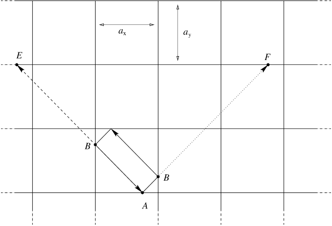
FIG. 11.: The stationary phase contributions for periodic orbits

The variable $s_{1}$ is such that it corresponds to the point $A$ in Fig. 11. The integral over the rest of the variables will give contributions corresponding to the orbit of interest when $s_{2}$ corresponds to either of the two points marked by $B$. These contributions are contributions of the orbit and its time reversal, and when either $N=0$ or $M=0$ there will be only one contributing point. From the composition law the result of the integral over $s_{2},\cdots,s_{n}$ (in the semiclassical limit) is the sum of the Green’s functions from the image points $E$ and $F$ to $A$. These contributions (and also their normal derivatives) are equal. For every point on the lower side there is a stationary phase contribution corresponding to an orbit (unless $N=0)$. This demonstrates that the periodic orbits are arranged in families. The contribution to the $s_{1}$ integral (in (A12)) from the lower side is thus

$$-4\int_{l.s.}ds_{1}\;\partial_{n_{1}}\frac{(-1)^{2N+2M-1}}{\sqrt{8\pi kl_{p}}}e^{i(kl_{p}-\frac{3}{4}\pi)}\simeq 4\frac{2Ma_{x}a_{y}i}{\sqrt{8\pi kl_{p}}}\frac{k}{l_{p}}e^{i(kl_{p}-\frac{3}{4}\pi)}$$ (A14)

where $l_{p}=\sqrt{(2Na_{x})^{2}+(2Ma_{y})^{2}}$ is the length of the periodic orbit, and $(N,M)$ is denoted by $p$. The factor of $-4$ is present since there was a factor of $-2$ in front of the integral (A12) that was not used in the composition law and also there are two equal contributions from the orbit and its time reversed one. In the semiclassical limit the dominant contribution of the partial derivative in (A12) is when it is applied to the exponent since it contributes a factor of $k$. The fact that $\partial_{n_{1}}l_{p}=\frac{2Ma_{y}}{l_{p}}$ was also used. The integrand is constant and thus the integral is just a multiplication by the side length $a_{x}$.

The contribution from the top side is equal to the one from the bottom side, and on the vertical side a similar calculation can be done, and one obtains the same contribution with the roles of $N$ and $M$ interchanged. The leading contribution (in the semiclassical limit) is obtained when the derivative $\frac{d}{dk}$ is applied to the exponential in (A12). The resulting contribution of the periodic orbit $p$ is thus

$$d_{osc}^{(N,M)}(k)=\frac{1}{\pi}\Im\frac{1}{2M+2N}\frac{d}{dk}\left(\frac{8{\cal A}\beta_{(N,M)}}{\sqrt{8\pi kl_{p}}}\frac{k}{l_{p}}(2M+2N)e^{i(kl_{p}-\frac{1}{4}\pi)}\right)\simeq\frac{8{\cal A}k\beta_{(N,M)}}{\pi\sqrt{8\pi kl_{p}}}\cos(kl_{p}-\frac{\pi}{4}),$$ (A15)

where $\beta(N,M)$ is a counting factor taking the values $1$ and $\frac{1}{2}$. Since the orbits with a vanishing index are their own time reversals, there is only one contribution for the $s_{2},\cdots,s_{n}$ integrals, therefore $\beta_{(N,M)}$ is equal to $\frac{1}{2}$ when $N=0$ or $M=0$ and is otherwise $1$.

The density of states measured in units of energy is $d(E)=\frac{d(k)}{2k}$. The contribution of a periodic orbits is thus given by

$$d_{osc}^{(N,M)}(E)=\frac{4{\cal A}\beta_{(N,M)}}{\pi\sqrt{8\pi kl_{p}}}\cos(kl_{p}-\frac{\pi}{4}).$$ (A16)

This is exactly the contribution that can be obtained using the Berry-Tabor formula for integrable systems [26].

2 Diffracting orbits

The contribution of diffracting orbits, with one diffraction, to the integrals (A3) results from terms where for one Green’s function the contribution of the second terms in (A4) is used while for the other $n-1$ terms the first term in (A4) is used. There are $n$ such terms, which are all equal (they only differ by the labels of the integration variables). To compute the contribution of diffracting orbits one has to evaluate the integral

$$I_{1}=(-2)^{n}\!\oint\!ds_{1}ds_{2}\cdots ds_{n}\,\partial_{n_{1}}\!G_{0}(k;{\bf r}_{2},{\bf r}_{1})\cdots\partial_{n_{n-1}}\!G_{0}(k;{\bf r}_{n},{\bf r}_{n-1})\partial_{n_{n}}\!G_{0}(k;{\bf r}_{0},{\bf r}_{n})D(\theta_{1},\theta_{n})G_{0}(k;{\bf r}_{1},{\bf r}_{0}).$$ (A17)

It will be assumed that the diffraction constant $D$ is slowly varying so that in the region which gives the stationary phase contribution it can be approximated by a constant. This means that $D(\theta,\theta^{\prime})$ does not change considerably when the angles change by $\delta\theta\sim\sqrt{\frac{\lambda}{l_{\bot}}}$ where $l_{\bot}$ is the distance from the scatterer to the hard wall. When $D$ is indeed slowly varying it can be replaced by its value at the stationary points of the boundary integrals and the composition law can be used to replace the integral (A17) by the sum of all Green’s functions from images of the scatterer (which cross $n$ walls) to the scatterer.

One can denote the once-diffracting orbits by the number of times they are reflected from the vertical and horizontal sides of the rectangle. For a pair of indices $(N_{1},M_{1})$ there are four (two when one of the indices vanishes) such orbits as can be seen from Fig. 12.

FIG. 12.: The $(1,2)$ once diffracting orbits

The dots in the figure denote the scatterer and its images, the orbits shown are all $(1,2)$ diffracting orbits. The contributions of these orbits will result from the integral with $3$ boundary points (there are also other contributions with $N_{1}+M_{1}=3$). Typically, there are four such orbits, but when one of the indices vanishes there are only two. We will add another index $\mu$ which runs between $1$ and $4$ and counts these orbits (alternatively it is possible to allow the indices $M_{1},N_{1}$ to be negative). The direction in which the diffracting orbit returns to the scatterer depends upon the outgoing direction and upon the parity of $(N_{1},M_{1})$. By counting the number of reflections on the boundary one finds

$$\theta_{in}=\Theta_{(N_{1},M_{1})}(\theta_{out})=\left\{{\begin{array}[]{ll}\theta_{out}&even-even\\ \pi-\theta_{out}&odd-even\\ 2\pi-\theta_{out}&even-odd\\ \pi+\theta_{out}&odd-odd.\end{array}}\right.$$ (A18)

In the example of Fig. 12 the parity of $(N_{1},M_{1})$ is odd-even. The lengths of the orbits and the angles can be calculated easily. If the scatterer is at $(a_{x}\delta_{x},a_{y}\delta_{y})$ from the center of the rectangle then the lengths of odd-odd orbits are given by $l_{p}^{(o-o)}=\sqrt{a_{x}^{2}(N_{1}\pm 2\delta_{x})^{2}+a_{y}^{2}(M_{1}\pm 2\delta_{y})^{2}}$. The angles can be computed similarly, since $\tan(\theta)=\frac{\pm N_{1}a_{x}+2a_{x}\delta_{x}}{\pm M_{1}a_{y}+2a_{y}\delta_{y}}$ (note that this angle is in the third quadrant if both the numerator and denominator are negative). The lengths and angles of other orbits can be computed too, just by replacing $\delta_{x}$ by $0$ when $N_{1}$ is even and $\delta_{y}$ by $0$ for even $M_{1}$.

The contribution to the integral (A17) which corresponds to the $(N_{1},M_{1})$ once diffracting orbits is thus

$$I_{1}^{(N_{1},M_{1})}=\sum_{\mu}(-1)^{N_{1}+M_{1}}D(\theta_{{\bf N}_{1},\mu},\Theta(\theta_{{\bf N}_{1},\mu}))\frac{1}{\sqrt{8\pi kl_{{\bf N}_{1},\mu}}}e^{i(kl_{{\bf N}_{1},\mu}-\frac{3}{4}\pi)}$$ (A19)

where $\mu$ runs over the four contributions (two contribution when either $M_{1}$ or $N_{1}$ vanish) and ${\bf N}_{1}=(N_{1},M_{1})$ is the pair of indices that define the orbits. In what follows some of the subscripts ${\bf N}_{j}$ will be replaced by $j$, that is $l_{{\bf N}_{j}}=l_{j}$, $\theta_{{\bf N}_{j}}=\theta_{j}$, etc. The contribution of each one of these orbits to the density of states is

$$\tilde{d}_{osc}^{(N_{1},M_{1}),\mu}(k)=\frac{1}{\pi}\Im\frac{d}{dk}\left((-1)^{N_{1}+M_{1}}D(\theta_{1,\mu},\Theta(\theta_{1,\mu}))\frac{1}{\sqrt{8\pi kl_{1,\mu}}}e^{i(kl_{1,\mu}-\frac{3}{4}\pi)}\right)$$ (A20)

In the semiclassical limit the main contribution is from the differentiation of the exponent. Thus the contribution of a once diffracting orbit is given by

$$\tilde{d}_{osc}^{(N_{1},M_{1}),\mu}(k)=(-1)^{N_{1}+M_{1}}\frac{\sqrt{l_{1,\mu}}}{\pi\sqrt{8\pi k}}\Re\left(D(\theta_{1,\mu},\Theta(\theta_{1,\mu}))e^{i(kl_{1,\mu}-\frac{3}{4}\pi)}\right).$$ (A21)

The contribution to $d(E)$ is thus

$$\tilde{d}_{osc}^{(N_{1},M_{1}),\mu}(E)=(-1)^{N_{1}+M_{1}}\frac{\sqrt{l_{1,\mu}}}{2\pi k\sqrt{8\pi k}}\Re\left(D(\theta_{1,\mu},\Theta(\theta_{1,\mu}))e^{i(kl_{1,\mu}-\frac{3}{4}\pi)}\right).$$ (A22)

The contribution of orbits with two diffractions is also needed in this work. The computation is quite similar, since these orbits are just a combination of two once diffracting orbits they can be identified by two pairs of integer indices ${\bf N}_{1}=(N_{1},M_{1})$ and ${\bf N}_{2}=(M_{2},N_{2})$ and by two indices $\mu$ ($\nu$ respectively) which denote along with the ${\bf N}_{1}$ (${\bf N}_{2}$ respectively) orbits that are parts of the twice diffracting orbit. The number of boundary reflections of each segment of the orbit is denoted by ${\cal N}_{i}=N_{i}+M_{i}$. The contribution of such an orbit to the density of states results from terms with two diffraction coefficients in the integral (A3) with $n={\cal N}_{1}+{\cal N}_{2}$. Not all of these terms describe a desired orbit, since only terms in which the number of reflections between diffractions is ${\cal N}_{1}$ (and also ${\cal N}_{2}$ since the orbits is closed) can describe the specified orbit. There are $\frac{n}{2}$ such contributions if ${\cal N}_{1}={\cal N}_{2}$ and $n$ contributions otherwise. If ${\cal N}_{1}\neq{\cal N}_{2}$ there are $n$ equal contributions that can be represented by an integral in which the first diffraction is, for instance, between ${\bf r}_{1}$ and ${\bf r}_{2}$ and the second one is after ${\cal N}_{1}$ reflections from the boundary (the orbit is closed after additional ${\cal N}_{2}$ reflections from the boundary). One can interchange ${\cal N}_{1}$ and ${\cal N}_{2}$ without changing the resulting contribution. It is convenient to split this contribution into two equal integrals in which the roles of ${\cal N}_{1}$ and ${\cal N}_{2}$ are interchanged. Each of these integrals, with the diffractions between ${\bf r}_{1}$ and ${\bf r}_{2}$ and between ${\bf r}_{{\cal N}_{1}+1}$ and ${\bf r}_{{\cal N}_{1}+2}$, should be multiplied by $\frac{n}{2}$ to take into account all permutations. Therefore all of the contributions of orbits with two diffractions are given by

$$d_{osc}^{(2)}(k) = \frac{1}{\pi}\frac{d}{dk}\Im\sum_{n=1}^{\infty}\frac{1}{n}\frac{n}{2}\sum_{{\cal N}_{1},{\cal N}_{2}=1}^{\infty}\delta_{{\cal N}_{1}+{\cal N}_{2},n}(-2)^{{\cal N}_{1}+{\cal N}_{2}}\int_{\partial{\cal D}}ds_{1}\cdots ds_{{\cal N}_{1}+{\cal N}_{2}}\partial_{{n}_{{\cal N}_{1}+{\cal N}_{2}}}G_{0}({\bf r}_{1},{\bf r}_{{\cal N}_{1}+{\cal N}_{2}})$$ (A23)

$$\times \partial_{{n}_{{\cal N}_{1}+{\cal N}_{2}-1}}G_{0}({\bf r}_{{\cal N}_{1}+{\cal N}_{2}},{\bf r}_{{\cal N}_{1}+{\cal N}_{2}-1})\cdots\partial_{{n}_{{\cal N}_{1}+2}}G_{0}({\bf r}_{{\cal N}_{1}+3},{\bf r}_{{\cal N}_{1}+2})G_{0}({\bf r}_{{\cal N}_{1}+2},{\bf r}_{0})D$$ (A24)

$$\times \partial_{{n}_{{\cal N}_{1}+1}}G_{0}({\bf r}_{0},{\bf r}_{{\cal N}_{1}+1})\partial_{n_{{\cal N}_{1}}}G_{0}({\bf r}_{{\cal N}_{1}+1},{\bf r}_{{\cal N}_{1}})\cdots\partial_{n_{2}}G_{0}({\bf r}_{3},{\bf r}_{2})G_{0}({\bf r}_{2},{\bf r}_{0})D\partial_{n_{1}}G_{0}({\bf r}_{0},{\bf r}_{1}).$$ (A25)

The dependence of $D$ on angles and of $G_{0}$ on $k$ was omitted in the notations for the sake of brevity. The sum over $n$ is trivial. The terms of this sum (which are products of two integrals) can be calculated using the composition rule. The result is a sum over all possible classical paths from the scatterer to itself with ${\cal N}_{1}$ reflections for the first segment (and ${\cal N}_{2}$ for the second). The contribution that corresponds to all of the twice diffracting orbits is thus

$$d_{osc}^{(2)}(k)=\sum_{{\bf N}_{1}\mu,{\bf N}_{2}\nu}\frac{1}{\pi}\frac{d}{dk}\Im(-1)^{N_{1}+M_{1}+N_{2}+M_{2}}D(\theta_{1,\mu},\Theta(\theta_{2,\nu}))\times$$ (A26)

$$D(\theta_{2,\nu},\Theta(\theta_{1,\mu}))\frac{1}{16\pi k\sqrt{l_{1,\mu}l_{2,\nu}}}e^{i(k(l_{1,\mu}+l_{2,\nu})-\frac{3}{2}\pi)}$$ (A27)

The dependence of the diffraction constants on the angles results from the fact that the in-going direction before the second diffraction is determined by the out-going direction from the first diffraction and vice versa. The relation between the out-going and in-going direction is given by (A18). In the leading order the derivative in (A23) operates only on the exponential, leading to the (energy dependent) density

$$d_{osc}^{(2)}(E)=\sum_{{\bf N}_{1}\mu,{\bf N}_{2}\nu}(-1)^{N_{1}+M_{1}+N_{2}+M_{2}}\frac{l_{1,\mu}+l_{2,\nu}}{32\pi^{2}k^{2}\sqrt{l_{1,\mu}l_{2,\nu}}}\times$$ (A28)

$$\Re\left(D(\theta_{1,\mu},\Theta(\theta_{2,\nu}))D(\theta_{2,\nu},\Theta(\theta_{1,\mu}))e^{i(k(l_{1,\mu}+l_{2,\nu})-\frac{3}{2}\pi)}\right).$$ (A29)

Combining (A28) with (A16) and (A22) we find that the total density of states taking into account terms up to the second order in $D$ is given by

$$d_{osc}(E) = \sum_{{\bf N}}\frac{2ab\beta_{(N,M)}}{\pi\sqrt{8\pi kl_{p}}}e^{i(kl_{p}-\frac{\pi}{4})}+\sum_{{\bf N}_{1},\mu}(-1)^{N_{1}+M_{1}}\frac{\sqrt{l_{1,\mu}}}{4\pi k\sqrt{8\pi k}}D(\theta_{1,\mu},\Theta(\theta_{1,\mu}))e^{i(kl_{1,\mu}-\frac{3}{4}\pi)}$$ (A30)

$$+ \sum_{{\bf N}_{1},\mu}\sum_{{\bf N}_{2},\nu}(-1)^{N_{1}\!+\!M_{1}\!+\!N_{2}\!+\!M_{2}}\frac{l_{1,\mu}+l_{2,\nu}}{64\pi^{2}k^{2}\sqrt{l_{1,\mu}l_{2,\nu}}}\left(D(\theta_{1,\mu},\Theta(\theta_{2,\nu}))D(\theta_{2,\nu},\Theta(\theta_{1,\mu}))e^{i(k(l_{1,\mu}+l_{2,\nu})-\frac{3}{2}\pi)}\right)$$ (A31)

$$+ c.c.$$ (A32)

Note that when one of the indices of ${\bf N}_{1}$ (${\bf N}_{2}$ respectively) vanishes the sum over $\mu$ ($\nu$ respectively) includes two contributions instead of four. Thus for an angle independent diffraction constant such orbits will have a factor of half similar to the one that appears in the periodic orbit contributions. Equation (A30) will be used to compute the various contributions to the spectral from factor.

Similarly one can calculate the contributions of orbits with three diffraction. The calculation follows the one of two diffractions closely, and the only difference is that one now has a factor of $\frac{n}{3}$ instead of $\frac{n}{2}$ in (A23). Since there are three diffractions the sum is over ${\bf N}_{1},\mu_{1}$, ${\bf N}_{2},\mu_{2}$ and ${\bf N}_{3},\mu_{3}$ which describe the three segments of the orbits. In this work the contribution to third order in $D$ is required only for angle independent scattering. In this case the contribution of all orbits with three (angle independent) diffractions is found to be

$$d_{osc}^{(3)}(E) = \sum_{{\bf N}_{1},\mu_{1}}\sum_{{\bf N}_{2},\mu_{2}}\sum_{{\bf N}_{3},\mu_{3}}(-1)^{N_{1}+M_{1}+N_{2}+M_{2}+N_{3}+M_{3}}\frac{D^{3}}{12\pi k(8\pi k)^{\frac{3}{2}}}\frac{l_{1,\mu_{1}}+l_{2,\mu_{2}}+l_{3,\mu_{3}}}{\sqrt{l_{1,\mu_{1}}l_{2,\mu_{2}}l_{3,\mu_{3}}}}e^{-i\frac{\pi}{4}}$$ (A33)

$$\times e^{ik(l_{1,\mu_{1}}+l_{2,\mu_{2}}+l_{3,\mu_{3}})}+c.c.$$ (A34)

In Sec. II it is assumed that the scattering is angle independent, therefore the function $D(\theta,\theta^{\prime})$ is replaced by an angle independent constant $D$. Moreover we are interested in the form factor where in the calculation energy averages are taken and sums over periodic orbits are approximated by integrals. Within such approximations the weight of the orbits with $\beta_{(N,M)}\neq 1$ (one vanishing index) is negligible, therefore in other parts of the paper these factors were replaced by unity. Within these assumptions (A30) and (A33) reduce to (8).

B The diffraction constant of the point scatterer with the free Green’s function $G_{0}$

The diffraction constant is the on shell transition matrix, $T$, which for a point interaction is given by

$$D^{-1}(z)=\frac{z-i\Lambda}{1-e^{i\xi_{1}}}\int d^{2}{x}\;G_{0}(z;{\bf x},{\bf 0})G_{0}(i\Lambda;{\bf x},{\bf 0})+\frac{z+i\Lambda}{1-e^{-i\xi_{1}}}\int d^{2}{\bf x}\;G_{0}(z;{\bf x},{\bf 0})G_{0}(-i\Lambda;{\bf x},{\bf 0})$$ (B1)

where $\Im\sqrt{z}>0$ and $G_{0}$ is the Green’s function in free space. To compute the integrals we use the following integral representation for the free Green’s function in two dimensions

$$G_{0}(z;{\bf x},{\bf x}_{0})=\frac{1}{(2\pi)^{2}}\int d^{2}k\;\frac{e^{i{\bf k}\cdot({\bf x}_{0}-{\bf x})}}{z-k^{2}}.$$ (B2)

Let us compute the integral

$$I_{1} = \int d^{2}{x}\;G_{0}(z;{\bf x},{\bf 0})G_{0}(i\Lambda;{\bf x},{\bf 0})=\frac{1}{(2\pi)^{4}}\int d^{2}k_{1}\;d^{2}k_{2}\;d^{2}x\;\frac{e^{-i{\bf k}_{1}\cdot{\bf x}}}{(k_{1}^{2}-z)}\frac{e^{-i{\bf k}_{2}\cdot{\bf x}}}{(k_{2}^{2}-i\Lambda)}$$ (B3)

$$= \frac{1}{(2\pi)^{2}}\int d^{2}k\;\frac{1}{(k^{2}-z)(k^{2}-i\Lambda)}.$$ (B4)

Changing variables to $E=k^{2}$ one obtains

$$I_{1}=\frac{1}{4\pi}\int_{0}^{\infty}dE\;\frac{1}{(E-z)(E-i\Lambda)}=\frac{1}{4\pi(z-i\Lambda)}\int_{0}^{\infty}dE\;\left[\frac{1}{E-z}-\frac{1}{E-i\Lambda}\right].$$ (B5)

Using the known relation

$$\frac{1}{x-x_{0}\pm i\epsilon}=\wp{\frac{1}{x-x_{0}}}\mp i\pi\delta(x-x_{0})$$ (B6)

and noting that we are interested in the case where $\Im z$ tends to zero from above we obtain

$$I_{1}=\frac{1}{4\pi(z-i\Lambda)}\lim_{M\rightarrow\infty}\lim_{\beta\rightarrow 0}\left[\int_{0}^{z-\beta}dE\;\frac{1}{E-z}+\int_{z+\beta}^{M}dE\;\frac{1}{E-z}-\int_{0}^{M}dE\;\frac{1}{E-i\Lambda}+i\pi\right].$$ (B7)

The integrals are elementary, and taking the limits results in

$$I_{1}=\frac{1}{4\pi(z-i\Lambda)}\left[-\ln\left(\frac{z}{\Lambda}\right)+i\frac{\pi}{2}\right].$$ (B8)

The second integral in (B1) is computed in the same way

$$I_{2}=\int d^{2}x\;G_{0}(z;{\bf x},{\bf 0})G_{0}(-i\Lambda;{\bf x},{\bf 0})=\frac{1}{4\pi(z+i\Lambda)}\left[-\ln\left(\frac{z}{\Lambda}\right)+i\frac{3\pi}{2}\right].$$ (B9)

Substituting (B8) and (B9) into (B1) leads to the diffraction constant:

$$D(z)=\frac{2\pi}{-\frac{1}{2}\ln\left(\frac{z}{\Lambda}\right)+\frac{\pi}{4}\frac{\sin\xi_{1}}{1-\cos\xi_{1}}+i\frac{\pi}{2}}.$$ (B10)

C Asymptotics of scattering from localized potentials

In this Appendix $D_{g}({\bf q})$ and $h({\bf k},{\bf q})$ are computed up to order $k^{2}a^{2}$. The computation is presented explicitly only to order $ka$. The calculation of the second order is straight forward and fairly similar to the calculation of the first order, but its details are too long to be included in the paper.

1 Calculation of $D_{g}({\bf q})$ to the order $(qa)^{2}$

In the calculation of $D_{g}({\bf q})$ many of the contributions cancel, but equation (105) does not show this explicitly. A more convenient way to compute $D_{g}({\bf q})$ is obtained when (98) is iterated, and all the resolutions of the identity in momentum space which appear there are replaced by resolutions of identity in coordinate space. Using (95) leads to

$$D_{g} = 1-g\int d^{2}y_{1}^{(a)}d^{2}y_{1}\;e^{-ia{\bf q\cdot y}_{1}^{(a)}}f({\bf y}_{1}^{(a)})G_{0}(ka;{\bf y}_{1}^{(a)},{\bf y}_{1})\frac{f({\bf y}_{1})}{V_{0}}e^{ia{\bf q\cdot y}_{1}}$$ (C1)

$$- g^{2}\int d^{2}y_{1}^{(a)}d^{2}y_{1}d^{2}y_{2}\;e^{-ia{\bf q\cdot y}_{1}^{(a)}}f({\bf y}_{1}^{(a)})G_{0}(ka;{\bf y}_{1}^{(a)},{\bf y}_{1})\times$$ (C2)

$$\times \left(f({\bf y}_{1})G_{0}(ka;{\bf y}_{1},{\bf y}_{2})-\int d^{2}y_{2}^{(a)}\frac{f({\bf y}_{1})f({\bf y}_{2}^{(a)})}{V_{0}}e^{ia{\bf q\cdot}({\bf y}_{1}-{\bf y}_{2}^{(a)})}G_{0}(ka;{\bf y}_{2}^{(a)},{\bf y}_{2})\right)\frac{f({\bf y}_{2})}{V_{0}}e^{ia{\bf q\cdot y}_{2}}$$ (C3)

$$- g^{3}\int d^{2}y_{1}^{(a)}d^{2}y_{1}d^{2}y_{2}d^{2}y_{3}\;e^{-ia{\bf q\cdot y}_{1}^{(a)}}f({\bf y}_{1}^{(a)})G_{0}(ka;{\bf y}_{1}^{(a)},{\bf y}_{1})\times$$ (C4)

$$\times \!\left(f({\bf y}_{1})G_{0}(ka;{\bf y}_{1},{\bf y}_{2})-\!\int d^{2}y_{2}^{(a)}\frac{f({\bf y}_{1})f({\bf y}_{2}^{(a)})}{V_{0}}e^{ia{\bf q\cdot}({\bf y}_{1}-{\bf y}_{2}^{(a)})}G_{0}(ka;{\bf y}_{2}^{(a)},{\bf y}_{2})\right)\times$$ (C5)

$$\times \!\left(f({\bf y}_{2})G_{0}(ka;{\bf y}_{2},{\bf y}_{3})-\!\int\!d^{2}y_{3}^{(a)}\frac{f({\bf y}_{2})f({\bf y}_{3}^{(a)})}{V_{0}}e^{ia{\bf q\cdot}({\bf y}_{2}-{\bf y}_{3}^{(a)})}G_{0}(ka;{\bf y}_{3}^{(a)},{\bf y}_{3})\right)\!\frac{f({\bf y}_{3})}{V_{0}}e^{ia{\bf q\cdot y}_{3}}-\cdots$$ (C6)

where

$$V_{0}=\langle{\bf q}|{\bf U}|{\bf q}\rangle=\int d^{2}yf({\bf y}).$$ (C7)

The terms of higher order in $g$ have the same structure, but with more of the factors such as

$$B_{j}=f({\bf y}_{j})G_{0}(ka;{\bf y}_{j},{\bf y}_{j+1})-\int d^{2}y_{j+1}^{(a)}\frac{f({\bf y}_{j})f({\bf y}_{j+1}^{(a)})}{V_{0}}e^{ia{\bf q\cdot}({\bf y}_{j}-{\bf y}_{j+1}^{(a)})}G_{0}(ka;{\bf y}_{j+1}^{(a)},{\bf y}_{j+1}).$$ (C8)

Equation (C1) is a convenient starting point from which the asymptotics of $D_{g}({\bf q})$ in the limit $qa\rightarrow 0$ can be calculated .

To calculate the leading order of $D_{g}({\bf q})$ (with respect to $qa$) all the exponentials are replaced by unity and the Green’s function by the leading order as given by (108). The leading order of any of the brackets is given by

$$B_{j}\simeq f({\bf y}_{j})\phi({\bf y}_{j},{\bf y}_{j+1})-\int d^{2}y_{j+1}^{(a)}\frac{f({\bf y}_{j})f({\bf y}_{j+1}^{(a)})}{V_{0}}\phi({\bf y}_{j+1}^{(a)},{\bf y}_{j+1}).$$ (C9)

Note that the contribution from the constant parts of the Green’s functions, $d_{1}$, cancel each other. This is the advantage of the Noyce method when describing scattering at low energies in two dimensions. Most of the Green’s functions in equation (C1) appear in brackets of the form $B_{j}$, and thus, in the leading order, their constant parts cancel. However, in every term of some power in $g$ there is one Green’s function that does not appear in some brackets. When this Green’s function is multiplied by one of the brackets one finds that the contribution of its constant part, $d_{1}$, vanishes. This is true since for any functions $g_{1}({\bf y})$,$g_{2}({\bf y})$, $G({\bf y}_{1},{\bf y}_{2})$ one finds

$$\int d^{2}y_{1}^{(a)}d^{2}y_{1}d^{2}y_{2}\;g_{1}({\bf y}_{1}^{(a)})d_{1}\left(f({\bf y}_{1})G({\bf y}_{1},{\bf y}_{2})-\int d^{2}y_{2}^{(a)}\frac{f({\bf y}_{1})f({\bf y}_{2}^{(a)})}{V_{0}}G({\bf y}_{2}^{(a)},{\bf y}_{2})\right)g_{2}({\bf y}_{2}) =$$ (C10)

$$\int d^{2}y_{1}^{(a)}d^{2}y_{2}\;g_{1}({\bf y}_{1}^{(a)})d_{1}\left(\int d^{2}y_{1}f({\bf y}_{1})G({\bf y}_{1},{\bf y}_{2})-\int d^{2}y_{2}^{(a)}f({\bf y}_{2}^{(a)})G({\bf y}_{2}^{(a)},{\bf y}_{2})\right)g_{2}({\bf y}_{2}) = 0.$$ (C11)

Therefore the constant part of the Green’s function does not contribute to the leading order of $D_{g}({\bf q})$ except for the term of order $g$. Using (C9) and (C10) the leading order (in $qa$) contribution to $D_{g}({\bf q})$ is given by

$$D_{g} \simeq 1-g\int d^{2}y_{1}^{(a)}d^{2}y_{1}\;f({\bf y}_{1}^{(a)})\left(d_{1}+\phi({\bf y}_{1}^{(a)},{\bf y}_{1})\right)\frac{f({\bf y}_{1})}{V_{0}}$$ (C12)

$$- \!g^{2}\int\!d^{2}y_{1}^{(a)}d^{2}y_{1}d^{2}y_{2}\;f({\bf y}_{1}^{(a)})\phi({\bf y}_{1}^{(a)},{\bf y}_{1})\left(f({\bf y}_{1})\phi({\bf y}_{1},{\bf y}_{2})-\int\!d^{2}y_{2}^{(a)}\frac{f({\bf y}_{1})f({\bf y}_{2}^{(a)})}{V_{0}}\phi({\bf y}_{2}^{(a)},{\bf y}_{2})\right)\frac{f({\bf y}_{2})}{V_{0}}$$ (C13)

$$- \!g^{3}\int\!d^{2}y_{1}^{(a)}d^{2}y_{1}d^{2}y_{2}d^{2}y_{3}\;f({\bf y}_{1}^{(a)})\phi({\bf y}_{1}^{(a)},{\bf y}_{1})\left(f({\bf y}_{1})\phi({\bf y}_{1},{\bf y}_{2})-\int\!d^{2}y_{2}^{(a)}\frac{f({\bf y}_{1})f({\bf y}_{2}^{(a)})}{V_{0}}\phi({\bf y}_{2}^{(a)},{\bf y}_{2})\right)$$ (C14)

$$\times \left(f({\bf y}_{2})\phi({\bf y}_{2},{\bf y}_{3})-\int\!d^{2}y_{3}^{(a)}\frac{f({\bf y}_{2})f({\bf y}_{3}^{(a)})}{V_{0}}\phi({\bf y}_{3}^{(a)},{\bf y}_{3})\right)\frac{f({\bf y}_{3})}{V_{0}}-\cdots.$$ (C15)

Note that the integrals in (C12) are angle independent. To simplify the notations the following definitions are useful

$$L_{0} \equiv \int d^{2}y_{1}\;f({\bf y}_{1})=V_{0}$$ (C16)

$$L_{1} \equiv \int d^{2}y_{1}d^{2}y_{2}\;f({\bf y}_{1})\phi({\bf y}_{1},{\bf y}_{2})f({\bf y}_{2})$$ (C17)

$$L_{2} \equiv \int d^{2}y_{1}d^{2}y_{2}d^{2}y_{3}\;f({\bf y}_{1})\phi({\bf y}_{1},{\bf y}_{2})f({\bf y}_{2})\phi({\bf y}_{2},{\bf y}_{3})f({\bf y}_{3})$$ (C18)

$$\vdots$$ (C19)

Using these definitions (C12) can be written as

$$D_{g}({\bf q})\simeq 1-gd_{1}V_{0}-g\frac{L_{1}}{V_{0}}-g^{2}\left(\frac{L_{2}}{V_{0}}-\frac{L_{1}^{2}}{V_{0}^{2}}\right)-g^{3}\left(\frac{L_{3}}{V_{0}}-2\frac{L_{2}L_{1}}{V_{0}^{2}}+\frac{L_{1}^{3}}{V_{0}^{3}}\right)-\cdots$$ (C20)

Note that the contribution of order $g^{N}$ is a sum where each term is composed of a product of $L_{j}$’s where the sum of $j$’s is $N$. It is multiplied by $-\frac{1}{V_{0}}$ to the power of number of $L_{j}$’s. The sum is over all possible partitions of $N$ into positive integer numbers $m_{j}$ so that $\sum_{j}m_{j}=N$. Such partitions are generated by the expansion

$$V(g)=\frac{V_{0}}{\sum_{m=0}^{\infty}g^{m}L_{m}}=\frac{V_{0}}{V_{0}+\sum_{m=1}^{\infty}g^{m}L_{m}}=1+\sum_{k=1}^{\infty}\left[-\sum_{m=1}^{\infty}g^{m}\frac{L_{m}}{V_{0}}\right]^{k},$$ (C21)

that can be written in terms of partitions as

$$V(g)=1+\sum_{N=1}^{\infty}g^{N}\sum_{i}\prod_{j=1}^{l_{i}}\left(-\frac{L_{m_{j}}}{V_{0}}\right),$$ (C22)

where $i$ is the index that specifies the $i$-th partition consisting of $l_{i}$ terms. The various indices of the $i$-th partition satisfy $\sum_{j=1}^{l_{i}}m_{j}=N$ with the requirement that all $m_{j}$ are positive. Consequently the leading order of $D_{g}({\bf q})$ is

$$D_{g}({\bf q})=V(g)-gd_{1}V_{0}.$$ (C23)

Expanding $V(g)$ to the order $g^{3}$ one recovers (C20).

There are no contributions to $D_{g}({\bf q})$ of order $qa$ and the first correction to $D_{g}({\bf q})$ scales as $q^{2}a^{2}$ (times some power of $\ln qa$). To see this note that from (105) it is clear that $D_{g}({\bf q})$ is built from products of matrix elements of the form $\langle{\bf q}|{\bf UGUGU\cdots UGU}|{\bf q}\rangle$ with various numbers of Green’s functions. A contribution of the order $qa$ must come from one of these elements which is expanded to that order. For example, the contribution of $\langle{\bf q}|{\bf UGU}|{\bf q}\rangle$ to this order is

$$-\int d^{2}y_{1}d^{2}y_{2}\;ia{\bf q\cdot y}_{1}f({\bf y}_{1})G_{0}(ka;{\bf y}_{1},{\bf y}_{2})f({\bf y}_{2})+\int d^{2}y_{1}d^{2}y_{2}\;ia{\bf q\cdot y}_{2}f({\bf y}_{1})G_{0}(ka;{\bf y}_{1},{\bf y}_{2})f({\bf y}_{2})=0,$$ (C24)

since $G_{0}(ka;{\bf y}_{1},{\bf y}_{2})=G_{0}(ka;{\bf y}_{2},{\bf y}_{1})$. This holds if more Green’s functions are used, therefore $D_{g}({\bf q})$ cannot have contributions of the order $qa$.

The contribution of higher order in $qa$ to $D_{g}({\bf q})$ can be computed by expanding the exponents and the Green’s functions in (C1) and collecting all the terms up to the required order of $qa$. Here $D_{g}({\bf q})$ is calculated to order $q^{2}a^{2}$. The calculation is straightforward but tedious and only the final result is presented

$$D_{g} \simeq V(g)-gd_{1}V_{0}+\frac{q^{2}a^{2}}{2}g\left(d_{1}-\frac{1}{2\pi}\right)V_{0}V(g)\left[\sum_{k=0}^{\infty}\frac{\delta_{k}}{V_{0}}g^{k}-V(g)\left|\sum_{k=0}^{\infty}\frac{\alpha_{k}}{V_{0}}g^{k}\right|^{2}\right]+\frac{q^{2}a^{2}}{4}V^{2}(g)\sum_{l=1}^{\infty}\frac{{{\cal L}_{l}}}{V_{0}}g^{l}$$ (C26)

$$-q^{2}a^{2}\left(V(g)-gd_{1}V_{0}\right)\left\{\left(V(g)-gd_{1}V_{0}\right)\sum_{l=1}^{\infty}\frac{e^{2i\theta}\mu_{l}^{(++)}+\mu_{l}^{(+-)}+\mu_{l}^{(-+)}+e^{-2i\theta}\mu_{l}^{(--)}}{4V_{0}}g^{l}\right.$$

$$- \left.\frac{gd_{1}}{2}\left(\delta_{0}+\frac{1}{2}e^{2i\theta}\sigma_{0}+\frac{1}{2}e^{-2i\theta}\sigma_{0}^{*}\right)-V(g)\sum_{l=1}^{\infty}\frac{\left(\delta_{l}+\frac{1}{2}e^{2i\theta}\sigma_{l}+\frac{1}{2}e^{-2i\theta}\sigma_{l}^{*}\right)}{2V_{0}}g^{l}\right.$$ (C27)

$$+ \left.V(g)gd_{1}V_{0}\left(\sum_{k=0}^{\infty}\frac{e^{i\theta}\alpha_{k}+e^{-i\theta}\alpha_{k}^{*}}{2V_{0}}g^{k}\right)^{2}\right\},$$ (C28)

where $\theta$ is the direction of the vector ${\bf q}$ in the plane. The constants ${\cal L}_{k}$, $\alpha_{k}$, $\delta_{k}$, $\sigma_{k}$ and $\mu_{k}^{(ab)}$ are independent of $\theta$ and $q$ and are defined in what follows. First we define

$${{\cal L}_{k}}\equiv\int d^{2}y_{1}\cdots d^{2}y_{k+1}\;\left(\sum_{j=1}^{k}({\bf y}_{j}-{\bf y}_{j+1})^{2}\right)f({\bf y}_{1})\phi({\bf y}_{1},{\bf y}_{2})f({\bf y}_{2})\times\cdots\times\phi({\bf y}_{k},{\bf y}_{k+1})f({\bf y}_{k+1})$$ (C29)

and

$$\alpha_{0} \equiv \int d^{2}y_{1}\;e^{-i\theta_{1}}|{\bf y}_{1}|f({\bf y}_{1})$$ (C30)

$$\alpha_{1} \equiv \int d^{2}y_{1}d^{2}y_{2}\;e^{-i\theta_{1}}|{\bf y}_{1}|f({\bf y}_{1})\phi({\bf y}_{1},{\bf y}_{2})f({\bf y}_{2})$$ (C31)

$$\alpha_{2} \equiv \int d^{2}y_{1}d^{2}y_{2}d^{2}y_{3}\;e^{-i\theta_{1}}|{\bf y}_{1}|f({\bf y}_{1})\phi({\bf y}_{1},{\bf y}_{2})f({\bf y}_{2})\phi({\bf y}_{2},{\bf y}_{3})f({\bf y}_{3})$$ (C32)

$$\vdots$$ (C33)

where $\theta_{1}$ denotes the direction of ${\bf y_{1}}$. The other constants are

$$\delta_{0} \equiv \int d^{2}y_{1}\;|{\bf y}_{1}|^{2}f({\bf y}_{1})$$ (C34)

$$\delta_{1} \equiv \int d^{2}y_{1}d^{2}y_{2}\;|{\bf y}_{1}|^{2}f({\bf y}_{1})\phi({\bf y}_{1},{\bf y}_{2})f({\bf y}_{2})$$ (C35)

$$\delta_{2} \equiv \int d^{2}y_{1}d^{2}y_{2}d^{2}y_{3}\;|{\bf y}_{1}|^{2}f({\bf y}_{1})\phi({\bf y}_{1},{\bf y}_{2})f({\bf y}_{2})\phi({\bf y}_{2},{\bf y}_{3})f({\bf y}_{3})$$ (C36)

$$\vdots$$ (C37)

$$\sigma_{0} \equiv \int d^{2}y_{1}\;e^{-2i\theta_{1}}|{\bf y}_{1}|^{2}f({\bf y}_{1})$$ (C38)

$$\sigma_{1} \equiv \int d^{2}y_{1}d^{2}y_{2}\;e^{-2i\theta_{1}}|{\bf y}_{1}|^{2}f({\bf y}_{1})\phi({\bf y}_{1},{\bf y}_{2})f({\bf y}_{2})$$ (C39)

$$\sigma_{2} \equiv \int d^{2}y_{1}d^{2}y_{2}d^{2}y_{3}\;e^{-2i\theta_{1}}|{\bf y}_{1}|^{2}f({\bf y}_{1})\phi({\bf y}_{1},{\bf y}_{2})f({\bf y}_{2})\phi({\bf y}_{2},{\bf y}_{3})f({\bf y}_{3})$$ (C40)

$$\vdots$$ (C41)

and

$$\mu_{0}^{(++)} \equiv \int d^{2}y_{1}\;e^{-i\theta_{1}}|{\bf y}_{1}|f({\bf y}_{1})|{\bf y}_{1}|e^{-i\theta_{1}}$$ (C42)

$$\mu_{1}^{(++)} \equiv \int d^{2}y_{1}d^{2}y_{2}\;e^{-i\theta_{1}}|{\bf y}_{1}|f({\bf y}_{1})\phi({\bf y}_{1},{\bf y}_{2})f({\bf y}_{2})|{\bf y}_{2}|e^{-i\theta_{2}}$$ (C43)

$$\mu_{1}^{(+-)} \equiv \int d^{2}y_{1}d^{2}y_{2}\;e^{-i\theta_{1}}|{\bf y}_{1}|f({\bf y}_{1})\phi({\bf y}_{1},{\bf y}_{2})f({\bf y}_{2})|{\bf y}_{2}|e^{+i\theta_{2}}$$ (C44)

$$\mu_{2}^{(++)} \equiv \int d^{2}y_{1}d^{2}y_{2}d^{2}y_{3}\;e^{-i\theta_{1}}|{\bf y}_{1}|f({\bf y}_{1})\phi({\bf y}_{1},{\bf y}_{2})f({\bf y}_{2})\phi({\bf y}_{2},{\bf y}_{3})f({\bf y}_{3})|{\bf y}_{3}|e^{-i\theta_{3}}$$ (C45)

$$\mu_{2}^{(--)} \equiv \int d^{2}y_{1}d^{2}y_{2}d^{2}y_{3}\;e^{i\theta_{1}}|{\bf y}_{1}|f({\bf y}_{1})\phi({\bf y}_{1},{\bf y}_{2})f({\bf y}_{2})\phi({\bf y}_{2},{\bf y}_{3})f({\bf y}_{3})|{\bf y}_{3}|e^{i\theta_{3}}$$ (C46)

$$\vdots$$ (C47)

where the lower index specifies the number of $\phi$’s in the integrals and the upper index is the opposite of the sign of the angles in the exponents. Note that

$$\mu_{k}^{(-+)}={\mu_{k}^{(+-)}}^{*}\;\;\;,\;\;\;\mu_{k}^{(--)}={\mu_{k}^{(++)}}^{*}$$ (C48)

In addition to these definitions, for future use, it is also convenient to define the sums

$$\alpha(g)\equiv\sum_{k=0}^{\infty}\alpha_{k}g^{k}$$ (C49)

$$\delta(g)\equiv\sum_{k=0}^{\infty}\delta_{k}g^{k}$$ (C50)

$$\sigma(g)\equiv\sum_{k=0}^{\infty}\sigma_{k}g^{k}$$ (C51)

$$\mu^{(ab)}(g)\equiv\sum_{k=0}^{\infty}\mu_{k}^{(ab)}g^{k}.$$ (C52)

2 Expansion of $h({\bf k},{\bf q})$ for $ka$ and $qa\ll 1$

The most convenient way to obtain the expansion of $h({\bf k},{\bf q})$ for small $ka$ and $qa$ is by iterating (98) and inserting resolutions of the identity (in coordinate representation) where appropriate. Note that by definition (94), $h({\bf q},{\bf q})=1$. Changing the integration variables to ${\bf y}_{i}=\frac{{\bf r}_{i}}{a}$ results in:

$$h({\bf k},{\bf q}) = \int d^{2}y_{0}e^{-ia({\bf k-q})\cdot{\bf y}_{0}}\frac{f({\bf y}_{0})}{V_{0}}+g\int d^{2}y_{0}d^{2}y_{1}\left(\rule{0.0pt}{19.91692pt}e^{-ia{\bf k}\cdot{\bf y}_{0}}f({\bf y}_{0})G_{0}(ka;{\bf y}_{0},{\bf y}_{1})\right.$$ (C53)

$$- \left.\int d^{2}y_{1}^{(a)}\;\frac{f({\bf y}_{0})f({\bf y}_{1}^{(a)})}{V_{0}}e^{ia({\bf q-k})\cdot{\bf y}_{0}}e^{-ia{\bf q}\cdot{\bf y}_{1}^{(a)}}G_{0}(ka;{\bf y}_{1}^{(a)},{\bf y}_{1})\right)\frac{f({\bf y}_{1})}{V_{0}}e^{ia{\bf q}\cdot{\bf y}_{1}}$$ (C54)

$$+ g^{2}\int d^{2}y_{0}d^{2}y_{1}d^{2}y_{2}\left(e^{-ia{\bf k}\cdot{\bf y}_{0}}f({\bf y}_{0})G_{0}(ka;{\bf y}_{0},{\bf y}_{1})-\int d^{2}y_{1}^{(a)}\frac{f({\bf y}_{0})f({\bf y}_{1}^{(a))}}{V_{0}}e^{ia({\bf q-k})\cdot{\bf y}_{0}}\right.$$ (C55)

$$\times \left.e^{-ia{\bf q}\cdot{\bf y}_{1}^{(a)}}G_{0}(ka;{\bf y}_{1}^{(a)},{\bf y}_{1})\rule{0.0pt}{19.91692pt}\right)$$ (C56)

$$\times \left(f({\bf y}_{1})G_{0}(ka;{\bf y}_{1},{\bf y}_{2})-\int d^{2}y_{2}^{(a)}\frac{f({\bf y}_{1})f({\bf y}_{2}^{(a)})}{V_{0}}e^{ia{\bf q}\cdot({\bf y}_{1}-{\bf y}_{2}^{(a)})}G_{0}(ka;{\bf y}_{2}^{(a)},{\bf y}_{2})\right)\frac{f({\bf y}_{2})}{V_{0}}e^{ia{\bf q}\cdot{\bf y}_{2}}$$ (C57)

$$+ \cdots$$ (C58)

The general term in this series is composed of a first factor

$$A_{0}({\bf y}_{0},{\bf y}_{1})=e^{-ia{\bf k}\cdot{\bf y}_{0}}f({\bf y}_{0})G_{0}(ka;{\bf y}_{0},{\bf y}_{1})-\int d^{2}y_{1}^{(a)}\frac{f({\bf y}_{0})f({\bf y}_{1}^{(a)})}{V_{0}}e^{ia({\bf q-k})\cdot{\bf y}_{0}}e^{-ia{\bf q}\cdot{\bf y}_{1}^{(a)}}G_{0}(ka;{\bf y}_{1}^{(a)},{\bf y}_{1})$$ (C59)

followed by several factors of the type $B_{j}$ defined by (C8), and a last factor

$$A_{N}=e^{ia{\bf q}\cdot{\bf y}_{N}}\frac{f({\bf y}_{N})}{V_{0}}$$ (C60)

(with all variables integrated). To compute the $ka$ and $qa$ dependence of $h({\bf k},{\bf q})$ every term in equation (C53) is expanded for small $ka$ ($qa$) and the whole series in $g$ is summed. In what follows $h({\bf k},{\bf q})$ will be computed to order $k^{2}a^{2}$ (and also $q^{2}a^{2}$, $kqa^{2}$).

To compute $h({\bf k},{\bf q})$ for small $ka$ the first factor has to be calculated at least to the first order $ka$. In this order

$$I({\bf y}_{1}) = \int d^{2}y_{0}A_{0}({\bf y}_{0},{\bf y}_{1})$$ (C61)

$$\simeq \int d^{2}y_{0}\;ia({\bf q-k})\cdot{\bf y}_{0}\left(f({\bf y}_{0})\phi({\bf y}_{0},{\bf y}_{1})-\int d^{2}y_{1}^{(a)}\frac{f({\bf y}_{0})f({\bf y}_{1}^{(a)})}{V_{0}}\phi({\bf y}_{1}^{(a)},{\bf y}_{1})\right).$$ (C62)

Note that in the leading (zeroth) order in $ka$ this contribution vanishes. This is related to the fact that by definition $h({\bf q},{\bf q})=1$, and in the leading order the direction of the momentum is not important. To compute $h({\bf k},{\bf q})$ up to order $ka$ the factors $B_{j}$ and $A_{N}$ can be taken in the leading order (zeroth order in $ka$). Using (C9) and (C61) one finds

$$h({\bf k},{\bf q}) = 1+ia\left\{\int d^{2}y_{0}\;({\bf q-k})\cdot{\bf y}_{0}\frac{f({\bf y}_{0})}{V_{0}}\right.$$ (C63)

$$+ g\int d^{2}y_{0}d^{2}y_{1}\;({\bf q-k})\cdot{\bf y}_{0}\left(f({\bf y}_{0})\phi({\bf y}_{0},{\bf y}_{1})-\int d^{2}y_{1}^{(a)}\frac{f({\bf y}_{0})f({\bf y}_{1}^{(a)})}{V_{0}}\phi({\bf y}_{1}^{(a)},{\bf y}_{1})\right)\frac{f({\bf y}_{1})}{V_{0}}$$ (C64)

$$+ g^{2}\int d^{2}y_{0}d^{2}y_{1}d^{2}y_{2}\;({\bf q-k})\cdot{\bf y}_{0}\left(f({\bf y}_{0})\phi({\bf y}_{0},{\bf y}_{1})-\int d^{2}y_{1}^{(a)}\frac{f({\bf y}_{0})f({\bf y}_{1}^{(a)})}{V_{0}}\phi({\bf y}_{1}^{(a)},{\bf y}_{1})\right)$$ (C65)

$$\times \left.\left(f({\bf y}_{1})\phi({\bf y}_{1},{\bf y}_{2})-\int d^{2}y_{2}^{(a)}\frac{f({\bf y}_{1})f({\bf y}_{2}^{(a)})}{V_{0}}\phi({\bf y}_{2}^{(a)},{\bf y}_{2})\right)\frac{f({\bf y}_{2})}{V_{0}}+\cdots\right\}$$ (C66)

Since ${\bf k}\cdot{\bf y}_{0}=k|{\bf y}_{0}|\cos(\theta^{\prime}-\theta_{0})$ (and ${\bf q}\cdot{\bf y}_{0}=q|{\bf y}_{0}|\cos(\theta-\theta_{0})$) the dependence on the incoming and outgoing momentum can be separated from the integrals in (C63). Use of (C30) results in

$$h({\bf k},{\bf q}) \simeq 1+i\frac{ka}{2}\left\{\left(e^{i\theta}-e^{i\theta^{\prime}}\right)\frac{\alpha_{0}}{V_{0}}+\left(e^{-i\theta}-e^{-i\theta^{\prime}}\right)\frac{\alpha_{0}^{*}}{V_{0}}\right.$$ (C67)

$$+ g\left[\left(e^{i\theta}-e^{i\theta^{\prime}}\right)\frac{\alpha_{1}}{V_{0}}+\left(e^{-i\theta}-e^{-i\theta^{\prime}}\right)\frac{\alpha_{1}^{*}}{V_{0}}-\frac{L_{1}}{V_{0}}\left(e^{i\theta}-e^{i\theta^{\prime}}\right)\frac{\alpha_{0}}{V_{0}}-\frac{L_{1}}{V_{0}}\left(e^{-i\theta}-e^{-i\theta^{\prime}}\right)\frac{\alpha_{0}^{*}}{V_{0}}\right]$$ (C68)

$$+ g^{2}\left[\left(e^{i\theta}-e^{i\theta^{\prime}}\right)\frac{\alpha_{2}}{V_{0}}+\left(e^{-i\theta}-e^{-i\theta^{\prime}}\right)\frac{\alpha_{2}^{*}}{V_{0}}-\frac{L_{1}}{V_{0}}\left(e^{i\theta}-e^{i\theta^{\prime}}\right)\frac{\alpha_{1}}{V_{0}}-\frac{L_{1}}{V_{0}}\left(e^{-i\theta}-e^{-i\theta^{\prime}}\right)\frac{\alpha_{1}^{*}}{V_{1}}\right.$$ (C69)

$$- \left.\left.\left(\frac{L_{2}}{V_{0}}-\frac{L_{1}^{2}}{V_{0}^{2}}\right)\left(e^{i\theta}-e^{i\theta^{\prime}}\right)\frac{\alpha_{0}}{V_{0}}-\left(\frac{L_{2}}{V_{0}}-\frac{L_{1}^{2}}{V_{0}^{2}}\right)\left(e^{-i\theta}-e^{-i\theta^{\prime}}\right)\frac{\alpha_{0}^{*}}{V_{0}}\right]+\cdots\right\}.$$ (C70)

First note that $\alpha_{0}$ appears with the series $1-g\frac{L_{1}}{V_{0}}-g^{2}\left(\frac{L_{2}}{V_{0}}-\frac{L_{1}^{2}}{V_{0}^{2}}\right)-\cdots=V(g)$. This results from the fact that to get the $\alpha_{0}$ contribution from the second term in the first brackets in (C63) it must be taken in all orders of $g^{N}$. Then the integrals from ${\bf y_{1}^{(a)}}$ to ${\bf y_{N}}$ behave exactly as the leading order (in $qa$) contribution to $D_{g}({\bf q})$. Similar considerations can be applied to each of the $\alpha_{j}$. This series (in $g$) is summed to give

$$h({\bf k},{\bf q}) \simeq 1+i\frac{ka}{2}V(g)\left\{\left(e^{i\theta}-e^{i\theta^{\prime}}\right)\sum_{k=0}^{\infty}\frac{\alpha_{k}}{V_{0}}g^{k}+\left(e^{-i\theta}-e^{-i\theta^{\prime}}\right)\sum_{k=0}^{\infty}\frac{\alpha_{k}^{*}}{V_{0}}g^{k}\right\}$$ (C71)

$$= 1+i\frac{ka}{2}V(g)\left\{\left(e^{i\theta}-e^{i\theta^{\prime}}\right)\frac{\alpha(g)}{V_{0}}+\left(e^{-i\theta}-e^{-i\theta^{\prime}}\right)\frac{\alpha^{*}(g)}{V_{0}}\right\}$$ (C72)

with $\alpha(g)$ defined by (C49).

The computation of the contribution to $h({\bf k},{\bf q})$ of order $k^{2}a^{2}$ (with additional powers of $\ln ka$) follows the same lines. However, it is too tedious to be included here and only the result is given,

$$h({\bf k},{\bf q}) \simeq 1+i\frac{ka}{2}V(g)\left\{\left(e^{i\theta}-e^{i\theta^{\prime}}\right)\frac{\alpha(g)}{V_{0}}+\left(e^{-i\theta}-e^{-i\theta^{\prime}}\right)\frac{\alpha^{*}(g)}{V_{0}}\right\}+k^{2}a^{2}\left\{\left(V(g)-gd_{1}V_{0}\right)\left.\frac{}{}\right.\right.$$ (C73)

$$\times \sum_{l=1}^{\infty}\frac{g^{l}}{4V_{0}}\left(e^{i\theta}(e^{i\theta^{\prime}}-e^{i\theta})\mu_{l}^{(++)}+e^{-i\theta}(e^{i\theta^{\prime}}-e^{i\theta})\mu_{l}^{(+-)}+e^{i\theta}(e^{-i\theta^{\prime}}-e^{-i\theta})\mu_{l}^{(-+)}\right.$$ (C74)

$$+ \left.e^{-i\theta}(e^{-i\theta^{\prime}}-e^{-i\theta})\mu_{l}^{(--)}\right)+\frac{1}{2V_{0}}\left(gV_{0}d_{1}-V(g)\right)\left[\delta_{0}+\frac{1}{2}e^{2i\theta}\sigma_{0}+\frac{1}{2}e^{-2i\theta}\sigma_{0}^{*}\right.$$ (C75)

$$- \left.\frac{1}{2}\left[e^{i(\theta+\theta^{\prime})}\mu_{0}^{(++)}+e^{i(-\theta+\theta^{\prime})}\mu_{0}^{(+-)}+e^{i(\theta-\theta^{\prime})}\mu_{0}^{(-+)}+e^{-i(\theta+\theta^{\prime})}\mu_{0}^{(--)}\right]\right]$$ (C76)

$$+ \frac{1}{8}V(g)\left[\left(e^{2i\theta}-e^{2i\theta^{\prime}}\right)\frac{\sigma(g)}{V_{0}}+\left(e^{-2i\theta}-e^{-2i\theta^{\prime}}\right)\frac{\sigma^{*}(g)}{V_{0}}\right]$$ (C77)

$$+ \left.V(g)gd_{1}V_{0}\left(\left(e^{i\theta^{\prime}}-e^{i\theta}\right)\frac{\alpha(g)}{2V_{0}}+\left(e^{-i\theta^{\prime}}-e^{-i\theta}\right)\frac{\alpha^{*}(g)}{2V_{0}}\right)\left(e^{i\theta}\frac{\alpha(g)}{2V_{0}}+e^{-i\theta}\frac{\alpha^{*}(g)}{2V_{0}}\right)\right\}$$ (C78)

3 The angular dependence of $D(\theta^{\prime},\theta)$

Finally the diffraction constant of (90) is computed to the order $k^{2}a^{2}$ with the help of (99). It is useful to expand (C26) as:

$$\frac{1}{D_{g}} \simeq \frac{1}{V(g)-gV_{0}d_{1}+k^{2}a^{2}Q(g)}\left[1+k^{2}a^{2}\left\{\rule{0.0pt}{22.76219pt}\left(V(g)-gV_{0}d_{1}\right)\sum_{l=1}^{\infty}\frac{g^{l}}{4V_{0}}\left(e^{2i\theta}\mu_{l}^{(++)}+\mu_{l}^{(+-)}+\mu_{l}^{(-+)}\right.\right.\right.$$ (C79)

$$+ \left.\left.e^{-2i\theta}\mu_{l}^{(--)}\right)-\frac{gd_{1}}{2}\left(\delta_{0}+\frac{1}{2}e^{2i\theta}\sigma_{0}+\frac{1}{2}e^{-2i\theta}\sigma_{0}^{*}\right)-V(g)\sum_{l=1}^{\infty}\frac{\left(\delta_{l}+\frac{1}{2}e^{2i\theta}\sigma_{l}+\frac{1}{2}e^{-2i\theta}\sigma_{l}^{*}\right)}{2V_{0}}g^{l}\right.$$ (C80)

$$+ \left.\left.V(g)gd_{1}V_{0}\left(\sum_{k=0}^{\infty}\frac{e^{i\theta}\alpha_{k}+e^{-i\theta}\alpha_{k}^{*}}{2V_{0}}g^{k}\right)^{2}+\frac{1}{2}V(g)\left(\frac{\delta(g)}{V_{0}}-V(g)\frac{|\alpha(g)|^{2}}{V_{0}^{2}}\right)\right\}\right]$$ (C81)

where $Q(g)$ is defined by (114). Substituting (C73) and (C79) in (99) leads to (111).

D Calculation of angular dependent contributions of the form factor

In this Appendix the details of calculations leading to some of the results of Sec. VI are presented.

1 Diagonal contributions to the form factor for a scatterer at the center

For odd-odd orbits the incoming direction is given by $\pi+\theta$ where $\theta$ is the outgoing direction (A18). The contributions from the odd-odd orbits in (18) is replaced by

$$K^{(1,o-o)}(\tau) = \frac{\tau^{2}}{32\pi}\int_{0}^{\frac{\pi}{2}}\!d\theta\;\left|D(\theta,\theta+\pi)+D(\theta+\pi,\theta)+D(\pi-\theta,2\pi-\theta)+D(2\pi-\theta,\pi-\theta)\right|^{2}$$ (D1)

$$= \frac{\tau^{2}}{32\pi}\int_{0}^{2\pi}\!d\theta\;D^{*}(\theta,\theta\!+\!\pi)\left[D(\theta,\theta\!+\!\pi)+D(\theta\!+\!\pi,\theta)+D(\pi\!-\!\theta,2\pi\!-\!\theta)+D(2\pi\!-\!\theta,\pi\!-\!\theta)\right].$$ (D2)

The contribution from the odd-even orbits is given by

$$K^{(1,o-e)}(\tau) = \frac{\tau^{2}}{32\pi}\int_{0}^{\frac{\pi}{2}}\!d\theta\;\left|D(\theta,\pi-\theta)+D(\pi-\theta,\theta)+D(\pi+\theta,2\pi-\theta)+D(2\pi-\theta,\pi+\theta)\right|^{2}$$ (D3)

$$= \frac{\tau^{2}}{32\pi}\int_{0}^{2\pi}\!d\theta\,D^{*}(\theta,\pi-\theta)\left[D(\theta,\pi\!-\!\theta)+D(\pi\!-\!\theta,\theta)+D(\pi\!+\!\theta,2\pi\!-\!\theta)+D(2\pi\!-\!\theta,\pi\!+\!\theta)\right].$$ (D4)

The contribution from the even-odd orbits is

$$K^{(1,e-o)}(\tau) = \frac{\tau^{2}}{32\pi}\int_{0}^{\frac{\pi}{2}}\!d\theta\;\left|D(\theta,2\pi-\theta)+D(2\pi-\theta,\theta)+D(\pi+\theta,\pi-\theta)+D(\pi-\theta,\pi+\theta)\right|^{2}$$ (D5)

$$= \frac{\tau^{2}}{32\pi}\int_{0}^{2\pi}\!d\theta\,D^{*}(\theta,2\pi\!-\!\theta)\left[D(\theta,2\pi\!-\!\theta)+D(2\pi\!-\!\theta,\theta)+D(\pi\!+\!\theta,\pi\!-\!\theta)+D(\pi\!-\!\theta,\pi\!+\!\theta)\right].$$ (D6)

The diagonal contribution of periodic and diffracting orbits to the form factor (up to order $\tau^{2}$) is obtained by summation of (125) and (D1-D5), resulting in

$$K^{(1)}(\tau) = 1+\frac{\tau}{2\pi}\Im\int_{0}^{2\pi}d\theta\;D(\theta,\theta)$$ (D7)

$$+ \frac{\tau^{2}}{32\pi}\int_{0}^{2\pi}d\theta\;\left\{D^{*}(\theta,\theta)\left[D(\theta,\theta)+D(\pi-\theta,\pi-\theta)+D(\pi+\theta,\pi+\theta)+D(2\pi-\theta,2\pi-\theta)\right]\right.$$ (D8)

$$+ D^{*}(\theta,\theta+\pi)\left[D(\theta,\theta+\pi)+D(\theta+\pi,\theta)+D(\pi-\theta,2\pi-\theta)+D(2\pi-\theta,\pi-\theta)\right]$$ (D9)

$$+ D^{*}(\theta,\pi-\theta)\left[D(\theta,\pi-\theta)+D(\pi-\theta,\theta)+D(\pi+\theta,2\pi-\theta)+D(2\pi-\theta,\pi+\theta)\right]$$ (D10)

$$+ \left.D^{*}(\theta,2\pi-\theta)\left[D(\theta,2\pi-\theta)+D(2\pi-\theta,\theta)+D(\pi+\theta,\pi-\theta)+D(\pi-\theta,\pi+\theta)\right]\right\}.$$ (D11)

Substitution of (111) yields (127).

2 Non diagonal contributions to the form factor for a scatterer at the center

For twice diffracting orbits the diffraction constants appear in the amplitude in the form

$$\frac{1}{16}\sum_{\mu\nu}D(\theta_{1,\mu},\Theta(\theta_{2,\nu}))D(\theta_{2,\nu},\Theta(\theta_{1,\mu}))$$ (D12)

instead of $D^{2}$ that was used for angle independent scattering. The functions $\Theta$ of (A18) depend on the parity of ${\bf N}_{1}$ and ${\bf N}_{2}$ but since on the saddle manifold ${\bf N}_{1}+{\bf N}_{2}={\bf N}_{p}$, where the indices of ${\bf N}_{p}$, corresponding to a periodic orbit, are all even. Therefore both ${\bf N}_{1}$ and ${\bf N}_{2}$ have the same parity and for orbits that will contribute both the functions $\Theta$ are identical.

The computation of the contribution of the saddle manifold can be done exactly as in Eq. (21)-(40). Since in the semiclassical limit the angles of orbits which contribute are given by $\theta_{p}+\delta\theta$ where $\theta_{p}$ is the direction of the periodic orbit and $\delta\theta\ll 1$, the expression (D12) can be taken out of the saddle integral because it changes slowly on the saddle manifold. The various non diagonal contributions from any type (even-even, even-odd, etc.) of twice-diffracting orbits and periodic orbits are given by:

$$K^{{}^{\prime}(2,x-x)}(\tau)=-\Re\frac{\tau^{2}}{4}\frac{2}{\pi}\int_{0}^{\frac{\pi}{2}}d\theta\;\frac{1}{16}\sum_{\mu\nu}D(\theta_{\mu},\Theta(\theta_{\nu}))D(\theta_{\nu},\Theta(\theta_{\mu})),$$ (D13)

where $x-x$ denotes the parity of ${\bf N}_{1}$ (and also of ${\bf N}_{2}$), that is, of the segments of the twice diffracting orbits.

For even-even orbits, from (A18) one finds $\Theta(\theta)=\theta$. For each segment that starts in the direction $\theta$ where $0\leq\theta<\frac{\pi}{2}$ (or $\mu=1$) there are also segments of identical length in the directions $\pi-\theta$ ($\mu=2$), $\pi+\theta$ ($\mu=3$) and $2\pi-\theta$ ($\mu=4$). Therefore there are $16$ contributions to the sum in (D13),

$$K^{{}^{\prime}(2,e-e)}(\tau) = -\Re\frac{\tau^{2}}{32\pi}\int_{0}^{\frac{\pi}{2}}\left\{D(\theta,\theta)D(\theta,\theta)+D(\theta,\pi-\theta)D(\pi-\theta,\theta)+D(\theta,\pi+\theta)D(\pi+\theta,\theta)\right.$$ (D14)

$$+ D(\theta,2\pi-\theta)D(2\pi-\theta,\theta)+D(\pi-\theta,\theta)D(\theta,\pi-\theta)+D(\pi-\theta,\pi-\theta)D(\pi-\theta,\pi-\theta)$$ (D15)

$$+ D(\pi-\theta,\pi+\theta)D(\pi+\theta,\pi-\theta)+D(\pi-\theta,2\pi-\theta)D(2\pi-\theta,\pi-\theta)$$ (D16)

$$+ D(\pi+\theta,\theta)D(\theta,\pi+\theta)+D(\pi+\theta,\pi-\theta)D(\pi-\theta,\pi+\theta)$$ (D17)

$$+ D(\pi+\theta,\pi+\theta)D(\pi+\theta,\pi+\theta)+D(\pi+\theta,2\pi-\theta)D(2\pi-\theta,\pi+\theta)$$ (D18)

$$+ D(2\pi-\theta,\theta)D(\theta,2\pi-\theta)+D(2\pi-\theta,\pi-\theta)D(\pi-\theta,2\pi-\theta)$$ (D19)

$$+ \left.D(2\pi-\theta,\pi+\theta)D(\pi+\theta,2\pi-\theta)+D(2\pi-\theta,2\pi-\theta)D(2\pi-\theta,2\pi-\theta)\right\}$$ (D20)

$$= -\frac{\tau^{2}}{32\pi}\Re\int_{0}^{2\pi}d\theta\;\left\{D(\theta,\theta)D(\theta,\theta)+D(\theta,\pi-\theta)D(\pi-\theta,\theta)+D(\theta,\pi+\theta)D(\pi+\theta,\theta)\right.$$ (D21)

$$+ \left.D(\theta,2\pi-\theta)D(2\pi-\theta,\theta)\right\}.$$ (D22)

The calculation for diffracting segments with other parities is similar. For the odd-odd orbits $\Theta(\theta)=\pi+\theta$. After a similar calculation the non diagonal contribution from these orbits to the form factor is found to be:

$$K^{{}^{\prime}(2.o-o)}(\tau) = -\frac{\tau^{2}}{32\pi}\Re\int_{0}^{2\pi}d\theta\;\left\{D(\theta,\pi+\theta)D(\theta,\pi+\theta)+D(\theta,2\pi-\theta)D(\pi-\theta,\pi+\theta)\right.$$ (D23)

$$+ \left.D(\theta,\theta)D(\pi+\theta,\pi+\theta)+D(\theta,\pi-\theta)D(2\pi-\theta,\pi+\theta)\right\}.$$ (D24)

For orbits of the odd-even type, $\Theta(\theta)=\pi-\theta$ and their contribution is given by

$$K^{{}^{\prime}(2,o-e)}(\tau) = -\frac{\tau^{2}}{32\pi}\Re\int_{0}^{2\pi}d\theta\;\left\{D(\theta,\pi-\theta)D(\theta,\pi-\theta)+D(\theta,\theta)D(\pi-\theta,\pi-\theta)\right.$$ (D25)

$$+ \left.D(\theta,2\pi-\theta)D(\pi+\theta,\pi-\theta)+D(\theta,\pi+\theta)D(2\pi-\theta,\pi-\theta)\right\}.$$ (D26)

And, finally, for the even-odd orbits, $\Theta(\theta)=2\pi-\theta$ and

$$K^{{}^{\prime}(2,e-o)}(\tau) = -\frac{\tau^{2}}{32\pi}\Re\int_{0}^{2\pi}d\theta\;\left\{D(\theta,2\pi-\theta)D(\theta,2\pi-\theta)+D(\theta,\theta+\pi)D(\pi-\theta,2\pi-\theta)\right.$$ (D27)

$$+ \left.D(\theta,\pi-\theta)D(\pi+\theta,2\pi-\theta)+D(\theta,\theta)D(2\pi-\theta,2\pi-\theta)\right\}.$$ (D28)

The total non diagonal contribution to the form factor is obtained when (D14)-(D27) are summed leading to

$$K^{{}^{\prime}(2)}(\tau) = -\frac{\tau^{2}}{32\pi}\Re\int_{0}^{2\pi}\!d\theta\,\left[D(\theta,\theta)\left\{D(\theta,\theta)+D(\pi\!-\!\theta,\pi\!-\!\theta)+D(\pi\!+\!\theta,\pi\!+\!\theta)+D(2\pi\!-\!\theta,2\pi\!-\!\theta)\right\}\right.$$ (D29)

$$+ D(\theta,\pi-\theta)\left\{D(\theta,\pi-\theta)+D(\pi-\theta,\theta)+D(\pi+\theta,2\pi-\theta)+D(2\pi-\theta,\pi+\theta)\right\}$$ (D30)

$$+ D(\theta,\pi+\theta)\left\{D(\theta,\pi+\theta)+D(\pi+\theta,\theta)+D(\pi-\theta,2\pi-\theta)+D(2\pi-\theta,\pi-\theta)\right\}$$ (D31)

$$+ \left.D(\theta,2\pi-\theta)\left\{D(\theta,2\pi-\theta)+D(2\pi-\theta,\theta)+D(\pi+\theta,\pi-\theta)+D(\pi-\theta,\pi+\theta)\right\}\right].$$ (D32)

Substitution of (111) leads to (130).

3 Diagonal contributions to the form factor for a scatterer at a typical location

Odd-odd orbits with different indices $\mu$ differ in length and for every $\mu$ there is a separate contribution to the diagonal part. The sum of these four contributions is given by

$$K^{(1,o-o)}(\tau) = \frac{\tau^{2}}{32\pi}\int_{0}^{\frac{\pi}{2}}\!d\theta\;\left(|D(\theta,\theta\!+\!\pi)|^{2}+|D(\pi\!-\!\theta,2\pi\!-\!\theta)|^{2}+|D(\theta\!+\!\pi,\theta)|^{2}+|D(2\pi\!-\!\theta,\pi\!-\!\theta)|^{2}\right)$$ (D33)

$$= \frac{\tau^{2}}{32\pi}\int_{0}^{2\pi}d\theta\;|D(\theta,\theta+\pi)|^{2}.$$ (D34)

An orbit of the odd-even type which starts at the direction $\theta$ will return to the scatterer at the direction $\pi-\theta$. Its length is identical to the length of its time reversal which starts at the direction $2\pi-\theta$ and returns with $\pi+\theta$. Thus orbits of this type with $\mu=1$ and $\mu=4$ (with the same index ${\bf N}_{j}$) have the same length. This is also true for orbits with $\mu=2$ and $\mu=3$. These length degeneracies lead to a diagonal contribution to the form factor which is given by

$$K^{(1,o-e)}(\tau) = \frac{\tau^{2}}{32\pi}\int_{0}^{\frac{\pi}{2}}d\theta\;\left(|D(\theta,\pi-\theta)+D(2\pi-\theta,\pi+\theta)|^{2}+|D(\pi-\theta,\theta)+D(\pi+\theta,2\pi-\theta)|^{2}\right)$$ (D35)

$$= \frac{\tau^{2}}{32\pi}\int_{0}^{2\pi}d\theta\;D^{*}(\theta,\pi-\theta)\left[D(\theta,\pi-\theta)+D(2\pi-\theta,\pi+\theta)\right].$$ (D36)

The contribution of the even-odd orbits is very similar to the one of the odd-even ones. The difference is that orbits which start at direction $\theta$ return at the direction $2\pi-\theta$ and their time reversal starts at $\pi-\theta$. Therefore the lengths of orbits with $\mu=1$ and $\mu=2$ (and the same index ${\bf N}_{j}$) are identical and it is also true for orbits with $\mu=3$ and $\mu=4$. Their contribution to the diagonal form factor is given by

$$K^{(1,e-o)}(\tau) = \frac{\tau^{2}}{32\pi}\int_{0}^{\frac{\pi}{2}}d\theta\;\left(|D(\theta,2\pi-\theta)+D(\pi-\theta,\pi+\theta)|^{2}+|D(2\pi-\theta,\theta)+D(\pi+\theta,\pi-\theta)|^{2}\right)$$ (D37)

$$= \frac{\tau^{2}}{32\pi}\int_{0}^{2\pi}d\theta\;D^{*}(\theta,2\pi-\theta)\left[D(\theta,2\pi-\theta)+D(\pi-\theta,\pi+\theta)\right].$$ (D38)

The diagonal contribution to the form factor is obtained when (125), (D33), (D35) and (D37) are summed, resulting in

$$K^{(1)}(\tau) = 1+\frac{\tau}{2\pi}\Im\int_{0}^{2\pi}d\theta\;D(\theta,\theta)$$ (D39)

$$+ \frac{\tau^{2}}{32\pi}\int_{0}^{2\pi}d\theta\;\left\{D^{*}(\theta,\theta)\left[D(\theta,\theta)+D(\pi-\theta,\pi-\theta)+D(\pi+\theta,\pi+\theta)+D(2\pi-\theta,2\pi-\theta)\right]\right.$$ (D40)

$$+ |D(\theta,\pi+\theta)|^{2}+D^{*}(\theta,\pi-\theta)\left[D(\theta,\pi-\theta)+D(2\pi-\theta,\pi+\theta)\right]$$ (D41)

$$+ \left.D^{*}(\theta,2\pi-\theta)\left[D(\theta,2\pi-\theta)+D(\pi-\theta,\pi+\theta)\right]\right\}.$$ (D42)

Substitution of (111) leads to (132).

4 Non diagonal contributions to the form factor for a scatterer at a typical location

For odd-odd orbits if the first segment has $\mu=1$ then the second segment must have $\mu=3$ to satisfy (65). Similarly if the first segment has $\mu=2$ then only segments with $\mu=4$ can contribute (and vice versa). Therefore, instead of the $16$ contributions for (D23) when the scatterer is at the center of the rectangle there are only $4$ contributions for a scatterer at some typical position. The resulting contribution to the form factor is given by

$$K^{{}^{\prime}(2,o-o)}(\tau) = -\frac{\tau^{2}}{32\pi}\Re\int_{0}^{\frac{\pi}{2}}d\theta\;\left[D(\theta,\theta)D(\theta+\pi,\theta+\pi)+D(\pi-\theta,\pi-\theta)D(2\pi-\theta,2\pi-\theta)\right.$$ (D43)

$$+ \left.D(\theta+\pi,\theta+\pi)D(\theta,\theta)+D(2\pi-\theta,2\pi-\theta)D(\pi-\theta,\pi-\theta)\right]$$ (D44)

$$= -\frac{\tau^{2}}{32\pi}\Re\int_{0}^{2\pi}d\theta\;D(\theta,\theta)D(\theta+\pi,\theta+\pi).$$ (D45)

When both segments are of the odd-even type there are length degeneracies between a segment and its time reversal. If the first segment has $\mu=1$ then the second segment can either have $\mu=3$ or $\mu=2$ leading to the combinations of the form $D(\theta,\theta)D(\pi-\theta,\pi-\theta)+D(\theta,2\pi-\theta)D(\pi+\theta,\pi-\theta)$. Similar contributions are obtained when the first segment has $\mu=2,3,4$. Thus instead of the $16$ contributions leading to (D25) when the scatterer is at the center there are only $8$ when the scatterer is at a typical position. These contributions are given by

$$K^{{}^{\prime}(2,o-e)}(\tau) = -\frac{\tau^{2}}{32\pi}\Re\int_{0}^{\frac{\pi}{2}}d\theta\;\left[D(\theta,\theta)D(\pi-\theta,\pi-\theta)+D(\theta,2\pi-\theta)D(\pi+\theta,\pi-\theta)\right.$$ (D46)

$$+ D(\pi-\theta,\pi-\theta)D(\theta,\theta)+D(\pi-\theta,\pi+\theta)D(2\pi-\theta,\theta)$$ (D47)

$$+ D(\pi+\theta,\pi+\theta)D(2\pi-\theta,2\pi-\theta)+D(\pi+\theta,\pi-\theta)D(\theta,2\pi-\theta)$$ (D48)

$$+ \left.D(2\pi-\theta,2\pi-\theta)D(\pi+\theta,\pi+\theta)+D(2\pi-\theta,\theta)D(\pi-\theta,\pi+\theta)\right]$$ (D49)

$$= -\frac{\tau^{2}}{32\pi}\Re\int_{0}^{2\pi}d\theta\;\left(D(\theta,\theta)D(\pi-\theta,\pi-\theta)+D(\theta,2\pi-\theta)D(\pi+\theta,\pi-\theta)\right).$$ (D50)

The contribution of the even-odd twice diffracting orbits can be computed in a similar manner. Here if the first segment has $\mu=1$ the second is either $\mu=3$ or $\mu=4$, with the same length, resulting in the non diagonal contribution to the form factor from these orbits,

$$K^{{}^{\prime}(2,e-o)}(\tau)=-\frac{\tau^{2}}{32\pi}\Re\int_{0}^{2\pi}d\theta\;\left(D(\theta,\theta)D(2\pi-\theta,2\pi-\theta)+D(\theta,\pi-\theta)D(\pi+\theta,2\pi-\theta)\right).$$ (D51)

The non diagonal contribution is obtained by summing (D14) and (D43-D51) resulting in

$$K^{{}^{\prime}(2)}(\tau) = -\frac{\tau^{2}}{32\pi}\Re\int_{0}^{2\pi}d\theta\;\left\{D(\theta,2\pi-\theta)\left[D(\pi+\theta,\pi-\theta)+D(2\pi-\theta,\theta)\right]\right.$$ (D52)

$$+ D(\theta,\theta)\left[D(\theta,\theta)+D(\pi-\theta,\pi-\theta)+D(\pi+\theta,\pi+\theta)+D(2\pi-\theta,2\pi-\theta)\right]$$ (D53)

$$+ \left.D(\theta,\pi-\theta)\left[D(\pi+\theta,2\pi-\theta)+D(\pi-\theta,\theta)\right]+D(\theta,\pi+\theta)D(\pi+\theta,\theta)\right\}.$$ (D54)

Substitution of (111) yields (134).

E Comparison to the paper of Bogomolny and Giraud [38]

In this Appendix results of the paper by Bogomolny and Giraud [38] are compared with the results of our present work where appropriate. The notations in this Appendix are the ones used in [38].

Consider first the case of angle independent scattering. For periodic boundary conditions the result of [38] is given by (61) and (62) there. Expanding to order $\tau^{3}$ and using

$$A_{002}=1$$ (E1)

leads to

$$K_{pbc}(\tau)=1-\frac{1}{4}|D|^{2}\tau+\frac{1}{32}|D|^{4}\tau^{2}+\left(\frac{1}{32}|D|^{4}-\frac{1}{384}|D|^{6}\right)\tau^{3}.$$ (E2)

The form factor for periodic boundary conditions is related to the form factor for (an angle independent) scatterer at the center by the relation (87) of our paper. Substituting (E2) for $K_{per}$ in (87) leads to the result obtained in this work for a scatterer at the center (60).

When the scatterer is at a typical position the results are given by Eqs. (83), (84) and (85) of [38]. Expanding to order $\tau^{3}$ one finds

$$K(\tau)=1-\frac{1}{4}|D|^{2}\langle r\rangle\tau+\frac{1}{32}|D|^{4}\langle r^{2}\rangle\tau^{2}-\frac{1}{384}|D|^{6}\langle r^{3}\rangle\tau^{3}+\frac{1}{32}A_{002}|D|^{4}\tau^{3}.$$ (E3)

Using

$$\langle r\rangle = 1$$ (E4)

$$\langle r^{2}\rangle = \frac{9}{4}$$ (E5)

$$\langle r^{3}\rangle = \frac{25}{4}$$ (E6)

and

$$A_{002}=\frac{81}{16}$$ (E7)

leads to an expression for the form factor that is identical to the one computed in our work and is given by (79).

The form factor of an angle dependent scatterer at a typical position is given by Eqs. (109) and (110) in [38]. It is sufficient to expand it to order $\tau^{2}$ for comparison with the form factor computed in our work. Eq. (109) in [38] leads to

$$K(\tau)=\langle\langle 1+\frac{1}{4}\Im S(\varphi,\varphi)\tau+\frac{1}{64}|S(\varphi,\varphi)|^{2}\tau^{2}-\frac{1}{64}\Re S^{2}(\varphi,\varphi)\tau^{2}\rangle\rangle+O(\tau^{3}),$$ (E8)

where

$$S(\varphi,\varphi) = D(\varphi,\varphi)+D(\pi-\varphi,\pi-\varphi)+D(-\pi+\varphi,-\pi+\varphi)+D(-\varphi,-\varphi)$$ (E9)

$$- \left[D(\varphi,-\varphi)+D(\pi-\varphi,-\pi+\varphi)\right]e^{2i\phi_{2}}-\left[D(-\varphi,\varphi)+D(-\pi+\varphi,\pi-\varphi)\right]e^{-2i\phi_{2}}$$ (E10)

$$- \left[D(\varphi,\pi-\varphi)+D(-\varphi,-\pi+\varphi)\right]e^{2i\phi_{1}}-\left[D(-\pi+\varphi,-\varphi)+D(\pi-\varphi,\varphi)\right]e^{-2i\phi_{1}}$$ (E11)

$$+ D(\varphi,-\pi+\varphi)e^{2i(\phi_{1}+\phi_{2})}+D(-\varphi,\pi-\varphi)e^{2i(\phi_{1}-\phi_{2})}+D(-\pi+\varphi,\varphi)e^{-2i(\phi_{1}+\phi_{2})}$$ (E12)

$$+ D(\pi-\varphi,-\varphi)e^{2i(\phi_{2}-\phi_{1})}$$ (E13)

is obtained with the help of (88), (102) and (105) there. The brackets $\langle\langle\cdots\rangle\rangle$ denote averaging over the uniformly distributed random variables $\phi_{1},\phi_{2}$ (see the paragraph following (79) of [38]), and over the angle $\varphi$ in the range $(0,\frac{\pi}{2})$. The averaging over $\phi_{i}$ will leave only the terms without the exponentials. We show that the terms in (E8) are identical to the contributions to the form factor computed in our work. For instance, the term linear in $\tau$ is proportional to

$$\langle\langle S(\varphi,\varphi)\rangle\rangle=\frac{2}{\pi}\int_{0}^{\frac{\pi}{2}}d\varphi\;\left[D(\varphi,\varphi)+D(\pi-\varphi,\pi-\varphi)+D(-\pi+\varphi,-\pi+\varphi)+D(-\varphi,-\varphi)\right]$$ (E14)

which is identical to the contribution linear in $\tau$ in (D39) of our paper (see also (122)). The term resulting from $|S|^{2}$ is explicitly given by

$$\frac{1}{64}\langle\langle|S(\varphi,\varphi)|^{2}\rangle\rangle = \frac{1}{32\pi}\int_{0}^{\frac{\pi}{2}}\!d\varphi\,\left(|D(\varphi,\varphi)+D(\pi-\varphi,\pi-\varphi)+D(-\pi+\varphi,-\pi+\varphi)+D(-\varphi,-\varphi)|^{2}\right.$$ (E15)

$$+ |D(\varphi,-\varphi)+D(\pi-\varphi,-\pi+\varphi)|^{2}+|D(-\varphi,\varphi)+D(-\pi+\varphi,\pi-\varphi)|^{2}$$ (E16)

$$+ |D(\varphi,\pi-\varphi)+D(-\varphi,-\pi+\varphi)|^{2}+|D(-\pi+\varphi,-\varphi)+D(\pi-\varphi,\varphi)|^{2}$$ (E17)

$$+ \left.|D(\varphi,-\pi+\varphi)|^{2}+|D(-\varphi,\pi-\varphi)|^{2}+|D(-\pi+\varphi,\varphi)|^{2}+|D(\pi-\varphi,-\varphi)|^{2}\right)$$ (E18)

and is identical to the diagonal contribution from once diffracting orbits, that is, the prefactor of $\tau^{2}$ in (D39) as can be easily be seen examining the preceding equations. Finally

$$-\!\frac{1}{64}\langle\langle\Re S^{2}(\varphi,\varphi)\rangle\rangle = -\frac{1}{32\pi}\int_{0}^{\frac{\pi}{2}}\!d\varphi\,\left(\left[D(\varphi,\varphi)+D(\pi\!-\!\varphi,\pi\!-\!\varphi)+D(-\pi\!+\!\varphi,-\pi\!+\!\varphi)+D(-\varphi,-\varphi)\right]^{2}\right.$$ (E19)

$$+ 2\left[D(\varphi,-\varphi)+D(\pi-\varphi,-\pi+\varphi)\right]\left[D(-\varphi,\varphi)+D(-\pi+\varphi,\pi-\varphi)\right]$$ (E20)

$$+ 2\left[D(\varphi,\pi-\varphi)+D(-\varphi,-\pi+\varphi)\right]\left[D(-\pi+\varphi,-\varphi)+D(\pi-\varphi,\varphi)\right]$$ (E21)

$$+ \left.2D(\varphi,-\pi+\varphi)D(-\pi+\varphi,\varphi)+2D(-\varphi,\pi-\varphi)D(\pi-\varphi,-\varphi)\rule{0.0pt}{11.38109pt}\right).$$ (E22)

After some manipulations (E19) can be shown be identical to (D52) of our paper.

If the scatterer is not at a typical position the calculation can be done within the formalism of [38], but the average over $\phi_{1}$ and $\phi_{2}$ has to be modified [66]. In particular for the scatterer at the center the form factor is obtained from (E3) and (E8) when the average over $\phi_{1}$, $\phi_{2}$ (defined by (71) and (72) of [38]) of a function $f$ is defined by

$$\langle f(\phi_{1},\phi_{2})\rangle=\frac{1}{4}\sum_{\phi_{1}=0,\frac{\pi}{2}}\sum_{\phi_{2}=0,\frac{\pi}{2}}f(\phi_{1},\phi_{2}).$$ (E23)

For an angle independent scatterer, with the help of (83) and (85) of [38], it leads to

$$\langle r^{n}\rangle=4^{n-1}$$ (E24)

where $n=1,2,\cdots$ and to

$$A_{002}=16.$$ (E25)

Substitution in (E3) results in the form factor for a scatterer at the center (60).

The form factor for an angle dependent scatterer at the center can also be computed applying the average (E23) to (E8) resulting in (E14), that is identical to the prefactor of the linear term in $\tau$ in (D7) (see also (122)). The term resulting from $|S|^{2}$ is

$$\frac{1}{64}\langle\langle|S(\varphi,\varphi)|^{2}\rangle\rangle = \frac{1}{32\pi}\int_{0}^{\frac{\pi}{2}}\!d\varphi\,\left(|D(\varphi,\varphi)+D(\pi-\varphi,\pi-\varphi)+D(-\pi+\varphi,-\pi+\varphi)+D(-\varphi,-\varphi)|^{2}\right.$$ (E26)

$$+ |D(\varphi,-\varphi)+D(\pi-\varphi,-\pi+\varphi)+D(-\varphi,\varphi)+D(-\pi+\varphi,\pi-\varphi)|^{2}$$ (E27)

$$+ |D(\varphi,\pi-\varphi)+D(-\varphi,-\pi+\varphi)+D(-\pi+\varphi,-\varphi)+D(\pi-\varphi,\varphi)|^{2}$$ (E28)

$$+ \left.|D(\varphi,-\pi+\varphi)+D(-\varphi,\pi-\varphi)+D(-\pi+\varphi,\varphi)+D(\pi-\varphi,-\varphi)|^{2}\right)$$ (E29)

and it is identical to the prefactor of $\tau^{2}$ in (D7). The last term is given by

$$-\!\frac{1}{64}\langle\langle\Re S^{2}(\varphi,\varphi)\rangle\rangle = -\frac{1}{32\pi}\int_{0}^{\frac{\pi}{2}}\!d\varphi\,\left(\left[D(\varphi,\varphi)+D(\pi\!-\!\varphi,\pi\!-\!\varphi)+D(-\pi\!+\!\varphi,-\pi\!+\!\varphi)+D(-\varphi,-\varphi)\right]^{2}\right.$$ (E30)

$$+ \left[D(\varphi,-\varphi)+D(\pi-\varphi,-\pi+\varphi)+D(-\varphi,\varphi)+D(-\pi+\varphi,\pi-\varphi)\right]^{2}$$ (E31)

$$+ \left[D(\varphi,\pi-\varphi)+D(-\varphi,-\pi+\varphi)+D(-\pi+\varphi,-\varphi)+D(\pi-\varphi,\varphi)\right]^{2}$$ (E32)

$$+ \left.\left[D(\varphi,-\pi+\varphi)+D(-\pi+\varphi,\varphi)+D(-\varphi,\pi-\varphi)+D(\pi-\varphi,-\varphi)\right]^{2}\rule{0.0pt}{11.38109pt}\right).$$ (E33)

It is straightforward to show that (E30) is identical to the prefactor of $\tau^{2}$ in (D29).

We have demonstrated that the results of [38] are in agreement with our results for all the cases which we investigated.

REFERENCES

- [1] Haake F., Quantum Signatures of Chaos, (Springer, New York, 1991).
- [2] Proceedings of the 1989 Les-Houches Summer School on “Chaos and Quantum Physics”, Giannoni M. J., Voros A. and Zinn-Justin, eds., (Elsevier, Amsterdam, 1991).
- [3] Andreev A. V. and Altshuler B. L., Phys. Rev. Lett., 75, 902 (1995); Agam O., Altshuler B. L. and Andreev A. V., Phys. Rev. Lett., 75, 4389 (1995).
- [4] Bogomolny E. B. and Keating J. P., Phys. Rev. Lett., 77, 1472 (1996).
- [5] Bogomolny E. B., in New Directions in Quantum Chaos, Casati G., Guarneri I. and Smilansky U. eds., Enrico Fermi International School of Physics, Course CXLIII, Varenna, 1999 (IOS Press, Amsterdam, 2000), p 333.
- [6] Marklof J., Commun. Math. Phys., 199 169 (1998).
- [7] Bohigas O., Giannoni M. J. and Schmit C., Phys. Rev. Lett., 52, 1 (1984).
- [8] Berry M. V. and Tabor M., Proc. R. Soc. Lond., 356, 375 (1977).
- [9] Berry M. V. and Robnik M., J. Phys. A: Math. Gen., 17, 2413 (1984).
- [10] Izrailev F. M., Phys. Lett. A, 134, 13 (1988).
- [11] Šeba P., Phys. Rev. Lett., 64, 1855 (1990).
- [12] Bogomolny E., Gerland U. and Schmit C., Phys. Rev. E, 59, R1315 (1999).
- [13] Bogomolny E., Gerland U. and Schmit C., Phys. Rev. E, 63, 036206 (2001).
- [14] Narevich R., Prange R. E. and Zaitsev O., Physica E, 9, 578 (2001).
- [15] Rahav S. and Fishman S., Found. Phys., 31, 115 (2001).
- [16] Bogomolny E., Giraud O. and Schmit C., Commun. Math. Phys., 222, 327 (2001).
- [17] Marcus C. M., Rimberg A. J., Westervelt R. M., Hopkins P. F. and Gossard A. C., Phys. Rev. Lett., 69, 506 (1992).
- [18] Chang A. M., Chaos, Solitons & Fractals, 8, 1281 (1997).
- [19] Stöckmann H. -J. and Stein J., Phys. Rev. Lett., 64, 2215 (1990).
- [20] Sridhar S., Phys. Rev. Lett., 67, 785 (1991).
- [21] Richter A., Found. Phys., 31, 327 (2001).
- [22] Friedman N., Khaykovich L., Ozeri R. and Davidson N., Phys. Rev. A, 61, R031403 (2000). Friedman N., Kaplan A., Carasso D. and Davidson N., Phys. Rev. Lett., 86, 1518 (2001).
- [23] Milner V., Hanssen J. L., Campbell W.C. and Raizen M. G., Phys. Rev. Lett., 86, 1514 (2001).
- [24] Gutzwiller M. C., J. Math. Phys, 8, 1979 (1967), 10, 1004 (1969), 11, 1791 (1970), 12, 343 (1971).
- [25] Gutzwiller M. C., Chaos in classical and quantum mechanics, (Springer, New York, 1990).
- [26] Berry M. V. and Tabor M., Proc. R. Soc. Lond., 349, 101 (1976); Berry M. V. and Tabor M., J. Phys. A: Math. Gen., 10, 371 (1977).
- [27] Keller J. B., J. Opt. Soc. Am., 52, 116 (1962).
- [28] Sieber M., Phys. Rev. E, 60, 3982 (1999).
- [29] Bogomolny E., Pavloff N. and Schmit C., Phys. Rev. E, 61, 3689 (2000).
- [30] Berry M. V., Proc. R. Soc. Lond., 400, 229 (1985).
- [31] Sieber M. and Richter K., Phys. Scr., T90, 128 (2001).
- [32] Sieber M., J. Phys. A: Math. Gen., 32, 7679 (1999).
- [33] Sieber M., J. Phys. A: Math. Gen., 33, 6263 (2000).
- [34] Bogomolny E., Leboeuf P. and Schmit C., Phys. Rev. Lett., 85, 2486 (2000).
- [35] Bogomolny E., Nonlinearity, 13, 947 (2000).
- [36] Berkolaiko G., Bogomolny E. and Keating J. P., J. Phys. A: Math. Gen., 34, 335 (2001).
- [37] Berkolaiko G. and Keating J. P., J. Phys. A: Math. Gen., 32, 7827 (1999).
- [38] Bogomolny E. and Giraud O., Nonlinearity, 15, 993 (2002).
- [39] Reed M. and Simon B., Methods of Modern Mathematical Physics, Vol. I,II, (Academic Press, New York, 1975).
- [40] Albeverio S., Gesztesy F., Hoegh-Krohn R., and Holden H., Solvable Models in Quantum Mechanics, (Springer-Verlag, Berlin, 1988).
- [41] Jackiw R., Diverse Topics in Theoretical and Mathematical Physics, (World Scientific, Singapore, 1995).
- [42] Šeba P. and Zyczkowski K., Phys. Rev. A, 44, 3457 (1991).
- [43] Albeverio S. and Šeba P., J. Stat. Phys., 64, 369 (1991).
- [44] Shigehara T., Phys. Rev. E, 50, 4357 (1994).
- [45] Weaver R. L. and Sornette D., Phys. Rev. E, 52, 3341 (1995).
- [46] Cheon T. and Shigehara T., Phys. Rev. E, 54, 3300 (1996).
- [47] Shigehara T., and Cheon T., Phys. Rev. E, 55, 6852 (1997).
- [48] Legrand O., Mortessagne F., and Weaver R. L., Phys. Rev. E, 55, 7741 (1997).
- [49] Zorbas J., J. Math. Phys., 21, 840 (1980).
- [50] Noyce H. P., Phys. Rev. Lett., 15, 538 (1965).
- [51] Patil S. H., Phys. Rev. A, 22, 2400 (1980). Phys. Rev. A, 25, 2467 (1982).
- [52] Averbuch P. G., J. Phys. A: Math. Gen., 19, 2325 (1986).
- [53] Vattay G., Wirzba A. and Rosenqvist P., Phys. Rev. Lett., 73, 2304 (1994); Rosenqvist P., Vattay G. and Wirzba A., J. Stat. Phys., 83, 243 (1996).
- [54] Pavloff N. and Schmit C., Phys. Rev. Lett., 75, 61 (1995).
- [55] Whelan N. D., Phys. Rev. Lett., 76, 2605 (1996).
- [56] Primack H., Schanz H.,Smilansky U. and Ussishkin I., Phys. Rev. Lett., 76, 1615 (1996).
- [57] Sieber M., Pavloff N., and Schmit C., Phys. Rev. E, 55, 2279 (1997).
- [58] Berry M.V. and Wilkinson M., Proc. R. Soc. Lond. A, 392, 15 (1984).
- [59] Bogomolny E. B., Nonlinearity, 5, 805 (1992).
- [60] Boasman P.A., Nonlinearity, 7, 485 (1994).
- [61] Alonso D. and Gaspard P., J. Phys. A: Math. Gen., 27, 1599 (1994).
- [62] Li B. and Robnik M., “ Boundary integral method applied in chaotic quantum billiards”, preprint, chao-dyn/9507002.
- [63] Pisani C., Ann. Phys., 251, 208 (1996).
- [64] Kosztin I. and Schulten K., Int. J. Mod. Phys., 8, 293 (1997).
- [65] Balian R. and Bloch C., Ann. Phys., 69, 76 (1972).
- [66] Bogomolny E., private communication.