Spontaneous Branching of Anode-Directed Streamers between Planar Electrodes

Abstract

Non-ionized media subject to strong fields can become locally ionized by penetration of finger-shaped streamers. We study negative streamers between planar electrodes in a simple deterministic continuum approximation. We observe that for sufficiently large fields, the streamer tip can split. This happens close to the limit of “ideal conductivity”. Qualitatively the tip splitting is due to a Laplacian instability quite like in viscous fingering. For future quantitative analytical progress, our stability analysis of planar fronts identifies the screening length as a regularization mechanism.

Streamers commonly appear in dielectric breakdown when a sufficiently high voltage is suddenly applied to a medium with low or vanishing conductivity. They consist of extending fingers of ionized matter and are ubiquitous in nature and technology [2, 3]. The degree of ionization inside a streamer is low, hence thermal or convection effects are negligible. However, streamers are nonlinear phenomena due to the space charges inside the ionized body that modify the externally applied electric field. While in many applications, streamers by a strongly non-uniform background electric field are forced to propagate towards the cathode through complex mixtures of gases [3, 4, 5], we here investigate the basic phenomenon of the primary anode-directed streamer in a simple non-attaching and non-ionized gas and in a uniform background field as in the pioneering experiments of Raether [6]. In previous theoretical work, it is implicitly assumed that streamers in a uniform background field propagate in a stationary manner [7, 8, 9]. This view seems to be supported by previous simulations [10, 11].

In this paper we present the first numerical evidence that anode directed (or negative) streamers do branch even in a uniform background field and without initial background ionization in the minimal fully deterministic “fluid model” [2, 7, 8, 9, 10, 11], if the field is sufficiently strong. We argue that this happens when the streamer approaches what we suggest to call the Lozansky–Firsov limit of “ideal conductivity” [7]. The streamer then can be understood as an interfacial pattern with a Laplacian instability [12], qualitatively similar to other Laplacian growth problems [13]. For future quantitative analytical progress, we identify the electric screening length as a relevant regularization mechanism. Our finding casts doubts on the existence of a stationary mode of streamer propagation with a fixed head radius.

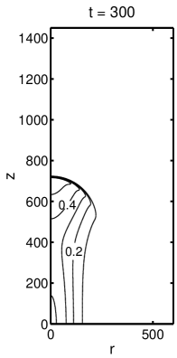
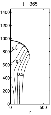
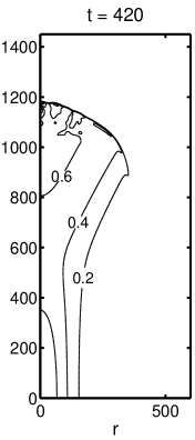
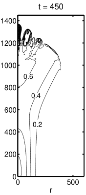
FIG. 1.: Evolution of spontaneous branching of anode directed streamers in a strong homogeneous background field at times $t=300$, 365, 420 and 450. Model, initial and boundary conditions are discussed in the text. The planar cathode is located at $z=0$ and the planar anode at $z=2000$ (shown is $0\leq z\leq 1400$). The radial coordinate extends from the origin up to $r=2000$ (shown is $0\leq r\leq 600$). The thin lines denote levels of equal electron density $\sigma$ with increments of 0.1 or 0.2 as indicated by the labels. The thick lines denote the higher electron density levels 1., 2., 3., 4., 5. and 6. These high densities appear only at the last time step $t=450$ in the core of the new branches.

We investigate the minimal streamer model, i.e., a “fluid approximation” with local field-dependent impact ionization reaction in a non-attaching gas like argon or nitrogen [2, 7, 8, 9, 10, 11, 12]. In detail, the dynamics is as follows:
(i) an impact ionization reaction in local field approximation: free electrons and positive ions are generated by impact of accelerated electrons on neutral molecules $\partial_{\tau}n_{e}+\nabla_{\bf R}\cdot{\bf j}_{e}=\partial_{\tau}n_{i}+\nabla_{\bf R}\cdot{\bf j}_{i}=|\mu_{e}{\cal E}n_{e}|\;\alpha_{0}\;\alpha(|{\cal E}|/E_{0})$; $n_{e,i}$ and ${\bf j}_{e,i}$ are particle densities or currents of electrons or ions, respectively, and ${\cal E}$ is the electric field; in all numerical work, we use the Townsend approximation $\alpha_{0}\;\alpha(|{\cal E}|/E_{0})=\alpha_{0}\;\exp(-E_{0}/|{\cal E}|)$ with parameters $\alpha_{0}$ and $E_{0}$ for the effective cross-section.
(ii) drift and diffusion of the charged particles in the local electric field ${\bf j}_{e}=-\mu_{e}{\cal E}n_{e}-D_{e}\nabla_{\bf R}n_{e}$, where in anode-directed streamers the mobility of the ions actually can be neglected because it is more than two orders of magnitude smaller than the mobility $\mu_{e}$ of the electrons, so ${\bf j}_{i}=0$,
(iii) the modification of the externally applied electric field through the space charges of the particles according to the Poisson equation $\nabla_{\bf R}\cdot{\cal E}=e(n_{i}-n_{e})/\epsilon_{0}$. It is this coupling between space charges and electric field which makes the problem nonlinear.

The natural units of the model are given by the ionization length $R_{0}=\alpha_{0}^{-1}$, the characteristic impact ionization field $E_{0}$, and the electron mobility $\mu_{e}$ determining the velocity $v_{0}=\mu_{e}E_{0}$ and the time scale $\tau_{0}=R_{0}/v_{0}$. Hence we introduce the dimensionless coordinates [12] ${\bf r}={\bf R}/R_{0}$ and $t=\tau/\tau_{0}$, the dimensionless field ${\bf E}={\bf{\cal E}}/E_{0}$, the dimensionless electron and ion particle densities $\sigma=n_{e}/n_{0}$ and $\rho=n_{i}/n_{0}$ with $n_{0}=\varepsilon_{0}E_{0}/(eR_{0})$, and the dimensionless diffusion constant $D=D_{e}/(R_{0}v_{0})$. After this rescaling, the model has the form:

$$\partial_{t}\;\sigma\;-\;\nabla\cdot\left(\sigma\;{\bf E}+D\;\nabla\sigma\right) = \sigma\;f(|{\bf E}|)~{},$$ (1)

$$\partial_{t}\;\rho\; = \sigma\;f(|{\bf E}|)~{},$$ (2)

$$\rho-\sigma = \nabla\cdot{\bf E}~{}~{},~{}~{}{\bf E}=-\nabla\Phi~{},$$ (3)

$$f(|{\bf E}|)=|{\bf E}|\;\alpha(|{\bf E}|)~{} \Big{(}= |{\bf E}|\;e^{-1/|{\bf E}|}~{}\mbox{in sim.}\Big{)}~{}.$$ (4)

In the simulations presented here, a planar cathode is located at $z=0$ and a planar anode at $z=2000$. The stationary potential difference between the electrodes $\Delta\Phi=1000$ corresponds to a uniform background field ${\bf E}=-0.5\;{\bf e}_{z}$ in the $z$ direction. For nitrogen under normal conditions with effective parameters as in [10, 11], this corresponds to an electrode separation of $\approx$ 5 mm and a potential difference of $\approx$ 50 kV. The unit of time $\tau_{0}$ is $\approx 3$ ps, and the unit of field $E_{0}$ is $\approx 200$ kV/cm. We used $D=0.1$ which is appropriate for nitrogen, and we assumed cylindrical symmetry of the streamer. The radial coordinate extends from the origin up to $r=2000$ to avoid lateral boundary effects on the field configuration. As initial condition, we used an electrically neutral Gaussian ionization seed on the cathode

$$\sigma(r,z,t=0)=\rho(r,z,t=0)=10^{-6}\;e^{-(z^{2}+r^{2})/100^{2}}.$$ (5)

The parameters of our numerical experiment are essentially the same as in the earlier simulations of Vitello et al. [11], except that our background electric field is twice as high; the earlier work had 25 kV applied over a gap of 5 mm. This corresponded to a dimensionless background field of 0.25, and branching was not observed.

In Fig. 1 we show the electron density levels at four time steps of the evolution in the higher background field of 0.5. We observe that at time $t=420$, the streamer develops instabilities at the tip. At time $t=450$, these instabilities have grown out into separate fingers. Because of the imposed cylindrical geometry, the further evolution after branching ceases to be physical. On the other hand, the main effect of the unphysical symmetry constraint is to suppress all linear instability modes that are not cylindrically symmetric. Hence in a fully 3D system, the instability will develop even earlier than here.

Further simulations show: $(a)$ branching does not occur in a system of the same size in the lower background field of 0.25, in agreement with [11]. $(b)$ Branching is not due to the proximity of the anode, since in a system with twice the electrode separation (with the anode at $z=4000$) and with twice the potential difference ($\Delta\Phi=2000$) — so with the same background field —, the streamer branches in about the same way after about the same time and travel distance. $(c)$ The phenomenon is not specific to the particular initial condition (5). $(d)$ Branching does somewhat depend on the numerical discretization. A wider numerical mesh leads to a higher effective noise level; and the branching then is triggered somewhat earlier. $(e)$ Occasionally, we observe a different tip splitting mode. In Fig. 1 at time $t=450$, the finger on the axis develops the strongest with $\sigma$ exceeding 6, while in the fingers off the axis, $\sigma$ stays below 3. In the other branching mode, the first finger off the axis outruns the finger on the axis.

Before we discuss the physical nature of the instability, we explain our numerical approach: we used uniform space-time grids with a spatial mesh of $1000\times 1000$. The spatial discretization is based on local mass balances. The diffusive fluxes are approximated in standard fashion with second order accuracy. For the convective fluxes a third order upwind-biased formula was chosen to reduce the numerical oscillations that are common with second order central fluxes. Such oscillations can be completely avoided, e.g., by flux-limiting, but preliminary tests showed that the upwind-biased formula already gives sufficient numerical monotonicity and is much faster. Time stepping is based on an explicit linear 2-step method, where at each time step the Poisson equation is solved by the FISHPACK routine. References for these procedures can be found in [14].

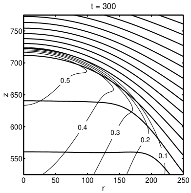
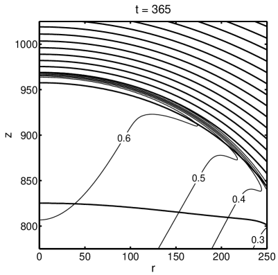
FIG. 2.: A zoom into the head of the streamer from Fig. 1 at the first two time steps. The aspect ratio is equal and the axis scaling identical at both times. The thin lines are the levels of equal electron density as in Fig. 1. The thick lines are electrical equipotential lines in steps of $\Delta\Phi=12$.

To understand now why and at which stage the streamer develops a tip splitting instability, in Fig. 2, we zoom into the streamer head. Shown are the first two time steps from Fig. 1 with the electron density levels again as thin lines, and additionally with the equipotential lines as thick lines. One observes that during the temporal evolution prior to branching, both the curvature and the thickness of the ionization front decrease. So the width of the front becomes much smaller than its radius of curvature, and an interface approximation becomes increasingly justified. The electric field inside the streamer head also decreases, so that the ionization front more and more coincides with an equipotential surface. In summary, the ionization front evolves towards a weakly curved and almost equipotential moving ionization boundary. At the same time, the electric field immediately ahead of the streamer increases.

We argue now that a transient stage of an approximately equipotential and weakly curved ionization boundary leads to tip splitting. Conversely, we argue that tip splitting in the lower background field of 0.25 is not observed within the presently and previously [11] investigated gap lengths because the transient stage of Fig. 2 is not reached before the streamer reaches the anode.

In fact, the streamer in Fig. 2 approaches the limit of “ideal conductivity”: the conducting body has $\Phi\approx{\rm const.}$, while in the non-ionized region $\nabla^{2}\Phi=0$ due to the absence of space charges. The boundary between the two regions moves approximately with the drift velocity $v_{f}\propto\nabla\Phi$ or with the diffusion corrected velocity $v_{f}\propto\nabla\Phi\;\left(1+2\sqrt{D\;\alpha(|\nabla\Phi|)/|\nabla\Phi|}\right)$ [12]. Our simulations are the first numerical evidence that the “ideal conductivity” limit can be approached within our model.

This limit of ideally conducting streamers in an electric field that becomes uniform far ahead of the front was studied by Lozansky and Firsov [7]. They realized that uniformly propagating paraboloids of arbitrary radius of curvature are solutions of this problem. They did not realize that these paraboloids are mathematically equivalent to the Ivantsov paraboloids [13] of dendritic growth found earlier. The uniformly propagating Ivantsov paraboloids in the early 80’ies were identified as dynamically unstable. This is generally the case for such so-called Laplacian growth problems without a regularization mechanism. Since ideally conducting streamers also pose such a Laplacian growth problem [12], the dynamical instability of the structure shown in Fig. 2 can be expected, and it actually occurs as can be seen in Fig. 1. This explains qualitatively why tip splitting occurs.

For a quantitative analysis, a system specific regularization mechanism has to be found [12, 13]. Its identification is intricate because negative streamer fronts are so-called pulled fronts whose dynamics is dominated by the leading edge rather than the nonlinear interior of the front [15]. Therefore standard methods like the pertubative derivation of a moving boundary approximation for the model (1)–(4) does not work [16]. (Pulling also implies that standard numerical methods with adaptive grids are inefficient.) However, the ionization front has two intrinsic length scales, a diffusion length and an electric screening length. We therefore explore the approximation of $D=0$. It is smooth for the velocity of negative fronts [12] and eliminates the leading edge, and hence suppresses the pulled nature of the front. Rather the front becomes a shock front for the electron density, while the intrinsic length scale of the electric screening layer behind the shock remains.

As a first step to understand the short wave length regularization of perturbations due to this screening length, we have investigated the transversal instability modes of a planar ionization front in the limit $D=0$ in a field that approaches the uniform limit ${\bf E}=-E_{\infty}\;{\bf e}_{z}$ far ahead of the front. The planar unperturbed front propagates with velocity $v=E_{\infty}$, which equals the drift velocity of the electrons precisely at the shock front. The implicit analytical front solution can be found in [12]. In a comoving frame $\xi=z-vt$, we denote it by $\big{(}\;\sigma_{0}(\xi),\rho_{0}(\xi),\Phi_{0}(\xi)\;\big{)}$. The Fourier components $\big{(}\;\tilde{\sigma}_{k},\tilde{\rho}_{k},\tilde{\Phi}_{k}\;\big{)}$ of a transversal linear perturbation are defined through

$$\sigma=\sigma_{0}(\xi)+\int dk\;\tilde{\sigma}_{k}(\xi)\;e^{ikx+st}+\ldots~{}~{}~{}\mbox{etc.}$$ (6)

For the derivation of the boundary conditions on the shock front, it is more convenient to write a single Fourier component as $\sigma=\sigma_{0}\left(\xi-e^{ikx+st}\right)+\sigma_{k}(\xi)\;e^{ikx+st}+\ldots$. With this ansatz and the auxiliary field $\psi_{k}=\partial_{\xi}\phi_{k}$, the Fourier components solve the inhomogeneous equation

$$\partial_{\xi}\left(\begin{array}[]{c}\sigma_{k}\\ \rho_{k}\\ \psi_{k}\\ \phi_{k}\end{array}\right)={\bf M}_{s,k}\cdot\left(\begin{array}[]{c}\sigma_{k}\\ \rho_{k}\\ \psi_{k}\\ \phi_{k}\end{array}\right)-\left(\begin{array}[]{c}s\;\partial_{\xi}\sigma_{0}/(v+E_{0})\\ s\;\partial_{\xi}\rho_{0}/v\\ E_{0}k^{2}\\ 0\end{array}\right),$$ (19)

(20)

$${\bf M}_{s,k}=\left(\begin{array}[]{cccc}\frac{s+2\sigma_{0}-f(E_{0})-\rho_{0}}{v+E_{0}}&\frac{-\sigma_{0}}{v+E_{0}}&\frac{\partial_{\xi}\sigma_{0}-\sigma_{0}f^{\prime}(E_{0})}{v+E_{0}}&0\\ -f(E_{0})/v&s/v&-\sigma_{0}f^{\prime}(E_{0})/v&0\\ 1&-1&0&k^{2}\\ 0&0&1&0\end{array}\right).$$ (25)

The boundary conditions at the shock $\xi=0$ can be obtained from the analytical solution in the non-ionized area, and from the boundedness of the charge densities:

$$\left(\begin{array}[]{c}\sigma_{k}\\ \rho_{k}\\ \psi_{k}\\ \phi_{k}\end{array}\right)\stackrel{{\scriptstyle\xi\uparrow 0}}{{\longrightarrow}}\left(\begin{array}[]{c}f^{\prime}(v)/(1+s/f(v))\\ 0\\ 1\\ (vk-s)/(sk)\end{array}\right).$$ (26)

The other boundary conditions are obtained by imposing that at $\xi\to-\infty$ the electric field decays and the densities become constant.

These equations together with the boundary conditions define an eigenvalue problem for $s=s(k,v)$ with $v=E_{\infty}$. It can be solved numerically by shooting from $\xi=0$ towards $-\infty$. In agreement with analytical limits — details will be given elsewhere —, we find

$$s(k) = \left\{\begin{array}[]{ll}|E_{\infty}|\;k&~{}~{}\mbox{ for }k\ll\alpha(|E_{\infty}|)/2\\ |E_{\infty}|\;\alpha(|E_{\infty}|)/2&~{}~{}\mbox{ for }k\gg\alpha(|E_{\infty}|)/2\end{array}\right..$$ (29)

This means that the electric screening length $1/\alpha(|E_{\infty}|)$ does regularize the instability of short wave length perturbations from linear growth in $k$ to the saturation value $s(k)=|E_{\infty}|\;\alpha(E_{\infty})/2$. A small positive growth rate remains, but the analytical derivation of (29) hints to the unconventional possibility that sufficiently curved fronts actually are stable to short wave length perturbations. This question is presently under investigation. If true, it would identify a most unstable wave length determining the width of the fingers that emerge after tip splitting.

In conclusion, we have presented numerical evidence that anode-directed streamers in a sufficiently strong, but uniform field can branch spontaneously even in a fully deterministic fluid model. We have argued that this happens when the streamer approaches the limit of ideal conductivity. We have established a qualitative mathematical analogy with tip splitting of viscous fingers through the concept of Laplacian growth, and we have analytically demonstrated that the electric screening length leads to an unconventional regularization. This opens the way to future quantitative analytical progress.

Acknowledgement: M.A. was supported by the EU-network “Patterns, Noise, and Chaos” and U.E. partially by the Dutch Science Foundation NWO.

REFERENCES

- [1] New address: Universidad Rey Juan Carlos, Escuela Superior de Ciencias Exp. y Tecnologia, c. Tulipan s/n, 28933 Mostoles, Madrid, Spain
- [2] Y.P. Raizer, Gas Discharge Physics (Springer, Berlin 1991).
- [3] E.M. van Veldhuizen (ed.): Electrical discharges for environmental purposes: fundamentals and applications (NOVA Science Publishers, New York 1999).
- [4] A.A. Kulikovsky, J. Phys. D: Appl. Phys. 33, 1514 (2000); and Phys. Rev. E 57, 7066 (1998).
- [5] L. Niemeyer, L. Pietronero, H.J. Wiesmann, Phys. Rev. Lett. 52, 1033 (1984); A.D.O. Bawagan, Chem Phys. Lett. 281 325 (1997).
- [6] H. Raether: Z. Phys. 112, 464 (1939) (in German).
- [7] E.D. Lozansky and O.B. Firsov, J. Phys. D: Appl. Phys. 6, 976 (1973).
- [8] M.I. D’yakonov, V.Y. Kachorovskii: Sov. Phys. JETP 67, 1049 (1988); and Sov. Phys. JETP 68, 1070 (1989).
- [9] E.M. Bazelyan, Yu.P. Raizer, Spark Discharges (CRS Press, New York, 1998); Yu.P. Raizer, A.N. Simakov, Plasma Phys. Rep. 24, 700 (1998).
- [10] S.K. Dhali and P.F. Williams, Phys. Rev. A 31, 1219 (1985) and J. Appl. Phys. 62, 4696 (1987).
- [11] P.A. Vitello, B.M. Penetrante, and J.N. Bardsley, Phys. Rev. E 49, 5574 (1994).
- [12] U. Ebert, W. van Saarloos and C. Caroli, Phys. Rev. Lett. 77, 4178 (1996); and Phys. Rev. E 55, 1530 (1997).
- [13] For a review and a collection of original articles, see P. Pelcé: Dynamics of Curved Fronts (Academic Press, San Diego 1988).
- [14] P. Wesseling, Principles of Computational Fluid Dynamics, Springer Series in Comp. Math. 29 (Berlin 2001).
- [15] U. Ebert and W. van Saarloos, Phys. Rev. Lett. 80, 1650 (1998); and Physica D 146, 1–99 (2000).
- [16] U. Ebert, W. van Saarloos, Phys. Rep. 337, 139 (2000).