Resonances and superlattice pattern
stabilization in two-frequency
forced Faraday waves

Abstract

We investigate the role weakly damped modes play in the selection of Faraday wave patterns forced with rationally-related frequency components $m\omega$ and $n\omega$. We use symmetry considerations to argue for the special importance of the weakly damped modes oscillating with twice the frequency of the critical mode, and those oscillating primarily with the “difference frequency” $|n-m|\omega$ and the “sum frequency” $(n+m)\omega$. We then perform a weakly nonlinear analysis using equations of Zhang and Viñals [1] which apply to small-amplitude waves on weakly inviscid, semi-infinite fluid layers. For weak damping and forcing and one-dimensional waves, we perform a perturbation expansion through fourth order which yields analytical expressions for onset parameters and the cubic bifurcation coefficient that determines wave amplitude as a function of forcing near onset. For stronger damping and forcing we numerically compute these same parameters, as well as the cubic cross-coupling coefficient for competing waves travelling at an angle $\theta$ relative to each other. The resonance effects predicted by symmetry are borne out in the perturbation results for one spatial dimension, and are supported by the numerical results in two dimensions. The difference frequency resonance plays a key role in stabilizing superlattice patterns of the SL-I type observed by Kudrolli, Pier and Gollub [2].

,

1 Introduction

The Faraday wave system provides the canonical example of how spatiotemporal patterns form through a parametric instability. In this system, a fluid subjected to a time-periodic vertical acceleration of sufficient strength undergoes an instability to standing waves on the free surface. In his original experiment [3] Faraday observed that the standing waves had half the frequency of the forcing; this is the familiar subharmonic response. Other experimentalists subsequently observed familiar patterns such as stripes, squares, and hexagons (see [4] for a review).

More recent experiments have utilized the two-frequency forcing function, which we may write in the following forms:

$$g(t) = g_{z}[\cos(\chi)\cos(m\omega t)+\sin(\chi)(n\omega t+\phi)]$$

$$= g_{m}\cos(m\omega t)+g_{n}(n\omega t+\phi)$$

$$= G_{m}\e^{im\omega t}+G_{n}\e^{in\omega t}+c.c.$$

Here m and n are co-prime integers, so that the forcing function is periodic with period $T=2\pi/\omega$. An interesting feature of this forcing function is that the primary instability leading to Faraday waves may be either harmonic or subharmonic (with respect to $T$) depending on the value of $\chi$ and the parities of $m$ and $n$. For instance, if the $\cos(m\omega t)$ component is dominant and if m is even (odd) then the bifurcation will be to harmonic (subharmonic) waves. This was demonstrated numerically by the linear stability analysis of Besson et al. [5]. For $m$ and $n$ not both odd, there is a codimension-two point in the $g_{z}$ - $\chi$ parameter space (or alternatively, in $g_{m}$ - $g_{n}$ space) at which harmonic and subharmonic instabilities occur simultaneously at different spatial wave numbers. The corresponding value $\chi=\chi_{bc}$ is called the “bicritical point”. Experiments performed near the bicritical point have produced exotic patterns, including triangles [6], quasipatterns [2, 7] and superlattice patterns [2, 8, 9, 10].

The term “superlattice pattern” refers to a periodic pattern that has spatial structure on more than one length scale – typically, a small scale structure and a large scale spatial periodicity. A wealth of recent experimental work has produced superlattice patterns. In addition to the Faraday experiments with two-frequency forcing mentioned above, superlattice patterns have been observed in nonlinear optical systems [11], in vertically vibrated Rayleigh-Bénard convection [12, 13], in Faraday waves with single frequency forcing at very low frequencies [14] and in granular layers forced with two frequencies [15]. The superlattice patterns come in a variety of types, and may be comprised of different numbers of critical modes having different spatial arrangement and temporal dependence.

We mention two types of superlattice patterns here. One type is called “superlattice two” or SL-II in [2]. Patterns of this type have been shown to arise in a spatial period-multiplying bifurcation from hexagons; see [16, 17] for a bifurcation analysis of these patterns. In contrast, “superlattice one” or SL-I patterns exist as primary branches bifurcating directly from the trivial solution [18]. For SL-I Faraday wave patterns, one of the length scales is set (approximately) by the dominant frequency component in (1). Curiously, the second length scale in the pattern is not set by the other forcing frequency. For instance, a numerical linear analysis using the parameters corresponding to the experimental SL-I pattern from [2] indicates that the two critical wave numbers are in a ratio of 1.22 at the bicritical point, but the ratio of the two length scales in the pattern is actually observed to be $\sqrt{7}\approx 2.65$. The identification of a mechanism for the selection of the second length scale is our motivation for this paper.

Many studies of Faraday wave pattern formation [1, 6, 7, 8, 9, 10, 14, 19, 20, 21, 22, 23] focus on the effect that resonant triad interactions have on the nonlinear pattern selection problem. The triads of spatially resonant modes satisfy $\mathbf{k}_{1}\pm\mathbf{k}_{2}=\mathbf{k_{3}}$, where $|\mathbf{k_{1}}|=|\mathbf{k_{2}}|$ is the wave number of one of the instabilities at the bicritical point, and $|\mathbf{k_{3}}|$ is the wave number of the other. In [24] temporal symmetry arguments were used to show that this triad interaction affects pattern selection on the subharmonic side of the bicritical point, but not on the harmonic side. In [25] it was shown that weakly damped harmonic modes not associated with the bicritical point can affect harmonic and subharmonic pattern selection. Explicit numerical calculations were performed to demonstrate that the presence of a weakly damped harmonic mode influences pattern selection by affecting the cubic cross-coupling coefficient in the bifurcation equations describing the dynamics of competing waves.

In this paper, too, our goal is to investigate the role weakly damped modes play in pattern selection. We use symmetry considerations to explain the special importance of particular weakly damped harmonic modes in terms of their contributions to cubic cross-coupling coefficients in the relevant bifurcation equations. Specifically, we find that the most important weakly damped modes are the temporal harmonic of the Faraday-unstable mode oscillating with dominant frequency $m\omega$, the “difference frequency mode” oscillating with dominant frequency $|m-n|\omega$, and the “sum frequency mode” oscillating with dominant frequency $(m+n)\omega$. (Here, we have assumed without loss of generality that the $cos(m\omega t)$ component in (1) is the dominant one. Additionally, we exclude the forcing frequency ratios $m/n$ or $n/m$ equal to $1/2$, $1/3$, $1/4$, and $2/3$, in which case strong resonances are possible). Our symmetry arguments are borne out in a weakly nonlinear analysis that uses equations of Zhang and Viñals [1] which apply to weakly inviscid, semi-infinite fluid layers. For weak damping and forcing and one-dimensional waves, we perform a perturbation expansion through fourth order which yields analytical expressions for onset parameters and the cubic self-interaction coefficient that determines wave amplitude as a function of forcing amplitude near onset. For stronger damping and forcing we compute these same parameters numerically as well as the cubic cross-coupling coefficient $B(\theta)$ for competing waves travelling at an angle $\theta$ relative to each other. From the resulting analytical expressions for the one-dimensional case, we are able to quantify the effect of the key resonances and see how their existence depends on the forcing frequency ratio $m/n$. For the two dimensional case, our numerical results show that the resonance effects follow the same scaling laws as in the 1-d case. A simple argument, valid for weak damping and forcing which relies only on the inviscid dispersion relation, allows us to predict the spatial angles at which the resonances occur, and to see how their existence depends on $m$, $n$ and a dimensionless fluid gravity-capillarity parameter. A bifurcation analysis reveals that the difference frequency resonance can help stabilize an SL-I pattern whose large-scale periodicity depends on the wavelength associated with the difference frequency mode. We note that the difference frequency mode has been observed to play an important role in experiments where other complex Faraday wave patterns are formed [8, 9, 10].

This paper is organized as follows. In section 2.1 we review basic ideas about resonant triad interactions and their potential for affecting SL-I pattern selection. In section 2.2 we use symmetry arguments to identify which weakly damped modes we expect to be most important in terms of their contributions to the cross-coupling coefficient $B(\theta)$. Section 3 contains the weakly nonlinear analysis of the Zhang-Viñals equations for weak damping and forcing and one-dimensional waves, which leads to approximate formulas for the critical forcing and wave number, and the cubic self-interaction coefficient. The perturbation results for onset parameters are discussed in 4.1. The expression for the self-interaction coefficient and numerical results for the cross-coupling coefficient are examined in sections 4.2.1 and 4.2.2 respectively, with special attention given to the role played by resonant triads and the implications for SL-I pattern selection. We summarize our main results in section 5.

2 Background

2.1 Resonant triads, standing wave equations and pattern stability

For Faraday waves on a domain of infinite horizontal extent there is no preferred direction, so each wave number is associated with a circle of wave vectors in Fourier space. One of the simplest mechanisms through which waves on two different Fourier circles may interact is a resonant triad interaction. Such resonant triads consist of three wave vectors that determine an associated angle $\theta_{r}\in(0,\frac{\pi}{2}]$.

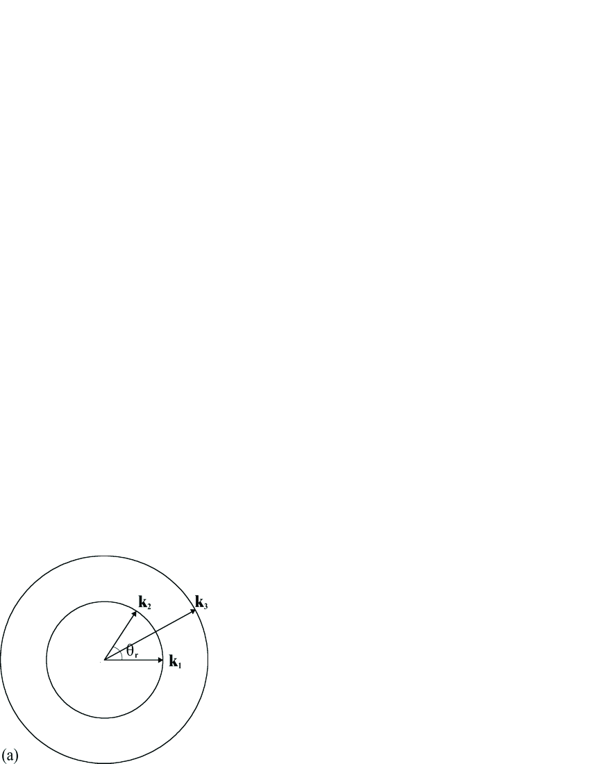
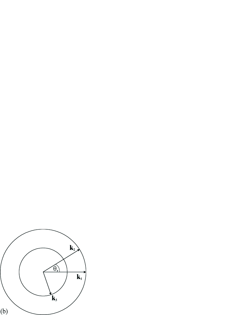
Figure 1: Spatially resonant triads of three wave vectors and their associated resonant angle $\theta_{r}$. (a) $\mathbf{k}_{1}+\mathbf{k}_{2}=\mathbf{k}_{3}$. (b) $\mathbf{k}_{1}-\mathbf{k}_{2}=\mathbf{k}_{3}$.

Two examples of spatially resonant triads are shown in figure 1. In figure 1a, the spatial resonance condition is

$$\mathbf{k}_{1}+\mathbf{k}_{2}=\mathbf{k}_{3}.$$ (2)

Here, $\mathbf{k}_{1}$ and $\mathbf{k}_{2}$ are wave vectors associated with neutrally stable modes of the Faraday instability, so that $\left|\mathbf{k}_{1}\right|=\left|\mathbf{k}_{2}\right|=k_{c}.$ The wave vector $|\mathbf{k}_{3}|$ is associated with a damped harmonic mode. The resonant angle $\theta_{r}$ satisfies

$$\cos\left(\frac{\theta_{r}}{2}\right)=\frac{|\mathbf{k}_{3}|}{2|\mathbf{k}_{1}|}.$$ (3)

For this resonant triad, $\sqrt{2}|\mathbf{k}_{1}|\leq|\mathbf{k}_{3}|\leq 2$. It is also possible to have a resonant triad where $0<|\mathbf{k}_{3}|\leq\sqrt{2}|\mathbf{k}_{1}|$; see figure 1b. Here, the spatial resonance condition is

$$\mathbf{k}_{1}-\mathbf{k}_{2}=\mathbf{k}_{3}.$$ (4)

and the resonant angle $\theta_{r}$ satisfies

$$\sin\left(\frac{\theta_{r}}{2}\right)=\frac{|\mathbf{k}_{3}|}{2|\mathbf{k}_{1}|}.$$ (5)

We follow [24, 25] and consider equations describing the slowly-varying amplitudes of the modes with wave vectors $\mathbf{k_{1}}\ldots\mathbf{k_{3}}$, which we assume satisfy the spatial resonance condition (2) (the case for (4) is similar):

$$\dot{Z_{1}} = \Lambda_{1}Z_{1}+\alpha_{1}\overline{Z}_{2}Z_{3}+(A|Z_{1}|^{2}+b|Z_{2}|^{2}+C|Z_{3}|^{2})Z_{1}$$ (6)

$$\dot{Z_{2}} = \Lambda_{1}Z_{2}+\alpha_{1}\overline{Z}_{1}Z_{3}+(A|Z_{2}|^{2}+b|Z_{1}|^{2}+C|Z_{3}|^{2})Z_{2}$$

$$\dot{Z_{3}} = \Lambda_{2}Z_{3}+\alpha_{2}Z_{1}Z_{2}+(D|Z_{1}|^{2}+D|Z_{2}|^{2}+E|Z_{3}|^{2})Z_{3}.$$

Here $Z_{1}$, $Z_{2}$, and $Z_{3}$ are the slowly varying amplitudes of the Fourier modes with wave vectors $\mathbf{k}_{1}$, $\mathbf{k}_{2}$, and $\mathbf{k}_{3}$ respectively, and the dot represents differentiation with respect to the slow time scale. All coefficients are real-valued. If the $Z_{3}$ mode is in fact damped (i.e. $\Lambda_{2}<0$) and the $Z_{1}$ and $Z_{2}$ modes are neutrally stable (i.e. $\Lambda_{1}=0$) then a further center manifold reduction may be performed to the critical $Z_{1}$ and $Z_{2}$ modes. Then $Z_{3}$ satisfies

$$Z_{3}=-\frac{\alpha_{2}}{\Lambda_{2}}Z_{1}Z_{2}+\ldots,$$ (7)

and the (unfolded) bifurcation problem, to cubic order, is

$$\frac{dZ_{1}}{dT} = \Lambda_{1}Z_{1}+A|Z_{1}|^{2}Z_{1}+B(\theta_{r})|Z_{2}|^{2}Z_{1}$$ (8)

$$\frac{dZ_{2}}{dT} = \Lambda_{1}Z_{2}+A|Z_{2}|^{2}Z_{2}+B(\theta_{r})|Z_{1}|^{2}Z_{2},$$

where

$$B(\theta_{r})=b-\frac{\alpha_{1}\alpha_{2}}{\Lambda_{2}}.$$ (9)

The dependence on the resonant angle $\theta_{r}$ indicates that the cross-coupling coefficient $B(\theta)$ for competing waves travelling at an angle $\theta$ relative to each other is evaluated at the angle of spatial resonance.

For appropriately chosen angles $\theta_{r}$, the bifurcation problem (8) describes dynamics on an invariant subspace of the twelve-dimensional problem which describes the competition of simple rolls, simple hexagons, certain rhombic patterns, and SL-I patterns. We are ultimately concerned with the cross-coupling coefficient $B(\theta)$, which plays a key role in determining the relative stability of these patterns. In particular, the stability properties of SL-I patterns with characteristic angles $\theta_{h}$ are enhanced when $B(\theta_{h})$ is small in magnitude; see [25] for a detailed discussion.

In [26], symmetry arguments are used to derive a scaling law for the quadratic coefficients $\alpha_{1}$ and $\alpha_{2}$ in (6) when the resonant triad applies to the bicritical point, and for the case of weak damping and forcing. For instance, it is shown that for $m$ odd and $n$ even, and for the case that the $\cos(m\omega t)$ forcing frequency component dominates, $\alpha_{1}$ and $\alpha_{2}$ are each proportional to $g_{m}^{\frac{n-2}{2}}g_{n}^{\frac{m-1}{2}}$. Thus depending on $m$ and $n$, the quadratic terms in (6) can be quite small. Its contribution to the pattern selection problem can only be made significant by getting sufficiently close to the bicritical point where $\Lambda_{2}\rightarrow 0$.

Here we will focus on resonant triads other than those associated with the bicritical point. In particular, we will identify resonant triads for which the quadratic terms scale (at most) linearly with $g$, i.e. the scaling is independent of $m$ and $n$. Thus, we expect these triads to play a more important role in pattern formation, at least away from the bicritical point and for weakly forced waves.

2.2 Determination of important resonances for weak damping and forcing

Our goal in this section is to examine resonant triads from a symmetry perspective with a special emphasis on temporal symmetries. Without loss of generality, we assume (unless otherwise specified) that the $\cos(m\omega t)$ forcing is of greater significance than the $\cos(n\omega t)$ forcing. For weak damping, the critical Faraday waves oscillate with a dominant frequency component of $m\omega/2$. We also consider weakly damped waves of frequency $\Omega>0$ $(\Omega\neq m\omega/2)$, to be determined such that they lead to the largest possible contribution to the cross-coupling coefficient $B(\theta)$ when slaved away; cf. (7) - (9) in section 2.1. Strong resonances are possible when the forcing frequency ratio $m/n$ or $n/m$ is equal to $1/2$, $1/3$, $1/4$, and $2/3$; we exclude these cases from our analysis.

We follow [26] and focus on travelling waves, for which the action of time-translation is transparent. The travelling wave bifurcation equations are then reduced to those describing the standing wave problem. Specifically, we expand the fluid surface height $h(\mathbf{x},t)$, $\mathbf{x}\in\mathbb{R}^{2}$, in terms of the following six travelling waves:

$$z_{1}\e^{i(\mathbf{k}_{1}\cdot\mathbf{x}+\frac{1}{2}m\omega t)}+w_{1}\e^{i(\mathbf{k}_{1}\cdot\mathbf{x}-\frac{1}{2}m\omega t)}+z_{2}\e^{i(\mathbf{k}_{2}\cdot\mathbf{x}+\frac{1}{2}m\omega t)}$$ (10)

$$\mbox{}+w_{2}\e^{i(\mathbf{k}_{2}\cdot\mathbf{x}-\frac{1}{2}m\omega t)}+z_{3}\e^{i(\mathbf{k}_{3}\cdot\mathbf{x}+\Omega t)}+w_{3}\e^{i(\mathbf{k}_{3}\cdot\mathbf{x}-\Omega t)}+\ c.c.$$

Here, $z_{j}$ and $w_{j}$, $j=1,2,3$, are the slowly varying amplitudes of the travelling waves. The wave vectors $\mathbf{k}_{1}\ldots\mathbf{k_{3}}$ are assumed to satisfy the spatial resonance condition (2) (the argument for (4) is similar). The frequency $\Omega$ and the wave number $|\mathbf{k}_{3}|$ are related by a dispersion relation. In writing (10) we have assumed the problem is posed on an unbounded horizontal domain and then restricted our attention to solutions that are periodic on a rhombic lattice. Spatial translation symmetry acts on $(z_{j},w_{j})$, $j=1,2,3$, as

$$\mathrm{T}(\Theta_{1},\Theta_{2}):(z_{j},w_{j})\rightarrow(z_{j},w_{j})\e^{i\Theta_{j}},\quad\Theta_{3}\equiv\Theta_{1}+\Theta_{2}$$ (11)

where $(\Theta_{1},\Theta_{2})\in\mathrm{T}^{2}$. A rotation by $\pi$, denoted by $R$, acts as

$$\mathcal{R}:(z_{j},w_{j})\rightarrow(\overline{w}_{j},\overline{z}_{j}),\quad j=1,2,3.$$ (12)

and a reflection in the plane containing $\mathbf{k}_{3}$, denoted by $\kappa$, acts as

$$\mathcal{\kappa}:(z_{1},w_{1}) \leftrightarrow (z_{2},w_{2})$$ (13)

$$(z_{3},w_{3}) \rightarrow (z_{3},w_{3}).$$

Furthermore, there is a time-translation symmetry which acts on the forcing parameters in (1) and on the complex travelling wave amplitudes in (10):

$$\mathrm{T}_{\Delta t}:(z_{1},z_{2},z_{3}) \rightarrow (z_{1}\e^{i\frac{1}{2}m\omega\Delta t},z_{2}\e^{i\frac{1}{2}m\omega\Delta t},z_{3}\e^{i\Omega\Delta t})$$ (14)

$$(w_{1},w_{2},w_{3}) \rightarrow (w_{1}\e^{-i\frac{1}{2}m\omega\Delta t},w_{2}\e^{-i\frac{1}{2}m\omega\Delta t},w_{3}\e^{-i\Omega\Delta t})$$

$$(G_{m},G_{n}) \rightarrow (G_{m}\e^{im\omega\Delta t},G_{n}\e^{in\omega\Delta t}).$$

We now determine which quadratic terms will be allowed in the travelling wave amplitude equations, anticipating that these terms will lead to contributions to $B(\theta)$. For example, from the spatial translation symmetry (11), the only quadratic terms that are allowed in the $\dot{z}_{1}$ equation are $\overline{z}_{2}z_{3}$, $\overline{z}_{2}w_{3}$, $\overline{w}_{2}z_{3}$ and $\overline{w}_{2}w_{3}$.

We now consider the restrictions placed by the time translation symmetry (14) in order to determine which $\Omega$ are allowed. We expect the largest contributions to $B(\theta)$ in (8) to occur when the coefficients of quadratic terms are independent of the forcing amplitudes $G_{m}$ and $G_{n}$ at leading order, at least for small forcing. In this case, there is only one quadratic term that is permitted, namely

1. $\overline{w}_{2}w_{3}$ with $\Omega=m\omega$.

The next largest contributions to $B(\theta)$ occur when the coefficients of the quadratic terms in (6) are proportional to one power of $G_{m}$ or $G_{n}$ at leading order. In this case, the permitted equivariant terms in the $\dot{z}_{1}$ equation are

1. $\overline{G}_{m}\overline{z}_{2}z_{3}$ with $\Omega=2m\omega$

2. $G_{n}\overline{z}_{2}z_{3}$ with $\Omega=(m-n)\omega$ if $m>n$

3. $G_{n}\overline{z}_{2}w_{3}$ with $\Omega=(n-m)\omega$ if $n>m$

4. $\overline{G}_{n}\overline{z}_{2}z_{3}$ with $\Omega=(m+n)\omega$

5. $\overline{G}_{n}\overline{w}_{2}z_{3}$ and $G_{n}\overline{w}_{2}w_{3}$ with $\Omega=n\omega$.

We may immediately dispense with several of these cases. The resonance in case ii. is not relevant for our investigation of Faraday waves because the weakly damped mode oscillating with frequency $2m\omega$ is at sufficiently high wave number that the spatial resonance condition (2) cannot be satisfied for the inviscid dispersion relation. The resonance in case v. does not result in a contribution to $B(\theta)$ at linear order in $G_{m}$, $G_{n}$. This may be understood by considering the effects of an approximate time reversal symmetry and an approximate Hamiltonian structure [27] and has been verified by an explicit perturbation calculation similar to those performed in section 3.

We refer to iiia. and iiib. as cases of “difference frequency resonance.” We now examine the amplitude equations for case iiia. (case iiib. is analogous) which are determined by the symmetries (11) - (14). The cubic truncation takes the form

$$\dot{z_{1}} = \lambda_{1}z_{1}+\delta G_{m}w_{1}+G_{n}\beta_{1}\overline{z}_{2}z_{3}+r_{0}w_{1}z_{2}\overline{w}_{2}$$

$$\mbox{}+(r_{1}|z_{1}|^{2}+r_{2}|z_{2}|^{2}+r_{3}|z_{3}|^{2}+r_{4}|w_{1}|^{2}+r_{5}|w_{2}|^{2}+r_{6}|w_{3}|^{2})z_{1}$$

$$\dot{z_{3}} = \lambda_{2}z_{3}+\overline{G}_{n}\beta_{2}z_{1}z_{2}$$

$$\mbox{}+(r_{7}|z_{1}|^{2}+r_{7}|z_{2}|^{2}+r_{8}|z_{3}|^{2}+r_{9}|w_{1}|^{2}+r_{9}|w_{2}|^{2}+r_{10}|w_{3}|^{2})z_{3}.$$

Related equations for $\dot{z_{2}}$, $\dot{w_{1}}$, $\dot{w_{2}}$, and $\dot{w_{3}}$ can be obtained from the discrete spatial symmetries (12) and (13). The $\delta G_{m}w_{1}$ term in (2.2) is the usual parametric forcing term. We have dropped linear and quadratic terms that scale higher than linearly in $G_{m}$ and $G_{n}$. We have also dropped any cubic terms whose coefficients depend on these parameters.

Since the resonant $z_{3}$ mode is damped ($\lambda_{2}<0$), we may slave it away so that (2.2) becomes

$$\dot{z_{1}} = \lambda_{1}z_{1}+\delta G_{m}w_{1}+r_{0}w_{1}z_{2}\overline{w}_{2}$$

$$\mbox{}+\left\{r_{1}|z_{1}|^{2}+\left(r_{2}-\frac{|G_{n}|^{2}\beta_{1}\beta_{2}}{\lambda_{2}}\right)|z_{2}|^{2}+r_{4}|w_{1}|^{2}+r_{5}|w_{2}|^{2}\right\}z_{1}.$$

and equations related by the discrete spatial symmetries (12) and (13).

For sufficiently large forcing $|G_{m}|$, the trivial solution of (2.2) loses stability. A center manifold reduction to standing waves equations of the form (8) may be formed at the critical forcing strength. The cross-coupling coefficient $B(\theta)$ in (8) then includes a contribution proportional to $|G_{n}|^{2}/(\mathop{\mathrm{Re}}\lambda_{2})$ that results from slaving the difference frequency mode.

Similar arguments can be made for case iv., in which the resonant mode oscillates at the so-called “sum frequency” $(m+n)\omega$. For this case, too, the slaved mode results in a contribution to $B(\theta)$ that is proportional to $|G_{n}|^{2}/(\mathop{\mathrm{Re}}\lambda)$, where $\mathop{\mathrm{Re}}\lambda$ represents the damping of the slaved resonant mode.

Case i. corresponds to the well-known 1:2 temporal resonance, which is present for single frequency forcing [1]. An analysis similar to that performed above reveals that slaving of the damped mode oscillating with dominant frequency $m\omega$ results in a contribution to $B(\theta)$ which is independent of $G_{m}$ and $G_{n}$, and is inversely proportional to $\mathop{\mathrm{Re}}(\lambda)$. Thus we expect that this contribution will be larger than that due to the sum or difference frequency resonances.

For weak damping and forcing, then, we expect the standing wave modes with frequency $m\omega$, $|m-n|\omega$, and $(m+n)\omega$ to be the most important weakly damped modes in terms of their contributions to $B(\theta)$. Due to the constraints imposed by temporal symmetries, any other resonant modes will necessarily have higher powers of $g$ in front of the quadratic terms in their travelling wave equations, and thus will result in smaller contributions to $B(\theta)$ for weak forcing. The exception is the wave oscillating with dominant frequency $\frac{1}{2}n\omega$. Because this bifurcates directly from the bicritical point, its damping may be made arbitrarily small for appropriately chosen parameters, and its slaving can result in a large contribution to $B(\theta)$ as demonstrated in [25]. Since our analysis assumes that the resonant modes have finite damping (i.e. we are bounded away from the bicritical point), this case is excluded here.

3 Perturbation analysis for one dimensional waves

Using the ideas discussed in the previous section, we now perform a perturbation analysis on the Zhang-Viñals Faraday wave equations (which we introduce in section 3.1) to obtain quantitative results for Faraday waves in one spatial dimension. The forcing frequency ratios $m/n$ or $n/m$ equal to $1/2$, $1/3$, $1/4$, and $2/3$ are special cases of strong resonance which we exclude from our analysis.

Since there is no spatial angle $\theta$ to tune in one dimension, the 1:2 spatial resonance is the only possibility for the modes depicted in figure 1. For the one-dimensional case, then, a resonant triad interaction occurs when a standing wave with critical wave number $k$ and its spatial harmonic with wave number $2k$ fulfill one of the temporal resonance conditions from section 2.2. This situation may be achieved by varying fluid parameters in the dispersion relation. In particular, in our calculations we vary a dimensionless capillarity parameter. Near those special values of the capillarity parameter where a temporal resonance occurs, we expect additional contributions to the cubic self-interaction coefficient $A$ in the standing wave bifurcation equation

$$\frac{dZ_{1}}{dT}=\Lambda_{1}Z_{1}+A|Z_{1}|^{2}Z_{1},$$ (18)

which is simply (8) restricted to one spatial dimension.

3.1 The Zhang-Viñals Hydrodynamic Equations

Zhang and Viñals derive from the Navier Stokes equations reduced equations for Faraday waves in [1]. This derivation is accomplished by focusing on fluids of low viscosity and making a quasipotential approximation. The resulting equations apply to weakly damped, small amplitude surface waves on a semi-infinite layer of fluid. The system consists of two evolution equations for the surface height $h(\mathbf{x},\tau)$ and surface velocity potential $\Phi(\mathbf{x},\tau)$, where $\mathbf{x}\in\mathbb{R}^{2}$ is the horizontal coordinate. We assume periodic boundary conditions.

The Zhang-Viñals equations are

$$(\partial_{\tau}-\gamma\nabla^{2})h-\mathop{\widehat{\mathcal{D}}}\Phi = \mathcal{F}(h,\Phi)$$ (19)

$$(\partial_{\tau}-\gamma\nabla^{2})\Phi-\left(\Gamma_{0}\nabla^{2}-G(\tau)\right)h = \mathcal{G}(h,\Phi),$$ (20)

where the nonlinear terms are

$$\mathcal{F}(h,\Phi) = -\nabla\cdot(h\nabla\Phi)+\frac{1}{2}\nabla^{2}(h^{2}\mathop{\widehat{\mathcal{D}}}\Phi)-\mathop{\widehat{\mathcal{D}}}(h\mathop{\widehat{\mathcal{D}}}\Phi)$$

$$\mbox{}+\mathop{\widehat{\mathcal{D}}}\left\{h\mathop{\widehat{\mathcal{D}}}(h\mathop{\widehat{\mathcal{D}}}\Phi)+{1\over 2}h^{2}\nabla^{2}{\Phi}\right\}$$

$$\mathcal{G}(h,\Phi) = {1\over 2}(\widehat{D}\Phi)^{2}-{1\over 2}(\nabla\Phi)^{2}-(\widehat{\mathcal{D}}\Phi)\left\{h\nabla^{2}\Phi+\mathop{\widehat{\mathcal{D}}}(h\widehat{\mathcal{D}}\Phi)\right\}$$

$$\mbox{}-{1\over 2}\Gamma_{0}\nabla\cdot\left\{(\nabla h)(\nabla h)^{2}\right\}.$$

(For brevity, we drop the $h$ and $\Phi$ dependence of $\mathcal{F}$ and $\mathcal{G}$ from now on.) The operator $\mathop{\widehat{\mathcal{D}}}$ is a nonlocal operator that multiplies each Fourier component of a field by its wave number, e.g. $\mathop{\widehat{\mathcal{D}}}e^{i{\bf k}\cdot{\bf x}}=|{\bf k}|e^{i{\bf k}\cdot{\bf x}}$. Here time has been scaled by $\omega$ so that the dimensionless two-frequency acceleration is

$$G(\tau) = G_{0}-\left[f_{m}\cos(m\tau)+f_{n}\cos(n\tau+\phi)\right]$$

$$= G_{0}-f\left[\cos(\chi)\cos(m\tau)+\sin(\chi)\cos(n\tau+\phi)\right].$$

The damping number ($\gamma$), capillarity number ($\Gamma_{0}$), gravity number ($G_{0}$), and dimensionless accelerations ($f_{m}$ and $f_{n}$) are related to the forcing function (3.1) and the fluid parameters by

$$\gamma\equiv{2\nu\widetilde{k}^{2}\over\omega},\quad\Gamma_{0}\equiv{\Gamma\widetilde{k}^{3}\over\rho\omega^{2}},\quad G_{0}\equiv{g_{0}\widetilde{k}\over\omega^{2}},\quad f_{m}\equiv{g_{m}\widetilde{k}\over\omega^{2}},\quad f_{n}\equiv{g_{n}\widetilde{k}\over\omega^{2}}.$$ (24)

Here $\nu$ is the kinematic viscosity, $\Gamma$ is the surface tension, $\rho$ is the fluid density, and the wave number $\widetilde{k}$ is chosen to satisfy the gravity-capillary wave dispersion relation

$$g_{0}\widetilde{k}+{\Gamma\widetilde{k}^{3}\over\rho}=\Bigl{(}{m\omega\over 2}\Bigr{)}^{2}.$$ (25)

Note that (24) and (25) imply a relationship between the gravity number and the capillarity number, namely

$$G_{0}+\Gamma_{0}=\frac{m^{2}}{4}.$$ (26)

Following [24], we express the governing equations in the following alternative form. We apply $(\partial_{\tau}-\gamma\nabla^{2})$ to (19) to obtain

$$(\partial_{\tau}-\gamma\nabla^{2})^{2}h-(\partial_{\tau}-\gamma\nabla^{2})\mathop{\widehat{\mathcal{D}}}\Phi=(\partial_{\tau}-\gamma\nabla^{2})\mathcal{F}.$$ (27)

In (27), we substitute for $(\partial_{\tau}-\gamma\nabla^{2})\Phi$ by using (20). The resulting equation and equation (19) (which we rearrange) constitute the system of equations that we use in our perturbation analysis:

$$\left\{(\partial_{\tau}-\gamma\nabla^{2})^{2}-\mathop{\widehat{\mathcal{D}}}\left[\Gamma_{0}\nabla^{2}-G(\tau)\right]\right\}h = (\partial_{\tau}-\gamma\nabla^{2})\mathcal{F}+\mathop{\widehat{\mathcal{D}}}\mathcal{G}$$ (28)

$$\mathop{\widehat{\mathcal{D}}}\Phi = (\partial_{\tau}-\gamma\nabla^{2})h-\mathcal{F}.$$ (29)

3.2 Outline of the calculation

We calculate from the Zhang-Viñals equations (28) - (29) systems of ODEs for travelling waves in one spatial dimension that are valid for the different cases of spatiotemporal resonance described in section 2.2. Our perturbation calculations are performed for small amplitude waves in the limit of weak damping and forcing ($\gamma,f_{m},f_{n}\ll 1$).

For our calculations, we focus on counter-propagating travelling waves having critical wave number $k$ (to be determined) which are assumed to be subharmonic to the dominant forcing component $\cos(m\tau)$ and thus, to leading order, have frequency $m/2$. We refer to these waves as the “basic waves”. Furthermore, we insist that $f_{n}$ not exceed the critical value at which standing waves of dominant frequency $n/2$ bifurcate. Thus, we do not include these waves in our nonlinear calculation, and our nonlinear analysis is restricted to the parameter region

$$0<f_{m}\ll 1,\quad 0<f_{n}<f_{n}^{crit.}\ll 1$$ (30)

which is bounded away from the bicritical point.

To facilitate our analysis, we perform four separate calculations, each of which pertains to a different possible case of spatiotemporal resonance. The first case is a nonresonant case, for which we retain only the basic waves in the leading order solution of the perturbation problem. Then we consider cases in which the basic waves are (nearly) temporally resonant with their spatial harmonics having wave number $2k$. Based on the arguments in section 2, the three resonant frequencies we consider are $m$ (1:2 temporal resonance), $|m-n|$ (difference frequency resonance) and $m+n$ (sum frequency resonance). Each resonance may be achieved by choosing a particular value of the capillarity parameter $\Gamma_{0}$. For each of these resonant cases, we retain both the basic waves and the resonant waves at leading order. For all cases, resonant terms at subsequent orders in the perturbation calculation lead to solvability conditions, from which we obtain travelling wave amplitude equations, and by a further center manifold reduction, standing wave amplitude equations.

3.3 No resonance

We use the following scaling:

$$\gamma=\epsilon\gamma_{1},\quad f_{n}=\epsilon f_{n}^{1},\quad f_{m}=\epsilon f_{m}^{1}+\epsilon^{3}f_{m}^{3}+\ldots$$ (31)

$$k=k_{0}+\epsilon^{2}k_{2}+\ldots,\quad\partial_{\tau}\rightarrow\partial_{\tau}+\epsilon\partial_{\mathcal{T}_{1}}+\epsilon^{2}\partial_{\mathcal{T}_{2}}+\epsilon^{3}\partial_{\mathcal{T}_{3}}+\ldots$$

$$h=\epsilon h_{1}+\epsilon^{2}h_{2}+\epsilon^{3}h_{3}+\ldots,\quad\Phi=\epsilon\Phi_{1}+\epsilon^{2}\Phi_{2}+\epsilon^{3}\Phi_{3}+\ldots$$

where $0<\epsilon\ll 1$. The fields $h$ and $\Phi$ are functions of the spatial variable $x$, the fast time $\tau$, and the slow times $\mathcal{T}_{j}$.

The expressions for $f_{m}$ and $k$ indicate expansions of the critical wave number and forcing value. We find that terms proportional to $\epsilon^{2}$ in $f_{m}$ and $\epsilon$ in $k$ are not necessary. The wave number, forcing, time derivative, and the two fields are expanded through $\mathcal{O}(\epsilon^{3})$ because we carry out the perturbation calculation to $\mathcal{O}(\epsilon^{4})$. This higher order calculation is needed since $A$, the cubic coefficient in the standing wave equation (18), turns out to be an $\mathcal{O}(\epsilon)$ quantity. (This is related to a weakly broken time reversal symmetry as discussed in [26].)

At $\mathcal{O}(\epsilon)$, (28) is

$$\mathcal{L}_{0}h_{1}=0$$ (32)

where

$$\mathcal{L}_{0}\equiv\partial_{\tau}^{2}+\mathop{\widehat{\mathcal{D}}}(G_{0}-\Gamma_{0}\partial_{x}^{2}).$$ (33)

Equation (32) has an infinite-dimensional solution space consisting of all plane waves $\e^{ik_{0}x+i\Omega(k_{0})\tau}$ that satisfy the dispersion relation

$$\Omega^{2}(k_{0})=G_{0}k_{0}+\Gamma_{0}k_{0}^{3}.$$ (34)

Thus, $h_{1}$ should consist of a superposition of these plane waves, i.e. $h_{1}=\sum_{k_{0}}z(k_{0})\e^{ik_{0}x+i\Omega(k_{0})\tau}$, where the wave number $k_{0}$ may be any wave number that fits into our periodic domain. However, at $\mathcal{O}(\epsilon^{2})$, all of the amplitudes $z(k_{0})$ are damped on the slow time scales, except for the case $\Omega(k_{0})=m/2$, $k_{0}=1$. Using this a posteriori justification, we choose $h_{1}$ to include only those solutions which may grow on the slow time scales. Therefore, $h_{1}$ consists of one set of counter-propagating waves:

$$h_{1}=z_{1}\e^{ikx+i\frac{m}{2}\tau}+w_{1}\e^{ikx-i\frac{m}{2}\tau}+\ c.c.$$ (35)

where $z_{1}$ and $w_{1}$ are functions of $\mathcal{T}_{1}$, $\mathcal{T}_{2}$, and $\mathcal{T}_{3}$.

At $\mathcal{O}(\epsilon^{2})$, $\mathcal{O}(\epsilon^{3})$ and $\mathcal{O}(\epsilon^{4})$ we apply solvability conditions which yield the respective equations

$$\frac{\partial z_{1}}{\partial\mathcal{T}_{1}} = -\gamma_{1}z_{1}+i\eta_{1}w_{1}$$ (36)

$$\frac{\partial z_{1}}{\partial\mathcal{T}_{2}} = i\nu_{2}z_{1}+ic_{1}|z_{1}|^{2}z_{1}+ic_{2}|w_{1}|^{2}z_{1}$$ (37)

$$\frac{\partial z_{1}}{\partial\mathcal{T}_{3}} = -\gamma_{3}z_{1}+i\eta_{3}w_{1}+c_{3}|z_{1}|^{2}z_{1}+c_{4}|w_{1}|^{2}z_{1}$$

$$\mbox{}+ic_{5}|w_{1}|^{2}z_{1}+ic_{6}|w_{1}|^{2}w_{1}+ic_{7}z_{1}^{2}\overline{w}_{1}$$

and similar equations for $w_{1}$ which are related by the spatial reflection symmetry

$$x\rightarrow-x:\ (z_{1},w_{1})\rightarrow(\overline{w}_{1},\overline{z}_{1}).$$ (39)

The coefficients in (36) - (3.3) are given in the appendix.

We reconstitute the time derivative and amplitudes in the travelling wave equations by multiplying (36), (37), and (3.3) by $\epsilon^{2}$, $\epsilon^{3}$, and $\epsilon^{4}$ respectively, adding the results, and letting $\epsilon z_{1}\rightarrow z_{1}$, $\epsilon w_{1}\rightarrow w_{1}$, and $\epsilon\partial_{\mathcal{T}_{1}}+\epsilon^{2}\partial_{\mathcal{T}_{2}}+\epsilon^{3}\partial_{\mathcal{T}_{3}}\rightarrow\partial_{\mathcal{T}}$. We obtain

$$\frac{\d z_{1}}{\d\mathcal{T}} = (-\widehat{\gamma}+i\nu)z_{1}+i\eta w_{1}+(d_{1}+ic_{1})|z_{1}|^{2}z_{1}+(d_{2}+ic_{2})|w_{1}|^{2}z_{1}$$

$$\mbox{}+id_{3}|z_{1}|^{2}w_{1}+id_{4}|w_{1}|^{2}w_{1}+id_{5}z_{1}^{2}\overline{w}_{1}$$

and a similar equation for $\frac{\d w_{1}}{\d\mathcal{T}}$ related by (39). The coefficients in the reconstituted equations are

$$\hat{\gamma}=\epsilon\gamma_{1}+\epsilon^{3}\gamma_{3},\quad\nu=\epsilon^{2}\nu_{2},\quad\eta=\epsilon\eta_{1}+\epsilon^{3}\eta_{3},\quad d_{1}=\epsilon c_{3}$$ (41)

$$d_{2}=\epsilon c_{4},\quad d_{3}=\epsilon c_{5},\quad d_{4}=\epsilon c_{6},\quad d_{5}=\epsilon c_{7}.$$

(Note that $\epsilon\gamma_{1}=\gamma$, etc. so that the $\epsilon$’s drop out of the final equation.)

Now we solve for $k_{2}$, the correction to the critical wave number, and $f_{m}^{1}$ and $f_{m}^{3}$ in (31), the forcing amplitudes associated with onset. The condition for neutral stability of the flat state follows from (3.3) and is

$$\eta^{2}=\hat{\gamma}^{2}+\nu^{2}.$$ (42)

At leading order, $\mathcal{O}(\epsilon^{2})$, we solve (42) for $f_{m}^{1}$, to find that

$$f_{m}^{1}=2m\gamma_{1}.$$ (43)

At $\mathcal{O}(\epsilon^{4})$, we find that

$$f_{m}^{3} = \frac{k_{2}^{2}(m^{2}+8\Gamma_{0})^{2}}{16m\gamma_{1}}+\frac{k_{2}(f_{n}^{1})^{2}(m^{2}+8\Gamma_{0})}{4m\gamma_{1}(n^{2}-m^{2})}$$

$$\mbox{}-\frac{\gamma_{1}(f_{n}^{1})^{2}(7n^{2}m^{2}+n^{4}-4m^{4})}{2mn^{2}(n^{2}-m^{2})^{2}}+\frac{\gamma_{1}k_{2}(7m^{2}-8\Gamma_{0})}{4m}$$

$$\mbox{}+\frac{(f_{n}^{1})^{4}}{4m\gamma_{1}(n^{2}-m^{2})^{2}}-\frac{9\gamma_{1}^{3}}{4m}$$

which is minimized at

$$k_{2}=-\frac{2\gamma_{1}^{2}(7m^{2}-8\Gamma_{0})}{(m^{2}+8\Gamma_{0})^{2}}-\frac{2(f_{n}^{1})^{2}}{(m^{2}+8\Gamma_{0})(n^{2}-m^{2})}$$ (45)

and so

$$f_{m}^{3} = -\frac{\gamma_{1}^{3}(29m^{4}+16m^{2}\Gamma_{0}+320\Gamma_{0}^{2})}{2m(m^{2}+8\Gamma_{0})^{2}}$$

$$\mbox{}+\frac{2\gamma_{1}(f_{n}^{1})^{2}m(m^{4}+8m^{2}\Gamma_{0}-16n^{2}\Gamma_{0}-2n^{4})}{n^{2}(m^{2}+8\Gamma_{0})(n^{2}-m^{2})^{2}}.$$

To reconstitute the expressions for critical forcing and wave number, we recall (31) to obtain

$$f_{m}^{c} = 2m\gamma-\frac{\gamma^{3}(29m^{4}+16m^{2}\Gamma_{0}+320\Gamma_{0}^{2})}{2m(m^{2}+8\Gamma_{0})^{2}}$$

$$\mbox{}+\frac{2\gamma(f_{n})^{2}m(m^{4}+8m^{2}\Gamma_{0}-16n^{2}\Gamma_{0}-2n^{4})}{n^{2}(m^{2}+8\Gamma_{0})(n^{2}-m^{2})^{2}}$$

$$k = 1-\frac{2\gamma^{2}(7m^{2}-8\Gamma_{0})}{(m^{2}+8\Gamma_{0})^{2}}-\frac{2(f_{n})^{2}}{(m^{2}+8\Gamma_{0})(n^{2}-m^{2})}.$$ (48)

The superscript $c$ indicates that $f_{m}$ has been set to its critical value.

Due to the restrictions (30) which we placed on the forcing amplitudes, the calculation performed above gives us information only about one side of the linear stability boundary. In order to obtain expressions for the entire linear stability boundary in $f_{m}$ - $f_{n}$ space, we perform a similar linear calculation for the case that the dominant forcing component is $\cos(n\tau)$. The critical forcing and wave number in this case are

$$f_{n}^{c} = 2\gamma nk_{n}$$

$$\mbox{}-\frac{\gamma(f_{m})^{2}nk_{n}^{2}(-3n^{4}+8n^{2}G_{0}k_{n}+4m^{2}n^{2}-16k_{n}m^{2}G_{0}+2m^{4})}{2m^{2}(G_{0}+3\Gamma_{0}k_{n}^{2})(n^{2}-m^{2})^{2}}$$

$$\mbox{}-\frac{\gamma^{3}(-n^{2}+4G_{0}k_{n})(53n^{4}-176n^{2}G_{0}k_{n}+320G_{0}^{2}k_{n}^{2})}{32\Gamma_{0}n(12G_{0}\Gamma_{0}k_{n}^{2}-4G_{0}^{2}-9\Gamma_{0}k_{n}n^{2})}$$

$$k = k_{n}+\frac{(f_{m})^{2}k_{n}^{2}}{2(G_{0}+3k_{n}^{2}\Gamma_{0})(n^{2}-m^{2})}+\frac{\gamma^{2}k_{n}^{3}(G_{0}k_{n}+3k_{n}^{3}\Gamma_{0}-2n^{2})}{2(6G_{0}\Gamma_{0}k_{n}^{2}+G_{0}^{2}+9\Gamma_{0}^{2}k_{n}^{4})}.$$ (50)

Here $k_{n}$ satisfies

$$\Omega^{2}(k_{n})=\left(\frac{n}{2}\right)^{2},$$ (51)

where $\Omega(k)$ represents the natural frequency given by the dispersion relation

$$\Omega^{2}(k)=G_{0}k+\Gamma_{0}k^{3}.$$ (52)

These linear results are discussed in section 4.1.

We now return to the case that the $cos(m\tau)$ forcing dominates and continue our calculation in order to determine the cubic coefficient. The critical eigenvector $\mathbf{v}=(v_{1},v_{2})$ for the travelling wave system (3.3) is defined up to a complex constant, which we choose such that $v_{1}$ and $v_{2}$ are complex conjugate quantities with real part equal to one. (We choose this particular eigenvector to be consistent with the numerical computation of $A$, which was performed in [25].) We reduce (3.3) to the critical mode to obtain the standing wave amplitude equation

$$\frac{dZ_{1}}{dT}=\Lambda Z_{1}+A_{nonres}|Z_{1}|^{2}Z_{1}.$$ (53)

The cubic coefficient $A_{nonres}$ is calculated through its leading order, namely $\mathcal{O}(\epsilon)$. We find

$$A_{nonres}=2\epsilon\left(c_{3}+c_{4}-c_{5}-c_{6}+c_{7}-\frac{\nu_{2}(c_{1}+c_{2})}{\gamma_{1}}\right).$$ (54)

We substitute for $\nu_{2}$ and $c_{1}\ldots c_{7}$ in (54) and reconstitute to obtain

$$A_{nonres} = \frac{-3\gamma(5m^{2}+2\Gamma_{0})}{2m^{2}}+\frac{181\gamma m^{2}}{10(m^{2}+8\Gamma_{0})}-\frac{28\gamma m^{2}}{m^{2}+12\Gamma_{0}}$$

$$\mbox{}+\frac{37\gamma m^{2}}{5(m^{2}-12\Gamma_{0})}-\frac{16\gamma m^{4}}{(m^{2}-12\Gamma_{0})^{2}}.$$

Note that $A_{nonres}$ diverges as $\Gamma_{0}\rightarrow m^{2}/12$. This divergence reflects the fact that the second spatial harmonic of the critical mode is resonantly excited when $\Gamma_{0}=m^{2}/12$. We perform the necessary calculation for this case next.

3.4 1:2 spatiotemporal resonance

Now we perform a calculation to handle the case of resonance involving the temporal harmonic; this resonance occurs when the spatial harmonic of the basic waves oscillates with frequency $m$. The condition is

$$\Omega^{2}(2k_{0})=m^{2}$$ (56)

where $\Omega$ is given by the dispersion relation (52). Solving (56) for $\Gamma_{0}$, we see that the 1:2 spatiotemporal resonance occurs for $\Gamma_{0}=\Gamma_{1:2}=m^{2}/12$, which is the value of $\Gamma_{0}$ at which the nonresonant calculation in section 3.3 diverges.

The analysis here is similar to that of section 3.3, except that we now include the resonant mode in our calculation. Thus,

$$h_{1}=z_{1}\e^{ikx+i\frac{m}{2}\tau}+w_{1}\e^{ikx-i\frac{m}{2}\tau}+z_{3}\e^{2ikx+im\tau}+w_{3}\e^{2ikx-im\tau}+\ c.c.$$ (57)

Additionally, since we are interested only in the parameter region near the resonance, we expand around the resonant value of the capillarity number:

$$\Gamma_{0}=\Gamma_{1:2}+\epsilon\widehat{\Gamma}_{1:2}$$ (58)

A solvability condition at $\mathcal{O}(\epsilon^{2})$ yields

$$\frac{\partial z_{1}}{\partial\mathcal{T}_{1}} = -\gamma_{1}z_{1}+i\eta_{1}w_{1}+ie_{1}\overline{z}_{1}z_{3}$$ (59)

$$\frac{\partial z_{3}}{\partial\mathcal{T}_{1}} = (-\gamma_{4}+i\nu_{4})z_{3}+ie_{2}z_{1}^{2}$$

and equations related by a spatial reflection symmetry similar to (39). The coefficients are given in the appendix.

The leading order term in the standing wave cubic coefficient $A_{1:2}$ depends only on terms in (59) and thus may be determined without carrying the perturbation calculation any further. A reduction of (59) to the standing wave equation (18) reveals that the leading term in $A_{1:2}$ is an $\mathcal{O}(\epsilon^{-1})$ quantity given by

$$A_{1:2}=-\frac{2e_{1}e_{2}\gamma_{4}}{\epsilon(\gamma_{4}^{2}+\nu_{4}^{2})}.$$ (60)

We substitute for the coefficients to obtain

$$A_{1:2}=-\frac{\gamma m^{4}}{9(\Gamma_{0}-\Gamma_{1:2})^{2}+16\gamma^{2}m^{2}},$$ (61)

which is valid for $\Gamma_{0}$ sufficiently close to $\Gamma_{1:2}$.

3.5 Difference frequency resonance

Now we perform a calculation to handle the case of resonance involving the difference frequency mode, which occurs when the spatial harmonic of the basic waves oscillates with frequency $|m-n|$. This condition may be written as

$$\Omega^{2}(2k_{0})=(m-n)^{2}$$ (62)

where $\Omega$ is given by the dispersion relation (52). Solving (62) for $\Gamma_{0}$, we see that the difference frequency resonance occurs for

$$\Gamma_{0}=\Gamma_{diff}=\frac{1}{6}n^{2}-\frac{1}{3}nm+\frac{1}{12}m^{2}.$$ (63)

The calculation is similar to that of the previous section. We let

$$\Gamma_{0}=\Gamma_{diff}+\epsilon\widehat{\Gamma}_{diff}.$$ (64)

Now, $h_{1}$ is given by

$$h_{1} = z_{1}\e^{ikx+i\frac{m}{2}\tau}+w_{1}\e^{ikx-i\frac{m}{2}\tau}$$

$$\mbox{}+z_{3}\e^{2ikx+i(m-n)\tau}+w_{3}\e^{2ikx-i(m-n)\tau}+\ c.c.$$

The solvability conditions at $\mathcal{O}(\epsilon^{2})$ and $\mathcal{O}(\epsilon^{3})$ yield

$$\frac{\partial z_{1}}{\partial\mathcal{T}_{1}} = -\gamma_{1}+z_{1}+i\eta_{1}w_{1}$$ (66)

$$\frac{\partial z_{3}}{\partial\mathcal{T}_{1}} = (-\gamma_{4}+i\widetilde{\nu}_{4})z_{3}$$

$$\frac{\partial z_{1}}{\partial\mathcal{T}_{2}} = i\nu_{2}z_{1}+ir_{1}\overline{z}_{1}z_{3}+ic_{1}|z_{1}|^{2}z_{1}+ic_{2}|w_{1}|^{2}z_{1}$$

$$\mbox{}+ic_{8}|z_{3}|^{2}z_{1}+ic_{9}|w_{3}|^{2}z_{1}$$

$$\frac{\partial z_{3}}{\partial\mathcal{T}_{2}} = i\nu_{5}z_{3}+ir_{2}z_{1}^{2}+ic_{10}|z_{1}|^{2}z_{3}+ic_{11}|w_{1}|^{2}z_{3}$$

$$\mbox{}+ic_{12}|z_{3}|^{2}z_{3}+ic_{13}|w_{3}|^{2}z_{3}.$$

and equations for $w_{1}$ and $w_{3}$ related by a spatial reflection symmetry. The coefficients are given in the appendix. The values for $\nu_{2}$, $c_{1}$, and $c_{2}$ are given by (85), (86), and (87) evaluated at $\Gamma_{0}=\Gamma_{diff}$.

It is not necessary to carry the perturbation calculation further to determine the standing wave cubic coefficient $A_{diff}$ at leading order. The coefficient $A_{diff}$ has two types of contributions. One type is unrelated to the slaved difference frequency mode and is equal to $A_{nonres}$ evaluated at $\Gamma_{0}=\Gamma_{diff}$. The other type is due to the quadratic terms in (66) and results from the slaving of the damped difference frequency mode. We find that

$$A_{diff}=A_{nonres}(\Gamma_{0}=\Gamma_{diff})+\widehat{A}_{diff}$$ (67)

where

$$\widehat{A}_{diff}=\frac{2\epsilon\gamma_{4}r_{1}r_{2}}{\gamma_{4}^{2}+\widetilde{\nu}_{4}^{2}}.$$ (68)

We substitute for the coefficients to obtain

$$\widehat{A}_{diff}=\frac{m\gamma(f_{n})^{2}(m^{2}-4mn+2n^{2})^{2}}{n^{2}\left[16\gamma^{2}(n-m)^{2}+9(\Gamma_{0}-\Gamma_{diff})^{2}\right](n-m)(n-2m)^{2}}.$$ (69)

3.6 Sum frequency resonance

The condition for the sum frequency resonance is

$$\Omega^{2}(2k_{0})=(m+n)^{2}$$ (70)

where $\Omega$ is given by the dispersion relation (52). Solving (70) for $\Gamma_{0}$, we see that the sum frequency resonance occurs for

$$\Gamma_{0}=\Gamma_{sum}=\frac{1}{6}n^{2}+\frac{1}{3}nm+\frac{1}{12}m^{2}.$$ (71)

The calculation is almost identical to that of the previous section, and the result may be obtained by letting $m\rightarrow-m$ in (69). We find

$$A_{sum}=A_{nonres}(\Gamma_{0}=\Gamma_{sum})+\widehat{A}_{sum}$$ (72)

where

$$\widehat{A}_{sum}=\frac{m\gamma(f_{n})^{2}(m^{2}+4mn+2n^{2})^{2}}{n^{2}\left[16\gamma^{2}(n+m)^{2}+9(\Gamma_{0}-\Gamma_{sum})^{2}\right](n+m)(n+2m)^{2}}.$$ (73)

4 Results

4.1 Linear results

We now discuss results that apply to the linear instability of the trivial solution of the Faraday wave problem, i.e. the flat interface state. Figures 2 and 3 contain sample results for the case $m=4$, $n=9$, $\Gamma_{0}=2$, and various values of the damping parameter $\gamma$. The data are computed both numerically, using the method in [25], and from the analytical expressions in (3.3) - (48) and (3.3) - (50). Figure 2 shows the linear stability boundary in $f_{m}$ - $f_{n}$ space. Figure 3 shows the critical wave number as a function of the quantity $\chi$. Note that increasing $\chi$ corresponds to marching counterclockwise around the linear stability boundary of figure 2.

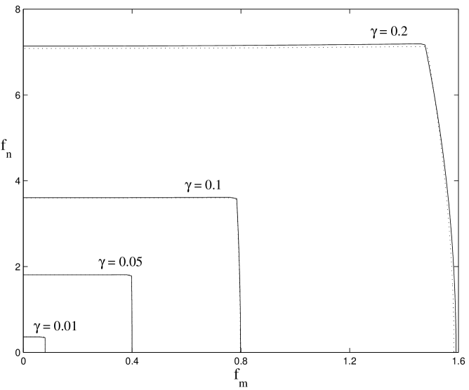
Figure 2: Linear stability boundary in $f_{m}$ - $f_{n}$ space, the parameter space of the two acceleration amplitudes in (3.1). For a given value of the damping parameter $\gamma$, the flat interface state is unstable above and to the right of the corresponding curve. Dotted lines are numerical data; solid lines correspond to the analytical expressions (3.3) and (3.3). The two are distinguishable on this graph only for $\gamma=0.2$. The other parameters are $m=4$, $n=9$, $\phi=0$ in (3.1), and $\Gamma_{0}$ = 2 in (28) - (29).

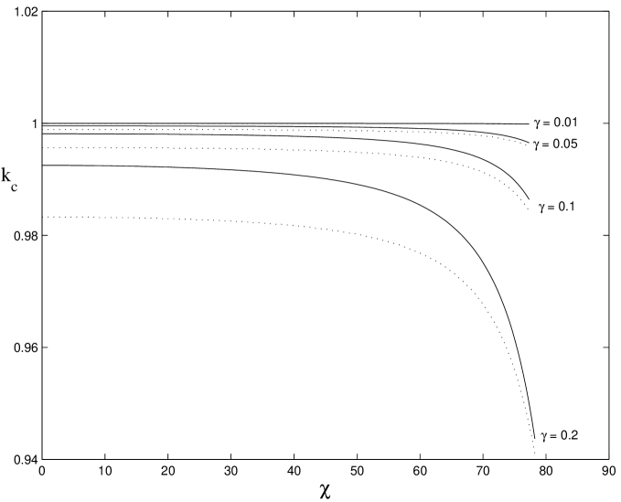
Figure 3: Critical wave number $k_{c}$ as a function of $\chi$, shown here for $\chi<\chi_{bc}$. The critical wave number decreases as the bicritical point is approached. Dotted lines are numerical data; solid lines correspond to the analytical expression (48). The parameters used are the same as those in Figure 2.

The expressions for critical acceleration and wave number were derived in section 3.3 by performing a perturbation expansion on the Zhang-Viñals equations (28) - (29) for small amplitude waves and weak damping and forcing. For arbitrary damping and forcing, the linearization of (28) - (29) is a damped Mathieu equation for each Fourier mode $p_{k}(\tau)e^{ikx}$:

$$p_{k}^{\prime\prime}+2\gamma k^{2}p_{k}^{\prime}+\left\{\gamma^{2}k^{4}+\Omega^{2}(k)\right\}p_{k}$$

$$\mbox{}=k\left\{f_{m}\cos(m\tau)+f_{n}\cos(n\tau+\phi)\right\}p_{k}.$$

where the natural frequency $\Omega(k)$ satisfies the dispersion relation (52). Thus, we may compare the results (3.3) - (48) and (3.3) - (50) with known results for the Mathieu equation with weak damping and forcing; see [28], for example. Here we focus on (3.3) and (48) which apply when the bifurcation is due to the $\cos(m\tau)$ forcing. This bifurcation corresponds to crossing through the right side of the linear stability region. Similar statements hold for crossing through the top of the linear stability region, when the bifurcation is due to the $\cos(n\tau)$ forcing, in which case (3.3) - (50) are the relevant quantities.

At leading order, the critical forcing (3.3) is proportional to the damping $\gamma$. There are two correction terms. One correction term is proportional to $\gamma^{3}$ and is independent of $f_{n}$. This term always has an overall negative sign and hence lowers $f_{m}^{c}$. The other correction term is proportional to $\gamma(f_{n})^{2}$ and is due to the second forcing component. The overall sign of this term is determined by the quantity

$$s=m^{4}+8m^{2}\Gamma_{0}-16n^{2}\Gamma_{0}-2n^{4}.$$ (75)

If $s<0$, the $\gamma(f_{n})^{2}$ term has an overall negative sign, and thus the second forcing component $\cos(n\tau)$ is destabilizing; that is to say, it pushes the bifurcation to occur at a smaller value of $f_{m}$. However, if $s>0$, the second forcing component actually stabilizes the flat fluid surface beyond those values of $f_{m}$ where it would have otherwise gone unstable.

By analyzing the expression for $s$, remembering that $\Gamma_{0}$ is restricted to the interval $0<\Gamma_{0}<m^{2}/4$, we see that there are three possible cases:

1. If $m/n<\sqrt[4]{2}$, the second frequency component is destabilizing for all values of $\Gamma_{0}$.

2. If $\sqrt[4]{2}<m/n<\sqrt{\frac{2}{3}+\frac{1}{3}\sqrt{10}}$, the second frequency component is stabilizing for $\Gamma_{0}<\Gamma_{c}=\frac{m^{4}-2n^{4}}{16n^{2}-8m^{2}}$.

3. If $m/n>\sqrt{\frac{2}{3}+\frac{1}{3}\sqrt{10}}$, the second frequency component is stabilizing for all values of $\Gamma_{0}$.

In short, the secondary forcing component is stabilizing if it is at sufficiently low frequency compared to the dominant forcing component. (However, since our results apply to weak damping and forcing, the effect of the $\gamma f_{n}^{2}$ term is quite small.)

The bicritical point $\chi_{bc}$ may be determined from (3.3) and (3.3), the expressions for critical forcing. To leading order, it is given by the simple expression

$$\chi_{bc}=\arctan{\left(\frac{nk_{n}}{m}\right)}$$ (76)

where $k_{n}$ is determined by the dispersion relation (51). Note that to leading order, $\chi_{bc}$ depends on $m$, $n$, and the capillarity number $\Gamma_{0}$, and is independent of damping and forcing. Using the bounds on $k_{n}$ that are set by the dispersion relation, we see that for a given ratio $m/n$, $\chi_{bc}$ takes on extreme values of

$$\chi_{bc}^{1}=\arctan\left(\frac{n}{m}\right)^{3}\ \mathrm{at\ \Gamma_{0}\ =\ 0}\quad\mathrm{(gravity\ waves)}$$ (77)

$$\chi_{bc}^{2}=\arctan\left(\frac{n}{m}\right)^{5/3}\ \mathrm{at\ \Gamma_{0}\ =m^{2}/4}\quad\mathrm{(capillary\ waves).}$$

For $m<n$, $\chi_{bc}^{1}$ is a maximum and $\chi_{bc}^{2}$ is a minimum; the reverse is true for $m>n$. As $\Gamma_{0}$ is changed, $\chi_{bc}$ varies smoothly and monotonically between the two extrema. Examples are shown in figure 4 for $m=4$ and various values of $n$.

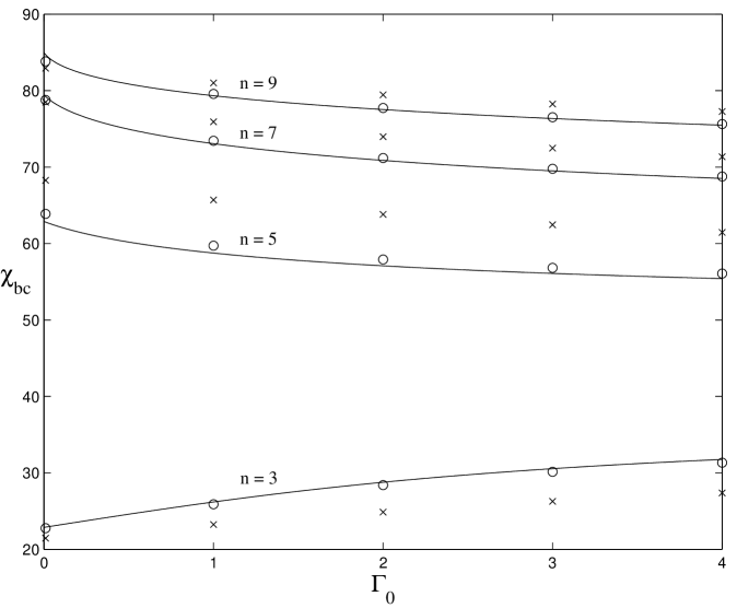
Figure 4: Bicritical point $\chi_{bc}$ (in degrees) versus capillarity parameter $\Gamma_{0}$ for $m=4$. Lines correspond to the expression in (76). Symbols correspond to a numerical computation with $\gamma=0.1$ (“o”) and $\gamma=0.4$ (“x”).

The critical wave number, to leading order, is one. This is simply the dimensionless wave number determined by the dispersion relation $\Omega^{2}(k)=(m/2)^{2}$, where $\Omega(k)$ is given by (52). There are two correction terms. One is proportional to $\gamma^{2}$ and has an overall negative sign. The other is proportional to $f_{n}^{2}$. The overall sign of this term is given by the sign of $m-n$. Therefore, the presence of the second forcing component shifts the wave number in such a way as to “repel” it from the other instability associated with the bicritical point. This effect can be seen in figure 3, which shows the critical wave number for $\chi<\chi_{bc}$.

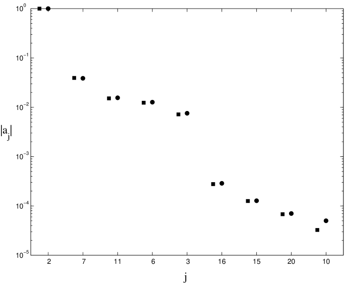
Figure 5: Magnitudes of the nine most significant fast-time frequency components in a neutrally stable Faraday mode near the bicritical point. The vertical axis (note log scale) shows the magnitude $|a_{j}|$ of the frequency component $\e^{ij\tau}$, normalized so that the largest component has magnitude one. The horizontal axis shows the Fourier index $j$. The components have been arranged in decreasing order of their magnitude. Squares correspond to data from a numerical computation. Circles follow from the perturbation analysis in section 3. The parameters used are $m=4$, $n=9$, $f_{n}=3.61$, and $\phi=0$ in (3.1), and $\gamma=0.1$ and $\Gamma_{0}$ = 2 in (28) - (29). These data are for the critical mode, with wave number $k$; the spatially resonant mode with wave number $2k$ will be dominated by a different frequency component determined by the dispersion relation (52) (e.g. $|m-n|$ if $\Gamma_{0}=\Gamma_{diff}$).

Finally, we discuss the fast-time dependence of the Faraday-unstable mode, which we write as $p(\tau)$. As demonstrated in [5], $p(\tau)$ will be harmonic or subharmonic to the period of the forcing function (3.1), namely $2\pi$. Previous work has depended on a numerically determined (truncated) Fourier series at some point in the linear or nonlinear analysis. For instance, in [5, 24, 25, 29] the time dependence of the critical mode is written as

$$p(\tau)=\sum_{j=-N}^{N}a_{j}\e^{ij\tau}$$ (78)

for the harmonic case, or

$$p(\tau)=\sum_{j=-N}^{N-1}a_{j}\e^{i(j+1/2)\tau}$$ (79)

for the subharmonic case. Then, the coefficients $a_{j}$ are determined numerically. This method assumes no a priori information about the relative importance of the frequency components kept in the expansion.

Our analysis determines the relative importance of the frequency components in $p(\tau)$ for arbitrary $m$ and $n$ in (3.1). For our perturbation expansion in section 3 we assumed that at leading order, the Faraday waves have frequency $\frac{1}{2}m$. At second order in the expansion we captured the frequency components $|n-\frac{1}{2}m|$, $n+\frac{1}{2}m$, and $\frac{3}{2}m$. At third order, we captured the components $|n-\frac{3}{2}m|$, $|2n-\frac{1}{2}m|$, $n+\frac{3}{2}m$, $2n+\frac{1}{2}m$, and $\frac{5}{2}m$.

These results are consistent with what we find numerically. Figure 5 shows the nine temporal Fourier coefficients $|a_{j}|$ that are largest, arranged in decreasing order of their magnitude. Note that even near the bicritical point, where this data was obtained, the $\frac{1}{2}m$ frequency component is at least an order of magnitude larger than any of the other components.

4.2 Nonlinear results

4.2.1 One spatial dimension

In this section we discuss the nonlinear results of section 3 for the cubic coefficient $A$ in (18). We have checked our perturbation results with numerical computations. Figure 6 shows a sample result of $A$ versus the capillarity parameter $\Gamma_{0}$ for $m/n=4/9$. The solid line corresponds to an expression which matches $A_{nonres}$ in (3.3) to $A_{diff}$ in (67) and thus is valid for all values of $\Gamma_{0}$ away from the 1:2 resonance. This expression diverges at $\Gamma_{0}=\Gamma_{1:2}=m^{2}/12$ as discussed in section 3. The dotted line corresponds to the expression $A_{1:2}$ in (61). Additionally, we have calculated the relative error in the perturbation results for $A$ as a function of the damping $\gamma$. For instance, for $m/n=4/9$ and $\chi=75^{\circ}<\chi_{bc}$, as $\gamma$ is varied from 0.05 to 0.25, the relative error in $A(\Gamma_{0}=\Gamma_{diff})$ increases from 0.001 to 0.25, and the relative error in $A(\Gamma_{0}=\Gamma_{1:2})$ increases from 0.05 to 0.43.

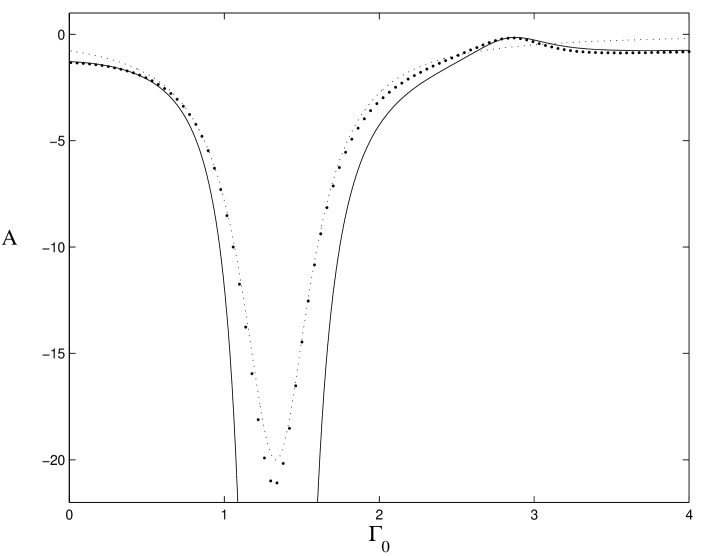
Figure 6: Cubic coefficient $A$ in (18) as a function of the capillarity parameter $\Gamma_{0}$. The dots correspond to a numerical computation. The dotted line corresponds to the expression for $A_{1:2}$ in (61). The solid line corresponds to an expression which asymptotically matches $A_{nonres}$ and $A_{diff}$ (details not given). The large dip at $\Gamma_{0}\approx\Gamma_{1:2}=4/3$ is due to the 1:2 resonance discussed in section 2.2. The small bump around $\Gamma_{0}\approx\Gamma_{diff}=17/6$, at which the one-dimensional waves have their largest amplitude, is due to the difference frequency resonance, also discussed in section 2.2. The parameters used are $m=4$, $n=9$, $\chi=75^{\circ}$ and $\phi=0$ in (3.1), and $\gamma=0.05$ in (28) - (29).

$A_{nonres}$, the value of the cubic coefficient away from the 1:2, difference, and sum frequency resonances, was computed in section 3.3 and is given by (3.3). $A_{nonres}$ is proportional to the damping parameter $\gamma$. Furthermore, $A_{nonres}$ is always negative indicating that in the nonresonant regime, the bifurcation from the flat state is always supercritical.

$A_{1:2}$, the value of the cubic coefficient near the 1:2 temporal resonance, is given by (61). This quantity was derived for $|\Gamma_{0}-\Gamma_{diff}|\simeq\mathcal{O}(\gamma)$. Thus, in the region of validity, $A_{1:2}\simeq\mathcal{O}(\gamma^{-1})$. This is significantly larger in magnitude than $A_{nonres}$, which is $\mathcal{O}(\gamma)$. Furthermore, $A_{1:2}$ is negative, again indicating a supercritical bifurcation. This large negative contribution is manifest as the large dip around $\Gamma_{0}\approx\Gamma_{1:2}=4/3$ in figure 6. $A_{1:2}$ has a global minimum at $(\Gamma_{0},A_{1:2})=(\Gamma_{1:2},-\frac{m^{2}}{16\gamma}$), so that exactly at the 1:2 resonance, the value of the coefficient $A$ is inversely proportional to the damping, as predicted by the symmetry arguments of section 2.2. Thus, near the 1:2 resonance, one-dimensional waves will decrease significantly in amplitude.

$A_{diff}$, the value of the cubic coefficient near the difference frequency resonance, is given by (67). The condition for difference frequency resonance is $\Gamma_{0}=\Gamma_{diff}$, where $\Gamma_{diff}$ is given by (63). Since $\Gamma_{0}$ is restricted to the range $[0,m^{2}/4]$, this condition can only be met for certain $m/n$ ratios. Specifically, $\Gamma_{diff}\in[0,m^{2}/4]$ only for

$$m/n\in M_{1}\cup M_{2},\quad M_{1}=[\sqrt{2}-1,2-\sqrt{2}],\quad M_{2}=[2+\sqrt{2},\infty).$$ (80)

Thus, while the 1:2 resonance was relevant for all possible forcing frequency ratios $m/n$, this is not the case for the difference frequency resonance. The difference frequency resonance results in a contribution to $A$, namely $\widehat{A}_{diff}$ given by (69), and thus $A$ has a local extremum at $\Gamma_{0}=\Gamma_{diff}$. The sign of $\widehat{A}_{diff}$ is given by the sign of $n-m$. If the secondary forcing component is at a higher frequency than the primary, i.e. if $m/n\in M_{1}$, then the difference frequency resonance results in a positive contribution to $A$. The extremum is a local maximum, and the amplitude of the supercritical waves increases as the resonance is approached. This is demonstrated by the small bump around $\Gamma_{0}\approx\Gamma_{diff}=17/6$ in figure 6. If $m/n\in M_{2}$, then the contribution is negative. The extremum is a local minimum, and the amplitude of the waves decreases. In either case, the extra contribution to $A(\Gamma_{0}=\Gamma_{diff})$ that is due to the difference frequency resonance is proportional to $(f_{n})^{2}/\gamma$ as predicted by the symmetry arguments of section 2.2, and thus is a smaller affect than the 1:2 resonance.

For the case that $m/n\in M_{1}$, when $A$ has a local maximum, it is possible for this maximum to actually cross the $A=0$ axis and become positive, thus causing the bifurcation to become subcritical. This will only happen if $f_{n}$ is sufficiently large. Writing $\widehat{A}_{diff}$ as $\widehat{a}_{diff}(f_{n})^{2}$, then the condition for a subcritical bifurcation is

$$f_{n}>\sqrt{\frac{A(\Gamma_{0}=\Gamma_{diff})}{\widehat{a}_{diff}}}.$$ (81)

Of course, condition (81) must be considered in conjunction with the condition $f_{n}<f_{n}^{c}$, which we enforced in (30). (An example of a subcritical bifurcation may be obtained with the parameters $m/n=49/100$, $\Gamma_{0}=\Gamma_{diff}=2801/12\approx 233.4$, $\gamma_{1}=0.01$ and $f_{n}=3.9<3.94\approx f_{n}^{c}$, in which case $A=0.57>0$.)

Now we turn to the results for the sum frequency resonance. $A_{sum}$ is given by (72). The condition for sum frequency resonance is $\Gamma_{0}=\Gamma_{sum}$, where $\Gamma_{sum}$ is given by (71). Similar to the difference frequency resonance case, this condition will only be met for certain $m/n$ ratios. Specifically, the sum frequency mode resonance is possible only for

$$m/n\geq\sqrt{2}+1.$$ (82)

Thus, the sum frequency resonance can only be realized when the second forcing component is at sufficiently low frequency. The sum frequency resonance results in a contribution to $A$, namely $\widehat{A}_{sum}$, which is given by (73). $A_{sum}$ has a local extremum at $\Gamma_{0}=\Gamma_{sum}$. Like the difference frequency case, the contribution to $A$ due to the sum frequency resonance is proportional to $(f_{n})^{2}/\gamma$. Unlike the difference frequency case, the $\widehat{A}_{sum}$ contribution always has a positive sign. However, this contribution is generally not significant because the algebraic prefactor in $\widehat{A}_{sum}$ is small for values of $m/n$ for which the sum frequency resonance is possible.

A partial summary of the results for 1-d resonances may be found in figure 7. This number line shows the regions of forcing frequency ratio $m/n$ in which each type of resonance is possible. The plus $(+)$ and minus $(-)$ signs indicate whether the resonance results in a positive or negative contribution to the coefficient $A$, and hence whether it makes the supercritical waves larger $(+)$ or smaller $(-)$ in amplitude.

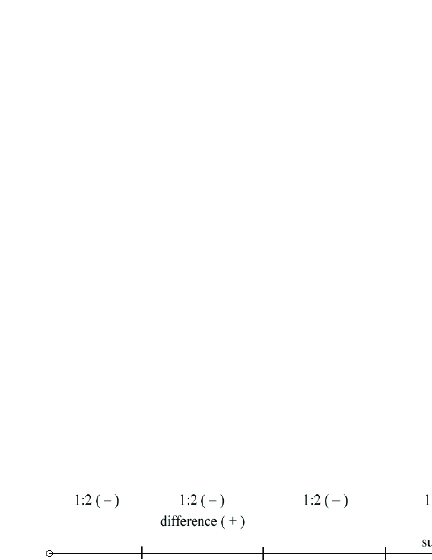
$m/n=0$         $\sqrt{2}-1$                  $2-\sqrt{2}$            $\sqrt{2}+1$                  $2+\sqrt{2}$

Figure 7: Regions of forcing frequency ratio $m/n$ in which the 1:2, difference, and sum frequency resonances are possible for one-dimensional waves. The plus $(+)$ and minus $(-)$ signs indicate whether the resonance results in a positive or negative contribution to the cubic coefficient $A$ in (18). In the case of $(-)$ the bifurcation to one-dimensional waves is necessarily supercritical. Note that only points corresponding to rational numbers on the number line are meaningful.

4.2.2 Two spatial dimensions

We now present nonlinear results for Faraday waves in two spatial dimensions. We have computed the cross-coupling coefficient $B(\theta)$ in (8) using the method in [25]. We interpret features of $B(\theta)$ in light of the resonances discussed in section 2.2. Many of these features may be understood by means of a simple argument which is valid for weak damping and forcing. We simply solve the spatial resonance condition (2) or (4) for $\theta_{1:2}$, $\theta_{sum}$ or $\theta_{diff}$, which are the angles at which the 1:2, sum frequency, and difference frequency resonances occur. To do this, we must set $|\mathbf{k}_{3}|=k(\Omega)$ where $k(\Omega)$ is the inverse of the dispersion relation (52) and $\Omega=m$, $m+n$ or $|m-n|$ depending on the resonance under consideration. A number of results immediately follow:

• The 1:2 resonance is possible only for $\Gamma_{0}\geq m^{2}/12=\Gamma_{1:2}$.

• The difference frequency resonance is possible only for

  $$m-\frac{1}{2}\sqrt{2m^{2}+24\Gamma_{0}}\leq n\leq m+\frac{1}{2}\sqrt{2m^{2}+24\Gamma_{0}}.$$ (83)

• The sum frequency resonance is possible only for $n\leq-m+\frac{1}{2}\sqrt{2m^{2}+24\Gamma_{0}}$.

From these statements, we also see that

• The ranges of $\theta_{1:2}$, $\theta_{sum}$ and $\theta_{diff}$ are restricted.

• There are some forcing frequency ratios $m/n$ for which the sum and difference frequency resonances are not possible for any value $\Gamma_{0}$.

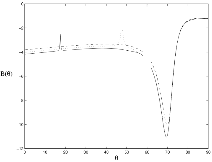
Figure 8: Cross-coupling coefficient $B(\theta)$ in (8). The solid line corresponds to $m/n=8/9$ in (3.1); the dotted and dashed lines correspond to $m/n=8/11$ and $8/21$ respectively. For each curve, the parameter $\chi$ is chosen to obtain a harmonic instability near the bicritical point. The other parameters are $\phi=0$ in (3.1), and $\Gamma_{0}=14$ and $\gamma=0.1$ in (28) - (29). The large dip at $\theta=\theta_{1:2}\approx 70^{\circ}$ is due to the 1:2 temporal resonance discussed in section 2.2 and is independent of the second forcing component. The small spike is due to the difference frequency resonance discussed in section 2.2. We have removed from this plot the region near $\theta=60^{\circ}$ where $B(\theta)$ necessarily diverges; a calculation for the hexagonal lattice is required here.

An example is given in figure 8, which shows the cross-coupling coefficient $B(\theta)$ computed for forcing frequency ratios $m/n=8/9$, $8/11$ and $8/21$ for fixed fluid parameters; $\chi$ is chosen in each case to obtain a harmonic instability near the bicritical point. The large dip at $\theta=\theta_{1:2}\approx 70^{\circ}$ is consequence of the 1:2 resonance. At this angle, which is predicted by the weak damping argument given above, there is a resonant triad comprised of two Faraday-unstable modes with dominant frequency $m/2$ and the weakly damped mode oscillating primarily with the harmonic frequency $m$. As expected from the analysis of section 2.2, near this angle, the weakly damped mode contributes to $B(\theta)$, which here is manifest as the large dip. This phenomenon is similar to the 1:2 resonance in one spatial dimension, which resulted in a large dip in the cubic self-interaction coefficient A in (18). It follows from the weak damping argument that $\theta_{1:2}$ will depend on $m$ and $\Gamma_{0}$ but will be largely independent of the parameters $n$, $f_{n}$, and $\gamma$. The independence with respect to $n$ is evident in figure 8, in which the dip occurs at the same angle for $m/n=8/9$, $8/11$, and $8/21$.

For all numerical calculations that we performed, the 1:2 resonance resulted in a large negative contribution to the cross-coupling coefficient $B(\theta)$. As discussed in section 2.1, this type of contribution is destabilizing for superlattice patterns with characteristic angles $\theta_{h}$near $\theta_{1:2}$. Our numerical results (not shown) indicate that the magnitude of the dip caused by the 1:2 resonance follows the scaling law that we deduced from symmetry considerations in section 2.2, and that we derived for one-dimensional waves: namely, that the contribution from the weakly damped mode scales like $1/\gamma$.

The sum frequency resonance angle $\theta_{sum}$ may also be predicted by the weak damping argument. However, unlike the 1:2 resonance described above and the difference frequency resonance described below, the sum frequency resonance for two dimensional waves is quite difficult to detect numerically for typical values of $m/n$ and for small $\gamma$. This is consistent with the result for one spatial dimension, and consistent with the fact that the mode oscillating at the sum frequency has a larger wave number and thus is more strongly damped.

Finally, we turn to results for the difference frequency resonance. The effect of the difference frequency resonance may be seen in figure 8, and is manifest as a spike in the plot of $B(\theta)$. Let us first concentrate on the solid curve in figure 8, which corresponds to a forcing frequency ratio of $m/n=8/9$. For this case, at $\theta=\theta_{diff}\approx 17^{\circ}$ there is a resonant triad composed of two modes with dominant frequency $m/2$ and the weakly damped mode oscillating with dominant frequency $|n-m|$. As expected from the analysis of section 2.2, near this angle, the weakly damped mode contributes to $B(\theta)$, which causes the spike. This phenomenon is similar to the difference frequency resonance in one spatial dimension, which resulted in a contribution to the cubic self-interaction coefficient $A$.

As with the case of 1:2 resonance, the simple argument we have used to predict the resonance angle $\theta_{diff}$ relies only on the dispersion relation (52) and on the trigonometric relations (3) and (5). By examining these two expressions, we expect that $\theta_{diff}$ will depend on $m$, $n$, and $\Gamma_{0}$ but will be largely independent of the parameters $f_{n}$ and $\gamma$. The dependence on the second forcing frequency $n$ is evident in figure 8, in which shifting from $n=9$ to $n=11$ causes the spike to shift from $\theta_{diff}\approx 17^{\circ}$ to $\theta_{diff}\approx 47^{\circ}$.

Figure 9 shows the angle of spatial resonance $\theta_{diff}$ versus the capillarity parameter $\Gamma_{0}$ for the forcing frequency ratios $m/n=8/9$ and $8/11$ and for various values of $\gamma$. The solid lines represent the prediction of $\theta_{diff}$ based on the weak-damping argument, while the points represent data from a full numerical computation of $B(\theta)$.

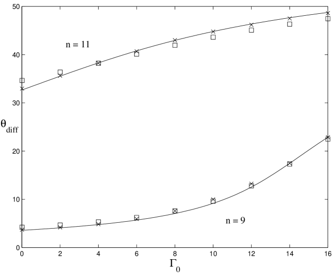
Figure 9: Angle of spatial resonance $\theta_{diff}$ versus capillarity number $\Gamma_{0}$. Lines correspond to a prediction of $\theta_{diff}$ based on the dispersion relation (52) and on the trigonometric relation (5). Symbols correspond to a numerical calculation of $\theta_{diff}$: $\gamma=0.2$ (“x”), $\gamma=0.8$ (“$\square$”). The other parameters are $m=8$, $\chi=50^{\circ}$ and $\phi=0$ in (3.1).

Another result that follows from the weak damping arguments is that if the second forcing frequency $n$ is sufficiently different from $m$, the difference frequency resonance will not be possible for any value of $\Gamma_{0}$. This phenomenon is demonstrated in figure 8. The forcing frequency ratio $m/n=8/21$ violates the condition (83) for all allowed $\Gamma_{0}$, and the corresponding $B(\theta)$ curve (dashed line) displays only the 1:2 resonance effect.

Now we discuss the magnitude and direction of the difference frequency mode resonance effect. In contrast to the 1:2 resonance, we find that the difference frequency resonance may result in a spike or a dip. Limited numerical results for the sign of the resonance effect agree with the result for one spatial dimension discussed in section 4.2.1. In particular, we have performed computations at $\gamma=0.1$ for the forcing frequency ratios $m/n=8/7$, $8/9$, $8/11$, $10/7$, $10/9$ and $10/11$, each for values of $\Gamma_{0}$ ranging between $0$ and $\Gamma_{max}=m^{2}/4$. In all cases, we observe that if $n<m$ then the difference frequency resonance results in a dip at $\theta=\theta_{diff}$; if $n>m$, it results in a spike. An example of the former case is shown in figure 10, which corresponds to a forcing frequency ratio of $m/n=8/7$. The resonant wave number $k_{d}$ and the angle of spatial resonance $\theta_{diff}$ are (approximately) the same as for the case $m/n=8/9$ shown in figure 8; however, the difference frequency mode resonance now results in a very small dip rather than a spike, as before.

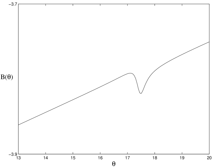
Figure 10: Cross-coupling coefficient $B(\theta)$ for forcing frequency ratio $m/n=8/7$ in (3.1). The difference frequency resonance results in a small dip around $\theta=\theta_{diff}\approx 17^{\circ}$. This is in contrast to the case $m/n=8/9$, which produces a spike at the same angle. The other parameters are $\chi\approx 37^{\circ}$ and $\phi=0$ in (3.1), and $\gamma=0.1$ and $\Gamma_{0}=14$ in (28) - (29).

As in the one-dimensional case, the magnitude of the difference frequency resonance effect follows the scaling law that we deduced from symmetry considerations in section 2.2, namely that the contribution from the weakly damped mode scales like $(f_{n})^{2}/\gamma$. This scaling may be seen in figure 11. We compute the magnitude of the effect by finding $B(\theta_{diff})-B_{f_{n}=0}(\theta_{diff})$, where $B_{f_{n}=0}(\theta_{diff})$ is the value of the cross-coupling coefficient at the resonant angle computed without the second forcing component. We plot the size of the spike versus $(f_{n})^{2}/\gamma$.

Figure 11: $B(\theta_{diff})-B_{f_{n}=0}(\theta_{diff})$, the magnitude of the difference frequency spike, versus $(f_{n})^{2}/\gamma$. The damping parameter $\gamma$ is varied between 0.01 and 0.1, and the strength of the second forcing frequency $f_{n}$ is varied between 0 (which corresponds to single frequency forcing) and $f_{n}^{c}$. Best-fit lines are also shown. The other parameters are $m=8$ and $\phi=0$ in (3.1), and $\Gamma_{0}=14$ in (28) - (29).

As discussed in section 2.1, a spike occurring at spatial angle $\theta=\theta_{diff}$ will help stabilize SL-I patterns with characteristic angles $\theta_{h}$ near $\theta_{diff}$. To demonstrate this effect, we consider an example for $m/n=8/11$ forcing, with $\gamma=0.2$, and $\Gamma_{0}=13$ and focus on the case of a harmonic instability. These dimensionless parameters can be realized, for instance, by a fluid with surface tension $\Gamma=4.2\ \mathrm{dyn/cm}$, density $\rho=1.0\ \mathrm{g/cm^{3}}$, and kinematic viscosity $\nu=0.01\ \mathrm{cm^{2}/s}$ being forced with base frequency $\omega/(2\pi)=16.2\ \mathrm{Hz}$. (The fluid properties here are similar to those of water, but with lower surface tension. This situation might be achieved by the use of a surfactant).

When $\chi=60.5^{\circ}$, there is a spike in $B(\theta)$ at $\theta_{diff}=46.9^{\circ}$, which is close to the value of $47.0^{\circ}$ that is predicted by the weak-damping argument. We have performed a limited bifurcation analysis similar to that in [25]. The stability of SL-I patterns is computed with respect to simple rolls, simple hexagons, and various rhombic patterns. An SL-I pattern with lattice angle $\theta_{h}\approx 47^{\circ}$ is stable for a small range of $f$ above, but bounded away from, onset. A higher order calculation is necessary to determine whether it is the superhexagon or supertriangle variety of SL-I pattern that is stabilized (these two different types of SL-I patterns have different phases associated with the complex amplitude). When $\chi=0^{\circ}$ (i.e. when there is only single frequency forcing) the spike in $B(\theta)$ due to the difference frequency disappears and the SL-I patterns with $\theta_{h}\approx 47^{\circ}$ are unstable. Superhexagon and supertriangle solutions with $\theta_{h}\approx 47^{\circ}$ are shown in figure 12.

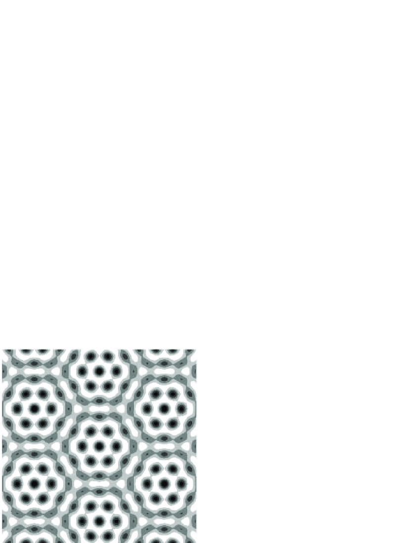
Figure 12: Superhexagon (left) and supertriangle (right) patterns with characteristic angle $\theta_{h}\approx 47^{\circ}$. For $m/n=8/11$ forcing with $\gamma=0.2$ and $\Gamma_{0}=13$, both patterns are unstable for $\chi=0^{\circ}$. For $\chi=60.5^{\circ}<\chi_{bc}$, one of these patterns is stabilized by the difference frequency resonance effect; a higher order calculation is needed to determine which one. The patterns shown were created by an appropriate superposition of the twelve critical Fourier modes [18].

5 Conclusions

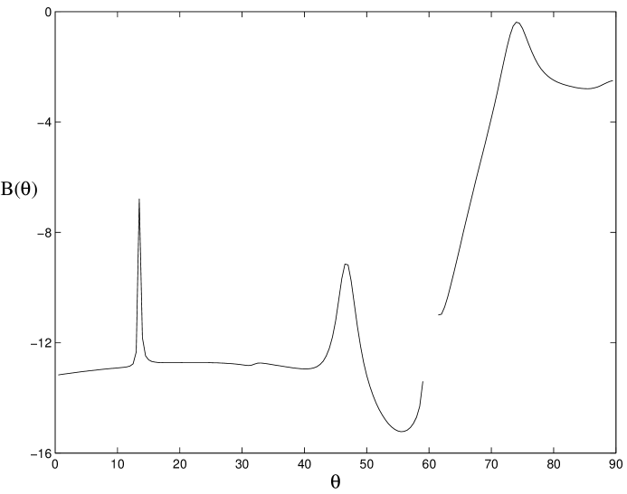
Figure 13: Cross-coupling coefficient $B(\theta)$ in (8) computed for the case of a four-frequency forcing function analogous to (3.1), with frequency components $(m,n,p,q)=(8,9,11,13)$. For this calculation, the $m=8$ forcing component dominates, but we are near a “quad-critical” point so that the other three frequency components are strong. The three spikes at $\theta=13^{\circ},\ 47^{\circ},\ 73^{\circ}$ are due to resonances with the weakly damped modes oscillating with the difference frequencies $n-m$, $p-m$ and $q-m$. The other parameters used are $\Gamma_{0}=12.4$ and $\gamma=0.25$ in (28) - (29). The stability of the SL-I patterns with $\theta_{h}\approx 13^{\circ}$ is enhanced by the additional spikes at $\theta\approx 60^{\circ}\pm\theta_{h}$; see [25] for a detailed discussion of how these two additional symmetry-related angles are relevant.

In this paper we have examined the role that weakly damped modes play in the pattern selection process for Faraday waves forced with frequency components $m\omega$ and $n\omega$. Our symmetry arguments predict that the modes oscillating primarily with the harmonic frequency $m\omega$, the difference frequency $|n-m|\omega$, and the sum frequency $(n+m)\omega$ will be the most important in terms of their contribution to the cubic coefficients $A$ and $B(\theta)$ in the standing wave equations (8). The symmetry considerations also provided scaling laws for the magnitude of these resonance effects.

Starting with the Zhang-Viñals Faraday wave equations, we performed a weakly nonlinear analysis for weak damping and forcing in order to calculate expressions for the self-interaction coefficient $A$. We obtained expressions for the critical forcing acceleration and wave number, and analyzed them to elucidate the role played by the secondary forcing component. We also were able to identify the most important frequency components in the unstable eigenmode in terms of the integers $m$ and $n$. We then analyzed the expression for the cubic coefficient $A$, and determined the sign and scaling of contributions due to the various resonance effects.

We then used the Zhang-Viñals equations to numerically calculate the cross-coupling coefficient $B(\theta)$ according to the method in [25]. The predictions of the symmetry arguments were manifest. The results for $B(\theta)$ are of particular interest since this coefficient is crucial in determining the stability of SL-I patterns like those observed in [2]. We made use of a weak-damping argument relying only on the dispersion relation to successfully predict the resonant angle. While our symmetry arguments predict the scaling of the resonance effects and our weak-damping argument predicts the angle, neither argument predicts the sign of the contribution to $B(\theta)$. Our numerical calculation revealed that the 1:2 resonance results in a dip, and thus is destabilizing for SL-I patterns. However, the difference frequency resonance in some cases results in a spike, which can help stabilize SL-I patterns with characteristic angles near the resonant angle $\theta_{diff}$. This was demonstrated by means of a simple bifurcation example.

We may now speculate on the role of the bicritical point in stabilizing SL-I patterns. It is been observed that SL-I patterns occur in experiments only for parameters near the bicritical point. It is tempting to believe, then, that the weakly damped mode associated with the secondary forcing component is somehow responsible for the pattern. Here we have shown that this interpretation is not necessarily the correct one. Proximity to the bicritical point (i.e. making $f_{n}$ as large as possible before switching over to the other instability) maximizes the strength of the difference frequency mode. As we have seen, this mode can help stabilize the SL-I pattern.

It will be interesting to consider Faraday waves forced with more than two frequency components. In this case, more difference frequency mode resonances will be possible. As demonstrated in figure 13, if the parameters are chosen properly, multiple spikes in the cross-coupling coefficient $B(\theta)$ might conspire to further enhance the stability of a particular superlattice pattern.

Appendix A Appendix A

We now give the expressions for the coefficients in the travelling wave equations (36) - (3.3), (59) and (66) which we computed in section 3.

$$\eta_{1} = -\frac{f_{m}^{1}}{2m}$$ (84)

$$\nu_{2} = \frac{k_{2}(8\Gamma_{0}+m^{2})}{4m}+\frac{3(f_{m}^{1})^{2}}{8m^{3}}+\frac{(f_{n}^{1})^{2}}{2m(n^{2}-m^{2})}$$ (85)

$$c_{1} = \frac{2m^{4}-15m^{2}\Gamma_{0}+36\Gamma_{0}^{2}}{2m(m^{2}-12\Gamma_{0})}$$ (86)

$$c_{2} = -\frac{2m^{4}+15m^{2}\Gamma_{0}+36\Gamma_{0}^{2}}{m(m^{2}+12\Gamma_{0})}$$ (87)

$$\gamma_{3} = 2\gamma_{1}k_{2}$$ (88)

$$\eta_{3} = -\frac{9(f_{m}^{1})^{3}}{32m^{5}}+\frac{f_{m}^{1}(f_{n}^{1})^{2}(m^{4}-m^{2}n^{2}-n^{4})}{2n^{2}m^{3}(n^{2}-m^{2})^{2}}$$

$$\mbox{}-\frac{f_{m}^{1}k_{2}(8\Gamma_{0}+3m^{2})}{4m^{3}}-\frac{f_{m}^{3}}{2m}$$

$$c_{3} = -\frac{\gamma_{1}(7m^{4}-48m^{2}\Gamma_{0}+144\Gamma_{0}^{2})}{(m^{2}-12\Gamma_{0})^{2}}$$ (90)

$$c_{4} = \frac{6\gamma_{1}(m^{2}+4\Gamma_{0})}{m^{2}+12\Gamma_{0}}$$ (91)

$$c_{5} = \frac{3f_{m}^{1}(4m^{8}-47m^{6}\Gamma_{0}+516m^{4}\Gamma_{0}^{2}+2160m^{2}\Gamma_{0}^{3}+8640\Gamma_{0}^{4})}{4m^{3}(m^{2}+12\Gamma_{0})(m^{2}-12\Gamma_{0})^{2}}$$ (92)

$$c_{6} = \frac{3f_{m}^{1}(4m^{6}-63m^{4}\Gamma_{0}-240m^{2}\Gamma_{0}^{2}-720\Gamma_{0}^{3})}{8m^{3}(m^{2}+12\Gamma_{0})(m^{2}-12\Gamma_{0})}$$ (93)

$$c_{7} = -\frac{f_{m}^{1}(4m^{6}-39m^{4}\Gamma_{0}+144m^{2}\Gamma_{0}^{2}+432\Gamma_{0}^{3})}{8m^{3}(m^{2}+12\Gamma_{0})(m^{2}-12\Gamma_{0})}$$ (94)

$$e_{1} = \frac{m}{2}$$ (95)

$$\gamma_{4} = 4\gamma_{1}$$ (96)

$$\nu_{4} = \frac{3\widehat{\Gamma}_{1:2}}{m}$$ (97)

$$e_{2} = \frac{m}{4}$$ (98)

$$\widetilde{\nu}_{4} = -\frac{3\widehat{\Gamma}_{diff}}{n-m}$$ (99)

$$r_{1} = \frac{\e^{i\phi}f_{n}^{1}(2n^{2}-4nm+m^{2})}{2n(m-n)(2m-n)}$$ (100)

$$c_{8} = \frac{48n^{6}-72n^{3}m^{3}+204m^{2}n^{4}-176n^{5}m}{4nm(m-n)(m^{2}-10nm+6n^{2})}$$

$$\mbox{}-\frac{m^{6}+8nm^{5}-8m^{4}n^{2}}{4nm(m-n)(m^{2}-10nm+6n^{2})}$$

$$c_{9} = -\frac{48n^{6}-2200n^{3}m^{3}+1324m^{2}n^{4}-400n^{5}m}{4m(6n^{2}-14nm+5m^{2})(2m^{2}-3nm+n^{2})}$$

$$\mbox{}-\frac{143m^{6}-824nm^{5}+1912m^{4}n^{2}}{4m(6n^{2}-14nm+5m^{2})(2m^{2}-3nm+n^{2})}$$

$$\nu_{5} = \frac{9\widehat{\Gamma}_{diff}^{2}}{2(m-n)^{3}}-\frac{(f_{m}^{1})^{2}}{(3m-2n)(m-2n)(m-n)}$$

$$\mbox{}-\frac{(f_{n}^{1})^{2}}{(2m-n)(2m-3n)(m-n)}+\frac{k_{2}(7m^{2}-22nm+11n^{2})}{6(m-n)}$$

$$r_{2} = \frac{\e^{-i\phi}mf_{n}^{1}(m^{2}-4nm+2n^{2})}{4n(m-n)^{2}(2m-n)}$$ (104)

$$c_{10} = \frac{c_{8}m}{m-n}$$ (105)

$$c_{11} = \frac{c_{9}m}{m-n}$$ (106)

$$c_{12} = \frac{2(2n^{4}-8n^{3}m+9m^{2}n^{2}-2m^{3}n+m^{4})}{(n-m)(3n^{2}-6nm+m^{2})}$$ (107)

$$c_{13} = \frac{4(119m^{2}n^{2}-62m^{3}n+11m^{4}+22n^{4}-88n^{3}m)}{(n-m)(5n^{2}-10nm+3m^{2})}$$ (108)

References

- [1] W. Zhang and J. Viñals. Pattern formation in weakly damped parametric surface waves. J. Fluid Mech., 336:301–330, Apr. 1997.
- [2] A. Kudrolli, B. Pier, and J.P. Gollub. Superlattice patterns in surface waves. Physica D, 123(1–4):99–111, Nov. 1998.
- [3] M. Faraday. On the forms and states of fluids on vibrating elastic surfaces. Phil. Trans. R. Soc. Lond., 121:319–340, 1831.
- [4] H.W. Müller, R. Friedrich, and D. Papathanassiou. Theoretical and experimental investigations of the Faraday instability. In F. Busse and S.C. Müller, editors, Evolution of Spontaneous Structures in Dissipative Continuous Systems, Lecture Notes in Physics, pages 231–265. Springer, Jul. 1998.
- [5] T. Besson, W.S. Edwards, and L. Tuckerman. Two-frequency parametric excitation of surface waves. Phys. Rev. E, 54(1):507–513, Jul. 1996.
- [6] H.W. Müller. Periodic triangular patterns in the Faraday experiment. Phys. Rev. Lett., 71(20):3287–3290, Nov. 1993.
- [7] W.S. Edwards and S. Fauve. Patterns and quasi-patterns in the Faraday experiment. J. Fluid Mech., 278:123–148, Nov. 1994.
- [8] H. Arbell and J. Fineberg. Spatial and temporal dynamics of two interacting modes in parametrically driven surface waves. Phys. Rev. Lett., 81(20):4384–4387, Nov. 1998.
- [9] H. Arbell and J. Fineberg. Two-mode rhomboidal states in driven surface waves. Phys. Rev. Lett., 84(4):654–657, Jan. 2000.
- [10] H. Arbell and J. Fineberg. Pattern formation in two-frequency forced parametric waves. Preprint, 2001.
- [11] E. Pampaloni, S. Residori, S. Soria, and F.T. Arecchi. Phase locking in nonlinear optical patterns. Phys. Rev. Lett., 78(6):1042–1045, Feb. 1997.
- [12] J.L. Rogers, M.F. Schatz, J.L. Bougie, and J.B. Swift. Rayleigh–Bénard convection in a vertically oscillated fluid layer. Phys. Rev. Lett., 84(1):87–90, Jan. 2000.
- [13] J.L. Rogers, M.F. Schatz, O. Brausch, and W. Pesch. Superlattice patterns in vertically oscillated Rayleigh-Bénard convection. Phys. Rev. Lett., 85(20):4281–4284, Nov. 2000.
- [14] C. Wagner, H.W. Müller, and K. Knorr. Pattern formation at the bicritical point of the Faraday instability. Preprint, 2001.
- [15] H.S. Wi, K. Kim, and H.K. Pak. Pattern selection on granular layers under multiple frequency forcing. J. Kor. Phys. Soc., 38(5):573–576, May 2001.
- [16] D.P. Tse, A.M. Rucklidge, R.B. Hoyle, and M. Silber. Spatial period-multiplying instabilities of hexagonal Faraday waves. Physica D, 146(1–4):367–387, Nov. 2000.
- [17] A. Rucklidge, M. Silber, and J. Fineberg. Secondary instabilities of hexagons: A bifurcation analysis of experimentally observed Faraday wave patterns. In J. Buescu, S. Castro, A.P. Dias, and I. Labouriau, editors, Bifurcations, Symmetry and Patterns, Basel, 2002. Birkhauser.
- [18] M. Silber and M.R.E. Proctor. Nonlinear competition between small and large hexagonal patterns. Phys. Rev. Lett, 81(12):2450–2453, Sep. 1998.
- [19] D. Binks and W. van de Water. Nonlinear pattern formation of Faraday waves. Phys. Rev. Lett., 78(21):4043–4046, May 1997.
- [20] D. Binks, M.T. Westra, and W. van de Water. Effect of depth on the pattern formation of Faraday waves. Phys. Rev. Lett., 79(25):5010–5013, Dec. 1997.
- [21] W. Zhang and J. Viñals. Pattern formation in weakly damped parametric surface waves driven by two frequency components. J. Fluid Mech., 341:225–244, Jun. 1997.
- [22] R. Lifshitz and D.M. Petrich. Theoretical model for Faraday waves with multiple-frequency forcing. Phys. Rev. Lett., 79(7):1261–1264, Aug. 1997.
- [23] P. Chen and J. Viñals. Amplitude equation and pattern selection in Faraday waves. Phys. Rev. E, 60(1):559–570, Jul. 1999.
- [24] M. Silber and A.C. Skeldon. Parametrically excited surface waves: Two-frequency forcing, normal form symmetries, and pattern selection. Phys. Rev. E, 59(5):5446–5456, May 1999.
- [25] M. Silber, C.M. Topaz, and A.C. Skeldon. Two-frequency forced Faraday waves: Weakly damped modes and pattern selection. Physica D, 143(1–4):205–225, Sep. 2000.
- [26] J. Porter and M. Silber. Resonant triad dynamics in weakly damped Faraday waves with two-frequency forcing. In prep., 2001.
- [27] J. Porter. Personal communication; see also [26].
- [28] D.W. Jordan and P. Smith. Nonlinear Ordinary Differential Equations. Oxford Applied and Engineering Mathematics. Oxford University Press, Oxford, 1999.
- [29] K. Kumar and L.S. Tuckerman. Parametric instability of the interface between two fluids. J. Fluid Mech., 279:49–68, Nov. 1994.